Flood-related extreme precipitation in southwestern Germany: development of a two-dimensional stochastic precipitation model - HESS
←
→
Page content transcription
If your browser does not render page correctly, please read the page content below
Hydrol. Earth Syst. Sci., 23, 1083–1102, 2019
https://doi.org/10.5194/hess-23-1083-2019
© Author(s) 2019. This work is distributed under
the Creative Commons Attribution 4.0 License.

Flood-related extreme precipitation in southwestern Germany:
development of a two-dimensional stochastic precipitation model
Florian Ehmele1 and Michael Kunz1,2
1 Instituteof Meteorology and Climate Research, Karlsruhe Institute of Technology (KIT),
Hermann-von-Helmholtz-Platz 1, 76344 Eggenstein-Leopoldshafen, Germany
2 Center for Disaster Management and Risk Reduction Technology (CEDIM), KIT – Karlsruhe, Karlsruhe, Germany

Correspondence: Florian Ehmele (florian.ehmele@kit.edu)

Received: 22 March 2018 – Discussion started: 16 April 2018
Revised: 8 February 2019 – Accepted: 11 February 2019 – Published: 25 February 2019

Abstract. Various fields of application, such as risk assess-     estimated return periods of more than 200 years (Schröter
ments of the insurance industry or the design of flood protec-    et al., 2015) resulted in losses of more than EUR 22 billion
tion systems, require reliable precipitation statistics in high   (inflation adjusted to 2017; MunichRe, 2017). In addition to
spatial resolution, including estimates for events with high      these rare extreme events, less-severe floods with shorter re-
return periods. Observations from point stations, however,        turn periods, such as in 2005, 2006, 2010, and 2011 (Uh-
lack of spatial representativeness, especially over complex       lemann et al., 2010; Kienzler et al., 2015), also contribute
terrain. Current numerical weather models are not capable         significantly to the large average annual losses from floods
of running simulations over thousands of years. This pa-          of EUR 1.1 billion in Germany in the last 30 years (Mu-
per presents a new method for the stochastic simulation of        nichRe, 2017). Flood risk estimation, for example, for in-
widespread precipitation based on a linear theory describ-        surance purposes or for the design of appropriate flood pro-
ing orographic precipitation and additional functions that        tection systems, requires comprehensive statistical analyses
consider synoptically driven rainfall and embedded convec-        of both runoff and rainfall. Traditionally, extremes associ-
tion in a simplified way. The model is initialized by various     ated with the latter have been estimated at point stations from
statistical distribution functions describing prevailing atmo-    the intensity–duration–frequency (IDF), with extreme value
spheric conditions such as wind vector, moisture content, or      statistics being applied (Koutsoyiannis et al., 1998). This
stability, estimated from radiosonde observations for a lim-      method, however, implies two major difficulties: (i) the low
ited sample of observed heavy rainfall events. The model is       density of point observations and their limited representative-
applied for the stochastic simulation of heavy rainfall over      ness, in particular over complex terrain, and (ii) the limited
the complex terrain of southwestern Germany. It is shown          observation period with the consequence that not all possible
that the model provides reliable precipitation fields despite     extreme configurations enter the samples.
its simplicity. The differences between observed and simu-           To account for the former issue, geostatistical interpolation
lated rainfall statistics are small, being of the order of only   routines, such as kriging (Goovaerts, 2000), or techniques
 ± 10 % for return periods of up to 1000 years.                   relating precipitation to orographic or atmospheric charac-
                                                                  teristics (e.g., Basist et al., 1994; Drogue et al., 2002) have
                                                                  been applied. Recently, Marra et al. (2017) showed that IDFs
                                                                  can be reliably estimated from remote sensing data, such as
1   Introduction                                                  weather radars, with high spatial coverage. However, the con-
                                                                  version from radar reflectivity to rain intensity leads to high
Severe pluvial flood events resulting from persistent rainfall    uncertainty, mainly because of the unknown drop size distri-
over large areas have the potential to cause high economic        bution in combination with the radar reflectivity being pro-
losses of several billion euros (EUR) in central Europe. In       portional to the drop diameter in the sixth power. Compar-
Germany, the two extreme floods of 2002 and 2013 with

Published by Copernicus Publications on behalf of the European Geosciences Union.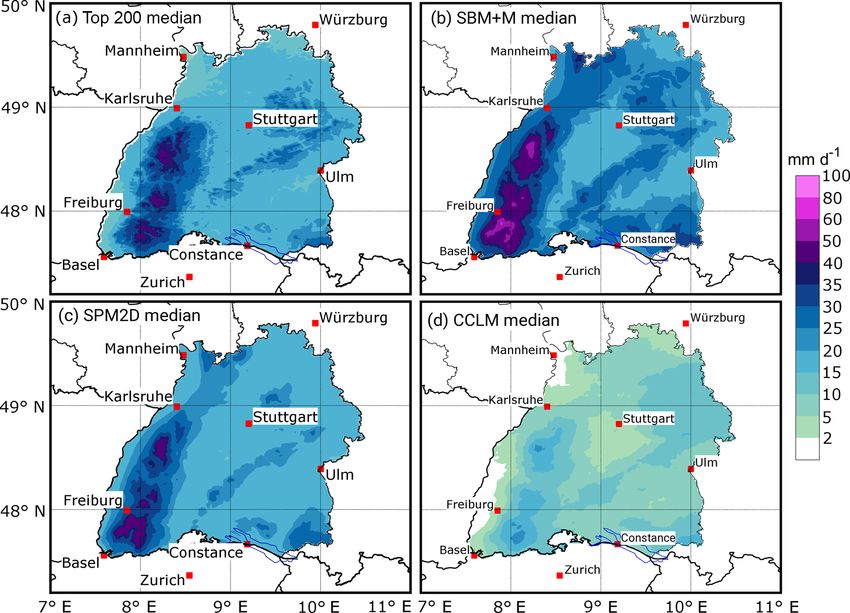
1084                                                                   F. Ehmele and M. Kunz: Stochastic precipitation model

ing IDFs obtained from radar data with point observations          over the whole investigation area and for the time period of
on a local scale, Peleg et al. (2018) found that the spatial       the soundings, usually 12 h. For the stochastic simulations,
IDFs tend to underestimate rainfall intensity for short return     these input parameters are varied randomly based on appro-
periods and that the natural variability of extreme rainfall in-   priate PDFs derived from a representative sample of histor-
creases the uncertainties of the IDFs for longer return periods    ical heavy rainfall events. Because precipitation regimes in
and larger areas.                                                  summer and winter vary significantly, we seasonally differ-
   To account for the limited observation period, several stud-    entiate our analyses. The SPM2D is one component of a
ies have employed stochastic weather generators to simu-           novel risk assessment method to quantify the probable max-
late precipitation events at single grid points (e.g., Richard-    imum loss for a 200-year event (PML200) by considering
son, 1981; Furrer and Katz, 2007; Neykov et al., 2014).            simultaneous flooding along the main river networks. This
A recent study by Cross et al. (2018), for example, intro-         paper, however, discusses only on the precipitation or hazard
duced a censored rainfall modeling approach designed to            component.
reduce the underestimation of extremes. In addition, some             The paper is structured as follows. Sect. 2 introduces the
two-dimensional stochastic weather generators are currently        basic concept of the SPM2D. Section 3 briefly describes the
available. The Space–Time Realizations of Areal Precipita-         data sets used in this study. Section 4 presents the results of
tion model (STREAP) by Paschalis et al. (2013), for instance,      the calibration based on a set of 200 representative histor-
uses probability density functions (PDFs) for sequences of         ical heavy rainfall events and examines sensitivities of the
wet and dry periods to stochastically create storms. In be-        model depending on varying ambient conditions. Section 5
tween the single storm events, the spatial distribution of pre-    shows some characteristics of the selected events. Results of
cipitation is simulated using auto- and cross-correlations be-     the stochastic simulations are discussed in Sect. 6, and Sect. 7
tween the single grid cells of the investigation area. Based       lists some conclusions. Further information is given in a short
on that, Peleg et al. (2017) extended the STREAP model             Appendix and Supplement.
to a semi-physical level by implementing physical correla-
tions between different climate variables like cloud cover
and precipitation. The spatial distribution, however, is still     2     Stochastic precipitation model
calculated in a statistical way. Other pure statistically based
                                                                   The SPM2D model is designed for the simulation of
weather generators have recently been presented by Benoit
                                                                   widespread, pluvial precipitation over complex terrain such
et al. (2018) or Singer et al. (2018). Albeit considering the
                                                                   as low mountain ranges, a typical feature of European to-
long-term variability of precipitation, which leads to more
                                                                   pography. The investigation area for this study is the federal
reliable estimates for extremes, these approaches still have a
                                                                   state of Baden-Württemberg (BW) in southwestern Germany
limited physically justified spatial representativeness.
                                                                   (Fig. 1). The terrain exhibits a certain degree of complexity,
   Furthermore, robust estimates of precipitation extremes
                                                                   with the broad Rhine Valley with elevations of 100–200 m
with high return periods, for example, for an event happen-
                                                                   bounded by the Vosges mountains (France) to the west and
ing once in 200 years, require a large sample size of sev-
                                                                   the Black Forest mountains to the east. The highest peak is
eral thousands of events. Current numerical weather predic-
                                                                   the Feldberg, with a maximum elevation of 1493 m, in south-
tion (NWP) models, though having a high spatial resolution
                                                                   ern Black Forest. To the northeast, the topography is more
of several kilometers, are not able to simulate thousands of
                                                                   flat with some rolling terrain. Annual precipitation varies be-
events due to their complexity and the resulting high com-
                                                                   tween 600 mm (southern Rhine Valley) and approximately
puting costs.
                                                                   2000 mm (southern Black Forest).
   In this study we present a semi-physical two-dimensional
                                                                      As described in the following Sect. 2.2, orographic precip-
stochastic precipitation model (SPM2D), which was de-
                                                                   itation is computed in Fourier space, and therefore, the model
signed for the stochastic simulation of a very large number
                                                                   domain has to be symmetric with 2n (n is a positive integer).
of precipitation fields in high spatial resolution. It is based
                                                                   In this study we used a 512 × 512 grid with a resolution of
on the linear theory for orographic precipitation by Smith
                                                                   1 km2 . Also note that the assumption of horizontal homoge-
and Barstad (2004). The novelty of our approach is a phys-
                                                                   neous conditions, which is a prerequisite for the orographic
ical linkage between the single grid cells of the model do-
                                                                   model, limits the overall size of the model domain.
main. Precipitation associated with different processes such
                                                                      After a description of the model components (Sect. 2.1–
as orographically induced wave dynamics, large-scale lifting,
                                                                   2.3), some necessary preparations and an overview of the
or embedded convection is described by simplified parame-
                                                                   general simulation procedure are presented in Sect. 2.4.
terizations and combined linearly. Inclusion of several phys-
ically based tuning parameters of the model helps to keep
track to precipitation patterns of real events. The model relies
on several input parameters such as wind speed and direc-
tion, static stability, or moisture obtained from radio sound-
ings. By doing so, the input parameters have to keep constant

Hydrol. Earth Syst. Sci., 23, 1083–1102, 2019                                    www.hydrol-earth-syst-sci.net/23/1083/2019/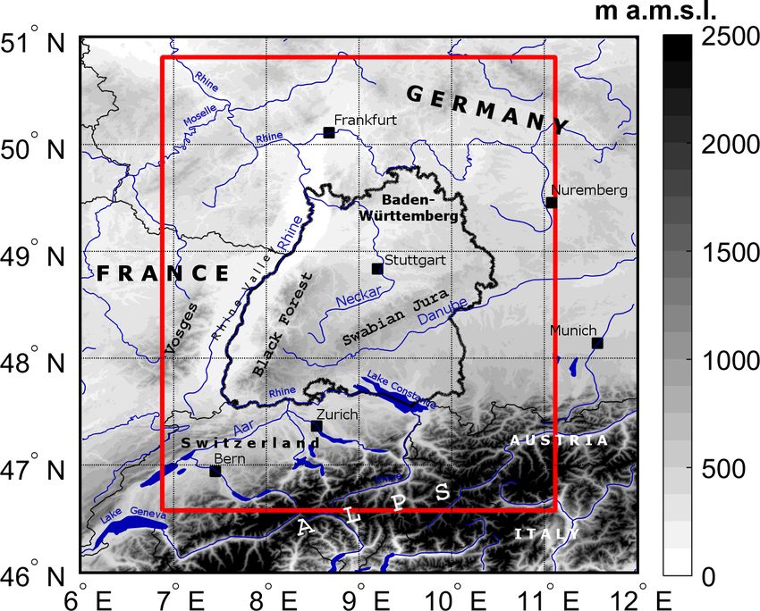
F. Ehmele and M. Kunz: Stochastic precipitation model                                                                             1085

                                                                       ciated with synoptic-scale fronts and Rconv related to em-
                                                                       bedded convection atop stratiform clouds on a local scale
                                                                       (e.g., Fuhrer and Schär, 2005; Kirshbaum and Smith, 2008).
                                                                       While the former component can modify the entire precipi-
                                                                       tation field, the latter can lead to enhanced totals on the local
                                                                       scale. Deep moist convection, however, is not considered, as
                                                                       it is not relevant for larger river floods. Note that both Roro
                                                                       and Rfront can attain negative values in descent areas. Neg-
                                                                       ative values of total precipitation Rtot , however, are physi-
                                                                       cally not meaningful and are therefore truncated away (i.e.,
                                                                       Rtot = max(Rtot , 0) in Eq. 1).

                                                                       2.2     The Smith–Barstad model (SBM)

                                                                       The linear orographic SBM (Smith and Barstad, 2004;
                                                                       Barstad and Smith, 2005) is a simple yet efficient way of
                                                                       computing precipitation over complex terrain. It has been
Figure 1. Topographic map (in meters above mean sea level;             successfully applied in various regions around the world,
m a.m.s.l.) of southwestern Germany and surrounding areas with         e.g., several locations in the US (Barstad and Smith, 2005),
main river networks and lakes as well as substantial orographic        Iceland (Crochet et al., 2007), southwestern Germany (Kunz,
structures. The national borders (slim solid black contours) and the   2011), or southern and northern Norway (Caroletti and
border of the federal state of Baden-Württemberg (bold solid black     Barstad, 2010; Barstad and Caroletti, 2013).
contour) are shown, as well as the model domain (red box), which
extends from 46.6 to 50.8◦ N and from 6.9 to 11.1◦ E.                  2.2.1    Orographic precipitation

                                                                       The SBM is based on the linear theory of three-
2.1   General description
                                                                       dimensional (3-D) stratified, hydrostatic flow over mountains
Overall, the model SPM2D quantifies total precipitation Rtot           with uniform incoming horizontal wind speed and stability
from the linear superposition of four terms, each of them rep-         (Smith, 1980, 1989). It explicitly considers linear flow ef-
resenting a specific precipitation process:                            fects evolving over mountains, such as upstream-tilted grav-
                                                                       ity waves or a flow that goes around rather than over an obsta-
Rtot = Roro + R∞ + Rfront + Rconv .                             (1)    cle in the case of low wind speed, high static stability, and/or
                                                                       large mountains (i.e., small Froude numbers). It is assumed
The first two components of Eq. (1) originate from the di-             that saturated lifting produces condensed water that falls to
agnostic linear model of orographic precipitation according            the ground after a certain time shift (Jiang and Smith, 2003).
to Smith and Barstad (2004) and Barstad and Smith (2005),              Thus, precipitation on the ground is directly related to the
hereafter referred to as the Smith–Barstad model (SBM). The            condensation rate.
first component, Roro , quantifies rain enhancement as a con-             One of the key components of the linear model is a pair
sequence of orographically induced lifting. Over complex               of linear steady-state equations for the advection of verti-
terrain and for high amounts of incoming water vapor flux              cally integrated cloud water and hydrometeor density dur-
(Kunz, 2011), this part dominates the other three in Eq. (1).          ing characteristic timescales of cloud water conversion τc and
The next term, R∞ , is the background precipitation re-                the fallout of hydrometeors τf , respectively. Both timescales
lated to synoptic-scale lifting. According to the omega equa-          are mathematically analogous and are assumed to be con-
tion, large-scale lifting, preferably occurring downstream of          stant in time and also in space for mesoscale domains. When
troughs (low-pressure systems at higher levels), is the result         the timescales are set to zero, the maximum precipitation is
of three different mechanisms: positive vorticity advection            almost one order of magnitude larger compared to a configu-
increasing with height (or vice versa), maximum of diabatic            ration with, for example, τf = τc = 1000 s (Kunz, 2011).
phase transitions, and maximum of warm air advection. Even                A powerful method for the solution of the advection equa-
though vertical lifting results from the superposition of these        tions for cloud physics together with 3-D flow is to apply
three mechanisms, we do not split R∞ accordingly, as the               a two-dimensional (2-D) Fourier transform. Precipitation at
single forcing terms cannot be estimated from vertical sound-          the ground is obtained via an inverse FFT given by the trans-
ings used as input data in our approach (see Sect. 3.2).               fer function:
   As the SBM does not reliably reproduce the observed spa-
tial variability of precipitation also over flat terrain for phys-
ical reasons (Kunz, 2011), we have implemented two ad-
ditional components: Rfront to consider precipitation asso-

www.hydrol-earth-syst-sci.net/23/1083/2019/                                         Hydrol. Earth Syst. Sci., 23, 1083–1102, 2019
1086                                                                  F. Ehmele and M. Kunz: Stochastic precipitation model

                 ZZ
                               iCw σ ĥ(k, l)
Roro (x, y) =
                      (1 − imHw ) (1 + iσ τc ) (1 + iσ τf )
            · ei(kx+ly) dkdl,                                 (2)

which connects the precipitation field in Fourier space (frac-
tion term) to the orography, ĥ(k, l), both related to the hor-
izontal wavenumbers (k, l); i is the imaginary unit, and
Cw = ρSref 0m γ −1 is the uplift sensitivity related to the con-
densation rate ρSref = ρd qv , where ρd is the density of dry air,
qv is the water vapor density, and 0m and γ are the moist adi-
abatic and actual lapse rates, respectively. The scaling height
Hw is the (absolute) height where the integrated water va-
por density dropped to e−1 , and σ = U k + V l is defined as         Figure 2. Probability of observed 24 h rainfall totals greater
the intrinsic frequency with the components U and V of the           than 50 mm, expressed as the average days per year for Baden-
undisturbed horizontal wind vector assumed to be constant            Württemberg; the black box indicates the area where background
through time and space.                                              precipitation R∞ is estimated.
   Whereas the nominator of Eq. (2) gives the dependency
of precipitation on vertical motion and orography, the first
bracket of the denominator describes the modification of the         2.2.2    Background precipitation
source term by airflow dynamics. The second and third terms
                                                                     Under the assumption that the prevailing synoptic conditions
of the denominator consider the advection of hydrometeors
                                                                     during the 12 h of model integration are approximately hori-
during the characteristic timescales τx (x = c; f ). In case of
                                                                     zontally homogeneous and stationary, R∞ also becomes con-
a descent downstream of mountains, Roro may become nega-
                                                                     stant. To consider large-scale lifting in the SPM2D, we esti-
tive, leading to a reduction of total precipitation in Eq. (1) in
                                                                     mate R∞ from observed rainfall totals (see Sect. 3.1) over
that area.
                                                                     a larger area with almost flat terrain, where Roro as well as
   The vertical wavenumber m in Eq. (2) is given by the dis-
                                                                     evaporation associated with an ascent are minimized to a
persion relation (Smith, 1980):
                                                                     large degree. To ensure proper estimation of R∞ for the his-
                                    0.5                             toric events, we choose an area that covers most of the total
                Nm2 − σ 2  2 2

m(k, l) =                  k +l            .                  (3)    investigation area but excludes the Black Forest and the pre-
                   σ2                                                Alpine region, where precipitation totals are highest. In the
In this formulation, m controls both the depth and tilt of a         selected region (Fig. 2, black box), large totals occur only
forced ascent or descent. Because vertical lifting is assumed        rarely. Values of more than 50 mm per day, for example, ex-
to be saturated throughout the whole column, meaning that            hibit an annual exceedance probability p of less than 0.5.
the lifted condensation level (LCL) is directly at the ground,       Furthermore, as confirmed by Fig. 2, the probability of rain
so the saturated Brunt–Väisälä frequency Nm (e.g., Lalas and         totals in excess of 50 mm per day is more or less homoge-
Einaudi, 1973) has to be considered instead of the dry one,          neously distributed.
Nd . Compared to unsaturated conditions, saturated flow leads
                                                                     2.3     Modifications of the SBM
to a weakening of the amplitude of the gravity waves via the
reduction of static stability. In this case, the flow tends to       As further development, two types of modifications are ap-
go more directly over an obstacle rather than around (Dur-           plied to the SBM: adjustments to the existing orographic
ran and Klemp, 1982; Kunz and Wassermann, 2011). Even                precipitation using additional calibration parameters and ad-
though the concept of saturated flow by simply consider-             ditional precipitation components originating from different
ing Nm must be regarded as an approximation of the real-             physical processes.
ity, it has been successfully applied by several authors study-
ing flow dynamics and precipitation (Jiang and Smith, 2003;          2.3.1    Adjustments to Roro
Smith and Barstad, 2004; Kunz and Wassermann, 2011).
   Combining Eq. (2) with Eq. (3), a total number of seven           The original orographic precipitation equation of the SBM
atmospheric parameters is required as input for Roro . In this       (Eq. 2) is modified in the SPM2D by adding three constant
study, we used vertical profiles of temperature, moisture, and       calibration parameters (bold symbols):
wind from radio soundings (see Sect. 3.2) for that purpose.

Hydrol. Earth Syst. Sci., 23, 1083–1102, 2019                                      www.hydrol-earth-syst-sci.net/23/1083/2019/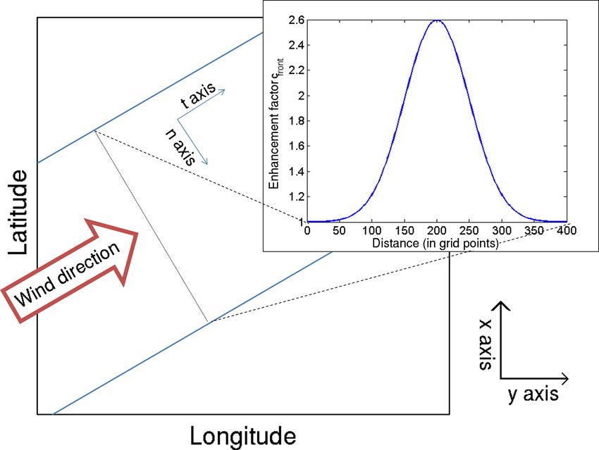
F. Ehmele and M. Kunz: Stochastic precipitation model                                                                               1087

                                                                         2.3.2   Frontal precipitation

                                                                         Apart from large-scale lifting connected to low-pressure sys-
                                                                         tems or waves in the flow patterns, precipitation is also sub-
                                                                         stantially enhanced by synoptic-scale weather fronts. Active
                                                                         fronts may increase precipitation considerably due to cross-
                                                                         frontal circulations and lifting in the warm sector of a cyclone
                                                                         (e.g., Bergeron, 1937; Eliassen, 1962). Conversely, if a front
                                                                         affects only parts of the investigation area (e.g., in case of
                                                                         a trailing front, where the flow is almost parallel to the iso-
                                                                         bars), regions not affected by the front experience much less
Figure 3. Different effects of the implemented internal free param-
eters fdry (blue), fCw (red), and coro (green) on the original oro-      or even no rain at all. Both effects are considered by a sim-
graphic precipitation part (black curve) for a west-to-east cross sec-   plified parameterization Rfront in Eq. (1):
tion through the model domain. The underlying orography is shown
in black.                                                                Rfront = (Roro + R∞ ) · (cfront − 1) ,                       (5)

                                                                         where cfront serves as an enhancement or reduction factor
                                                                         of the overall precipitation. In this parameterization, Roro is
Roro (x, y) = coro · fdry (x, y)                                         considered again because frontal precipitation is additionally
              ZZ
                            ifCw Cw σ ĥ(k, l)                           enhanced by orography, as shown, for example, by Browning
            ·                                                            et al. (1975) or Houze and Hobbs (1982). Due to the additive
                 (1 − imHw ) (1 + iσ τc ) (1 + iσ τf )
                                                                         superposition of all precipitation components in Eq. (1), we
            · ei(kx+ly) dkdl.                                     (4)    have to subtract the original precipitation totals, leading to a
                                                                         total multiplier of (cfront − 1).
   The uplift sensitivity factor Cw is adjusted by a multi-                 In order to estimate cfront from the observational data, we
plier fCw , which reduces the sensitivity of the SPM2D for               define this quantity as the relative difference between obser-
lifting and, therefore, the precipitation rate. Precipitation is         vations O and output M of the SBM. This is expressed by
reduced the most for sharp height gradients, whereas the ef-                              −1
fect is only weak for smooth terrain (Fig. 3, red curve). The            cfront = O · M        ,                                      (6)
formulation of the SPM2D also allows for multiple ascents
                                                                         assuming that the differences originate primarily from frontal
and/or descents of a virtual air parcel without any changes
                                                                         effects. For the quantification of cfront , we use spatial mean
in its water vapor content. The more realistic partial removal
                                                                         values over the investigation area O and M for a training
of water vapor due to condensation during the ascent is also
                                                                         sample of historic heavy rain events (see Sect. 2.4.1).
considered by implementing the additional function fCw .
                                                                            The frontal enhancement factor is a function of space re-
   An additional parameter, fdry , is implemented in Eq. (4) to
                                                                         alized by a rectangular area cfront (n, t), where the orientation
reduce evaporation in descent regions, where Roro becomes
                                                                         of the front-parallel t axis compared to the zonal-orientated y
negative (Fig. 3, blue curve). The resulting underestimation
                                                                         axis is prescribed by the mean wind direction β (Fig. 4). For
of precipitation is found especially downstream of steeper
                                                                         each time step the maximum value of cfront is estimated using
mountains with a greater descent (Kunz, 2011). The parame-
                                                                         the corresponding PDF (cf. Sect. 5.1). To avoid strong gradi-
ter fdry < 1 only corrects grid points (x, y) where Roro < 0;
                                                                         ents at the borders of the rectangular, we applied Gaussian-
otherwise fdry = 1.
                                                                         shaped smoothing. Along the front-normal n axis, the spread
   Finally, the last additional calibration parameter, coro , re-
                                                                         is set to 8σn , where σn is the standard derivation of the nor-
duces orographic precipitation in the whole domain (Fig. 3,
                                                                         mal distribution; in the t direction, the front is infinitely ex-
green curve). It is a consequence of the assumption that the
                                                                         tended (Fig. 4). As the minimum of cfront is zero, Rfront can
vertical lifting of an air column with overall saturation pro-
                                                                         also attain negative values, leading to a weakening of total
duces condensate and instantaneous fallout at any time, im-
                                                                         precipitation for areas unaffected by a front.
plying an overestimation of precipitable water. In reality, not
all layers are completely saturated, and water may also partly           2.3.3   Embedded convection
be stored by clouds. The parameter coro is assumed to be in-
dependent of any lifting processes and constant in time for              Embedded convection mainly occurs when lifting is locally
the whole domain. From a mathematical perspective, the two               enhanced at mid- and upper-tropospheric levels, leading to a
factors, fCw and coro , could collapse into one single param-            decrease of thermal stability by the release of latent heat of
eter. Nevertheless, as mentioned above, they describe mod-               condensation (e.g., Kirshbaum and Durran, 2004; Kirshbaum
ifications of different physical processes and must therefore            and Smith, 2008; Cannon et al., 2012). Convection in general
remain separate.                                                         involves several complex processes that make reliable simu-

www.hydrol-earth-syst-sci.net/23/1083/2019/                                           Hydrol. Earth Syst. Sci., 23, 1083–1102, 2019
1088 F. Ehmele and M. Kunz: Stochastic precipitation model
Figure 5. Schematic of embedded convection implementation by
Figure 4. Schematic of a Gaussian-shaped distribution of the frontal
using rectangular cells (blue). The orientation is defined by the wind
enhancement factor with a maximum of cfront = 2.6 and σn = 50
direction (arrow); each cell is assigned to an individual factor cconv .
(upper right corner), and its location in the model domain for a
southwesterly wind direction (arrow). The blue lines indicate the
boundaries of the frontal zone.
footprints in the model. The complete convective precipita-
tion field for each time step is spatially smoothed to avoid
lations a difficult task. Since our model is restricted to large- sharp gradients. For this, we applied a moving average of
scale precipitation with the objective of quantifying extremes 10 grid points to preserve the high spatial variability of con-
of areal precipitation solely, we treat embedded convection vection.
in a very simplified way by implementing several rectangu-
lar cells as convective footprints, similar to the approach for 2.4 Pre-preparation and simulation procedure
the fronts.
Because embedded convection is mainly induced by oro- 2.4.1 Event definition and statistical distribution
graphic lifting, we implemented a multiplicative factor to the functions
precipitation fields related to both orographic and large-scale
lifting, similar to the frontal part: Stochastic modeling of precipitation events with the SPM2D
is based on appropriate PDFs of all input parameters required
Rconv = cconv · (Roro + R∞ ) , (7) by the model. These PDFs are estimated using an adequate
set of representative past heavy rainfall events. Because the
with the enhancement factor cconv . For each 24-hour simu- characteristics of the ambient conditions and thus the precipi-
lation period, we choose a number of rectangular convec- tation regimes change throughout the year, we seasonally dif-
tive footprints, each with a specified width W and length L, ferentiate the estimated PDFs between spring (March–April–
and distribute them randomly over the whole model domain May – hereafter MAM), summer (June–July–August – JJA),
(Fig. 5). The dimensions for each rectangle are estimated autumn (September–October–November – SON), and winter
from the PDFs of historic footprints of deep moist convec- (December–January–February – DJF).
tion (see Sect. 3.3). Furthermore, we restricted the two pa- In the first step, a sufficient and appropriate subset of rele-
rameters to L > W and Lmax = 300 km, or 300 grid points. vant historic events was identified. Here, an event is defined
As for the frontal systems, the wind direction defines the ori- as a period of 1 or more days with persistent precipitation
entation of the longer sides of the rectangles. For each foot- above a certain threshold of daily totals. An extension to
print, we choose a number of L · W specific factors, cconv , multi-day events is reasonable for considering time delays in
with cconv ∈ {0; 1}. As found, for example, by Fuhrer and discharge response or flood waves traveling along river net-
Schär (2005) or Cannon et al. (2012), embedded convection works (e.g., Duckstein et al., 1993; Uhlemann et al., 2010;
can enhance precipitation up to 200 %, but only locally. Thus, Schröter et al., 2015).
the given range of cconv is adequate. Within the single rectan- We define the historic event set according to maximum
gles, the spatial distribution of cconv randomly varies between areal precipitation. For this, we simply accumulate the
the given limits to account for the high spatial variability of (equidistant) 24 h rainfall totals R BW of all grid points in the
convective precipitation. investigation area (BW; see Sect. 3.1). Following the sort-
As embedded convection occurs several times a day and ing of all values of R BW in descending order, the strongest
at several locations, we used a variable number of convective 200 values enter the sample (top200). As precipitation is not
Hydrol. Earth Syst. Sci., 23, 1083–1102, 2019 www.hydrol-earth-syst-sci.net/23/1083/2019/F. Ehmele and M. Kunz: Stochastic precipitation model 1089
limited to these (single) days but may be embedded in longer for the same period. In contrast, Rfront and Rconv are calcu-
time periods, we define the threshold Rthres for the event def- lated only for 24 h as they become apparent as footprints in
inition. For estimating Rthres , we consider “wet” days by us- daily totals. The resulting total precipitation Rtot has a tem-
ing R BW > 0 solely and set Rthres to the 75 % percentile of poral resolution of 24 h. Despite the fact that the character-
this subsample. A lower threshold leads to an overinterpre- istic timescales may vary from one situation to another, it is
tation of longer clusters, and a higher one avoids multi-day found that simulations using fixed values for the free param-
events. eters yield trustworthy results (e.g. Barstad and Smith, 2005;
Event precipitation starts on the first day that ex- Kunz, 2011). Here, we also use constant values illustrated as
ceeds Rthres . When areal means of consecutive days are also the shaded box in Fig. 6. The direct link between the pre-
above Rthres , they are simply accumulated, yielding events cipitation components and the corresponding input variables
of more than 1 day. The last day with R ≥ Rthres before a (described by appropriate PDFs) is also shown in Fig. 6. In
period of at least 3 three days of non-exceedance defines case t < tev , the next 24 h period is simulated; otherwise, the
the end of an event. Such a 3-day period ensures statisti- loop jumps to the next event. A method how to assign the
cal independence of the events in accordance with the ap- nE events to a specific time period, which is required, for ex-
proach of Palutikov et al. (1999) for wind storms. Following ample, for insurance purposes, will be introduced in Sect. 6.
Piper et al. (2016), we only count “rain days” (R BW ≥ Rthres )
and neglect “skip days” (R BW < Rthres ) within the start-day
and end-day period for event duration estimation, which is 3 Data sets
a widely used approach (Wanner et al., 1997; Petrow et al.,
2009). This approach avoids the overinterpretation of longer The SPM2D presented in this study is based on two differ-
clusters. Based on this procedure, a defined precipitation ent types of data sets: gridded precipitation data also used to
event contains 1 or more days of the top200 sample. For this calibrate and verify the model and vertical profiles from ra-
event set, all required input parameters were extracted from diosondes to initialize the model. Furthermore, the SPM2D
sounding data and rainfall totals (see Sect. 3). is also validated using reanalysis.
In the next step, we identified the PDFs most appropriate
3.1 Rainfall totals
for statistically describing each of the seven atmospheric in-
put parameters, the event duration tev , background precipita- Rainfall statistics in our study are based on the regional-
tion R∞ , and front factor cfront . In addition to 20 PDFs preset ized precipitation (REGNIE) data provided by the German
by the MATLAB statistical toolbox (MATLAB, 2016), we Weather Service (DWD). REGNIE is a gridded data set of
considered the circular von Mises distribution (Mardia and 24 h totals (06:00 to 06:00 UTC) based on several thousand
Zemroch, 1975) for wind direction only. In Sect. 5 it will be climate stations more or less evenly distributed across Ger-
further discussed which PDFs are most suitable for the input many (so-called RR collective). The REGNIE algorithm in-
variables in our case. terpolates the observations to a regular grid of 1 km2 consid-
To find the PDF that best fits the data, we estimated the ering elevation, exposition, and climatology (Rauthe et al.,
appropriate number of histogram classes according to Freed- 2013). Despite of continuous changes in the number of sta-
man and Diaconis (1981) and calculated bias, the root-mean- tions considered and several station relocations, REGNIE is
square error (RMSE), and the Spearman correlation coeffi- sufficiently homogeneous for our purposes. However, areal
cient rSp (Spearman, 1904) as quality indicators (QIs). We precipitation exhibits a certain bias, especially over elevated
also applied a χ 2 test (Wilks, 2006) as a QI. For each QI, we terrain, such as the peaks of the Black Forest, where the num-
ranked the PDFs in ascending order and added up the rank ber of stations is very limited (Kunz, 2011).
numbers for each PDF, receiving the best fit in terms of the In our study, we use REGNIE data from 1951 to 2016 to
least QI rank sum (QIRS). In the case of alikeness of two or identify the top200 event set (see previous section); to esti-
more PDFs (about 10 % of all cases), we manually selected mate the duration of the events, the front factor cfront , and
the best one. background precipitation; and to validate the SPM2D simu-
lation results.
2.4.2 General simulation procedure
3.2 Radio soundings
The presented SPM2D is an event-based model in the sense
that a specified number nE of independent events with vari- The seven input parameters (see Sect. 2) required by the
able duration tev is simulated. The general procedure is as SPM2D model are derived from vertical profiles (00:00 and
follows (cf. Fig. 6). Starting with the iteration loop over 12:00 UTC) of temperature, moisture, wind speed, and direc-
nE events, the season and duration tev are set at first. The next tion at the radio sounding station of Stuttgart located some-
step is the simulation of the four precipitation components what downstream of the northern Black Forest. Even though
according to Eq. (1); because radio soundings used as in- the location might not be ideal because the profiles do not
put data are available every 12 h, Roro and R∞ are computed represent undisturbed conditions, the profiles are similar to
www.hydrol-earth-syst-sci.net/23/1083/2019/ Hydrol. Earth Syst. Sci., 23, 1083–1102, 20191090 F. Ehmele and M. Kunz: Stochastic precipitation model
Figure 6. Flow chart of the individual components of the SPM2D (solid boxes) and the corresponding input variables (PDFs; dashed boxes).
Loops are highlighted as ellipsis or bold dashed arrows. The constant model parameters are illustrated as the shaded box.
those of the upstream station of Nancy in France, as shown bourg between 2005 and 2014 were identified from the con-
by Kunz (2011) for heavy rainfall events on average. Data stant altitude plan position indicator (CAPPI) for a reflectiv-
from Nancy are available after 1990 only and, thus, cannot ity in excess of 55 dBZ. The application of the tracking algo-
be used in this study, whereas soundings from Stuttgart have rithm TRACE3D (Handwerker, 2002) identified more than
been available since 1957. 25 000 storm tracks. Even though we do not consider rain-
The vertical profiles, provided by the Integrated Global fall related to severe convective storms in the SPM2D, the
Radiosonde Archive (IGRA) from the National Climatic statistical distributions of the storm’s dimensions are reliable
Data Center (Durre et al., 2006), were interpolated into proxies for the extension of enhanced precipitation from em-
equidistant increments of 1z = 10 m (Mohr and Kunz, bedded convection described by Rconv .
2013). All derived environmental parameters refer to the low-
est 5 km of the atmosphere since this layer is most relevant 3.4 Numerical weather simulations
for airflow and stability. Furthermore, to account for the de-
creasing impact of higher atmospheric layers on the flow The SPM2D simulation results are additionally validated
characteristics, the flow parameters 3 are integrated verti- with high-resolution reanalysis from the non-hydrostatic
cally (3),
e applying water vapor weighting (Kunz, 2011): Consortium for Small-scale Modeling (COSMO) model in
climate mode (CCLM; Rockel et al., 2008). Natalie Laube
Rzt (Institute of Meteorology and Climate Research, Karlsruhe
3ρd qv dz
z=0
Insitute of Technology, personal communication, 2018) per-
3
e= , (8) formed a dynamical downscaling of an ERA-40 reanalysis
Rzt
ρd qv dz from the European Centre for Medium-Range Weather Fore-
z=0 casts (ECMWF; Kållberg et al., 2004) to a horizontal res-
olution of 2.8 km for southern Germany using a 3-fold re-
where ρd is the density of dry air and zt is the upper inte-
gional nesting (50 km, over 7 km, to 2.8 km). High-resolution
gration limit, here of 5000 m. As some layers may be moist-
CCLM data are available for the period 1971–2000. For the
unstable, resulting in imaginary Nm , the averaging routine is
evaluation, we considered the top200 REGNIE events from
applied to Nm2 . In the few cases where Nem was imaginary, it
which around 100 events occurred within the CCLM period,
was set to a near-neutral, constant value of 0.0003 s−1 .
including the top two events, seven of the strongest 10 events
3.3 Parameters for embedded convection or 14 of the strongest 20 events.
The stochastic generation of enhanced precipitation streaks
associated with embedded convection, namely their length
and width (L and W ), relies on the statistics of severe con-
vective storms in Germany (Fluck, 2018). In that study, con-
vective storms in Germany, France, Belgium, and Luxem-
Hydrol. Earth Syst. Sci., 23, 1083–1102, 2019 www.hydrol-earth-syst-sci.net/23/1083/2019/F. Ehmele and M. Kunz: Stochastic precipitation model 1091
Table 1. Range of values of the free model parameters used for the 4.2 Calibration results
calibration of the model.
Applying the method as described above, the highest value
Parameter Minimum Maximum Increment for S = 0.60 as the median of all top200 events is ob-
τx 800 s 1500 s 100 s tained for the combination of τx = 1400 s, fCw = 1.0, fdry =
fCw 0.5 1.0 0.1 0.4, and coro = 0.8. For this combination, the median val-
fdry 0.4 1.0 0.1 ues of the other quality indices are rSp = 0.39, σ̂f = 0.98,
coro 0.5 1.0 0.1 bias = 6.30 mm, and RMSE = 14.85 mm. The assessed value
for τx is physically plausible and comparable to other studies
with the SBM (e.g., Barstad and Smith, 2005; Caroletti and
4 Calibration Barstad, 2010; Kunz, 2011). Considering the slight overes-
timation of orographic precipitation and the strong overesti-
4.1 Method mation of drying in the lee of the mountains by the SBM,
the values for those adjustments are also physically plausi-
The SPM2D is calibrated with the top200 events (training ble. Note that the parameter combination identified above
data) by adjusting the free model parameters τx , fCw , fdry , yields the lowest errors only when averaging over all top200
and coro (cf. Sect. 2) and comparing the simulation results events. Single events are more realistic with another param-
with observations. The parameter combination yielding the eter combination, reflecting particularly the unknown, and
best simulation results is then used for the stochastic simula- thus not considered microphysical processes that are deci-
tions (validation data). The components Rfront and Rconv are sive for precipitation formation strongly controlled by ver-
only considered for the stochastic event set and are therefore tical wind speed, temperature, and moisture profiles. The
neglected here. In this configuration, the SPM2D is equiva- dependency of microphysical processes on ambient condi-
lent to the SBM plus our modifications in Roro , referred to as tions, however, is not relevant when running the model in the
the SBM + M. stochastic mode, which is the objective in this study.
In order to determine appropriate values of the free pa- The sensitivity of the skill score S to changes in τ , fCw ,
rameters, a large number of model simulations were carried and coro (Fig. S1 in the Supplement) shows a kind of dipole
out. Whereas one parameter was successively varied, the oth- structure in both cases with the highest values of S along
ers were kept constant. The selected ranges and increments the counter diagonal. Lower values for S are obtained for the
of the parameters listed in Table 1 resulted in 2016 possible shortest (longest) timescales in combination with the high-
parameter combinations, giving a total number of approx- est (lowest) uplift sensitivity or highest (lowest) weighting
imately 390 000 simulation days for the top200 event set. of Roro in Eq. (1). This means that horizontal precipitation
Both data sets (from SBM + M and REGNIE) are slightly drift over short distances also reduces evaporation, leading
smoothed using a running 5 × 5 grid box, as the REGNIE to an overestimation of orographic precipitation (and vice
data show a certain spatial uncertainty (cf. Sect. 3.1), espe- versa). This effect has to be considered by adjusting Roro .
cially around the crests of the Black Forest. Furthermore, as
shown, for example, by Barstad and Smith (2005), smoothed 4.3 Sensitivity of simulated total precipitation
data yield more robust results when comparing model and
observation data. Note, however, that larger values of τx and To demonstrate how variations of atmospheric conditions
smaller values of fCw similarly smooth the simulated precip- translate into precipitation, we conduct a sensitivity study
itation fields. In these cases, the QIRS method used for the with the SBM + M using the top200 event set by gradually
evaluation (Sect. 2.4.1) has to be applied carefully. changing the values of the input parameters. Following Kunz
The model skill was evaluated using the skill score S ac- (2011), we perturbed the values of Nm2 , qv , U , β, and τ . This
cording to Taylor (2001) (see Eq. A1 in the Appendix) to is done by multiplying the respective quantity with var_mult
determine the best combination of the free model param- increasing linearly from 0.5 to 2.0 in increments of 0.1. Wind
eter. S relies on the Spearman (1904) correlation coeffi- direction β is varied in the range of ±30◦ in increments of 5◦ .
cient rSp between the SBM + M simulations and the obser- The calibration parameters are set to their optimum values
vations (REGNIE) as well as on the standard deviations σ of estimated in the previous section. Besides areal mean precip-
both data sets. The skill score S is computed for each day of itation, we computed RMSE and skill score S for the median
the top200 and each parameter combination. From all real- of the top200 event set.
izations, we select the parameter combination that yields the Mean precipitation shows a high sensitivity to changes
highest median value of S averaged over the top200, as the in qv , U , and β (Fig. 7). In all cases, precipitation increases
SPM2D should be able to properly represent a broad range with increasing values and decreases with decreasing values.
of different atmospheric conditions. Lowest sensitivity occurs for β between ±15◦ because of
the orientation of the major orographic structures (i.e., the
Black Forest) from southwest to northeast. Westerly inflow,
www.hydrol-earth-syst-sci.net/23/1083/2019/ Hydrol. Earth Syst. Sci., 23, 1083–1102, 20191092 F. Ehmele and M. Kunz: Stochastic precipitation model
4.4 Case study
After the parameter adjustment, the SBM + M tends to
slightly underestimate orographic precipitation, whereas to-
tals over flat or rolling terrain are overestimated. This behav-
ior can be seen for the case study of 31 May 2013 (Fig. 8),
a heavy precipitation event that triggered the severe flooding
in 2013 (Schröter et al., 2015).
On that day, a pronounced low-pressure system with its
center over Croatia led to the sustained advection of moist
air masses from northerly directions around 20◦ in com-
bination with a synoptic-scale ascent. The Stuttgart sound-
ing showed low stability (Nm = 0.0055 s−1 ), high precip-
itable water (pw = 24 kg m−2 ), and high wind speed (U =
20 m s−1 ), which is already an indication of heavy rainfall.
Consequently, precipitation totals across the investigation
Figure 7. Areal mean precipitation (24 h totals; median of the area reached values of 10–100 mm.
top200 event set) as a function of Nm 2 , q , U , β, and τ , perturbed by
v Overall, the SBM + M is able to reproduce most of
a multiplicative factor (0.5 ≤ var_mult ≤ 2) and changed 1β. The
the structures of the observed rain field (Fig. 8), espe-
dotted lines indicate the values of the reference run.
cially the location of the maxima. The observed mean for
Baden-Württemberg is R obs = 33.1 mm, whereas the sim-
prevailing on average, still occurs for small variations of β. ulated mean is R mod = 37.3 mm, thus being only 12.6 %
For greater shifts (1β > 20◦ or 1β < −20◦ ), when the in- higher compared to the observations. Maximum values are
flow angle becomes smaller, the sensitivity slightly increases. Rmax,obs = 91.7 mm and Rmax,mod = 76.3 mm, which is a de-
The changes in the wave regimes, and thus the location of viation of about 17 %. The area with R ≥ 50 mm is almost
the updraft, may also explain the partly stepwise form of the equal with slightly less grid points (≈ 6 %) in the SBM + M.
curves for both β and U . The results for Nm2 and τ reveal The best agreement is found for the northern Black Forest as
the opposite behavior with an increase in precipitation for well as the Swabian Jura. Over the northern part of the model
smaller values and vice versa. Furthermore, the sensitivity of domain (north of 49◦ N) and southwest of Stuttgart, sim-
the SBM + M to changes in these two parameters is much ulated rainfall is substantially higher compared with REG-
weaker compared to the other parameters. NIE. In contrast, the SBM + M simulates lower totals in the
Qualitatively similar behavior to the model is found for southern Rhine Valley near and over the mountainous re-
the medians of RMSE and skill score S (Fig. S2). While gions of the southern Black Forest (around Freiburg), es-
areal precipitation only provides insights into how changes pecially east of the city of Basel, where lee-side evapora-
in the ambient parameters feed back into rainfall, RMSE tion in the model dominates. The quality indices for that
and S also consider the spatial distribution. The results for day are S = 0.62, rSp = 0.30, σ̂f = 0.75, bias = 4.44 mm, and
RMSE (Fig. S2a) again reveal the highest sensitivity of the RMSE = 14.82 mm.
SBM + M to changes in qv and U . While for var_mult > 1, One reason for the discrepancy between observed and sim-
the sensitivity in terms of RMSE is similar to areal precip- ulated precipitation might be the suboptimal location of the
itation, there is a much higher sensitivity for var_mult < 1. Stuttgart sounding used for the model initialization. The sen-
In those cases, orographic precipitation is more detached to sitivity study as described in Sect. 4.3 for this particular event
the mountain crests, resulting in higher totals due to reduced obtains the best results in terms of the lowest RMSE (Fig. 9)
evaporation in the descent regions. Because of the combina- for an increase in Nm2 or τ , whereas in the case of qv or U , the
tion of higher totals at different locations, RMSE shows a lowest RMSE is obtained when decreasing the original val-
higher sensitivity to changes in τ and Nm2 compared to areal ues. Regarding β, the lowest RMSE is given for the original
mean precipitation. value. The highest skill score S, conversely, is reached for in-
The skill score S, in contrast, is most sensitive to changes creasing U and qv and decreasing τ and Nm2 . In the case of β,
in qv and τ (Fig. S2b). Regarding Nm2 , S decreases just for S continuously decreases from 0.8 for northwesterly inflow
very high values of var_mult, while there is almost no sensi- to 0.4 for northeasterly winds.
tivity on β. In all cases, highest S is obtained for the original
values of the input parameters, confirming that the model is
well calibrated.
Hydrol. Earth Syst. Sci., 23, 1083–1102, 2019 www.hydrol-earth-syst-sci.net/23/1083/2019/F. Ehmele and M. Kunz: Stochastic precipitation model 1093
Figure 8. Comparison of (a) REGNIE 24 h rainfall totals, and (b) SBM + M output for southwestern Germany for the case study on
31 May 2013. Note that REGNIE data are available for Germany only. The parameterization in (b) is τx = 1400 s, fCw = 1.0, fdry = 0.4,
and coro = 0.8. The areas outside of Baden-Württemberg are white for better visualization and comparison.
Table 2. Estimated best-fitting PDFs for event duration (tev ), back-
ground precipitation R∞ , and frontal enhancement factor cfront de-
rived from REGNIE data (top box); square of saturated Brunt–
Väisälä frequency Nm 2 , wind direction β, horizontal wind speed U ,
scaling height Hw , actual lapse rate γ , saturated moist adiabatic
lapse rate 0m , and condensation rate ρSref derived from sounding
data (bottom box). For the PDF acronyms, see Table A1.
Model parameter MAM JJA SON DJF
tev GEV GEV BSD NkD
R∞ WbD WbD WbD WbD
cfront LND GmD LND ND
Nm2 GEV GbD GEV GEV
β GEV GEV GEV SD
U HND IGD HND GEV
γ GEV GEV IGD IGD
0m GEV IGD IGD GEV
Hw GEV GbD GEV LD
ρSref WbD GEV WbD WbD
PDF that best fits the distribution of the observations (Ta-
ble 2) by using the least QIRS method (cf. Sect. 2.4.1). From
the overall 21 PDFs that were considered, only 12 turned
Figure 9. Changes in (a) RMSE, and (b) skill score S for per- out to be suitable for adjusting the observations. In most of
turbed values of Nm 2 , q , U , β, and τ , with a multiplicative fac-
v
the cases, the generalized extreme value distribution (GEV),
tor (var_mult), and changed 1β, for 31 May 2013. The dotted lines with its special realizations of the Gumbel distribution (GbD)
indicate the values of the reference run. and Weibull distribution (WbD), appears to be appropri-
ate (26 cases), followed by the inverse Gaussian distribu-
tion (IGD) for five parameters and the Gamma distribu-
5 Parameter estimation of the stochastic simulations tion (GmD) for three parameters. Especially for flow param-
eters derived from the soundings, the GEV appears to be the
5.1 Adjustment of the PDFs most appropriate (19 out of 28 cases). We had to choose the
PDF manually 5 times due to the alikeness of two PDFs ac-
After separating the historic event set into the four main sea- cording to the QIRS method.
sons, we estimate, for each of the 10 input parameters, the
www.hydrol-earth-syst-sci.net/23/1083/2019/ Hydrol. Earth Syst. Sci., 23, 1083–1102, 20191094 F. Ehmele and M. Kunz: Stochastic precipitation model
Concerning R∞ , totals of 20–25 mm day−1 are found to
most likely occur within a range of 3–37 mm day−1 in DJF,
3–50 mm day−1 in JJA, and 0–50 mm day−1 during the other
two seasons (not shown). The corresponding PDFs are listed
in Table 2. For the cfront parameter, all PDFs have their max-
imum around 0.7 to 0.8, with a range from 0.4 to 1.4 for
most of the seasons (not shown). The distribution in SON
(Table 2) descends slower towards higher values (maximum
of around 1.6).
5.3 Atmospheric parameters
An overview of the range of the seven input parameters of
the model is shown as box plots in Fig. 11; the correspond-
ing PDFs are listed in the bottom box of Table 2. In most
cases, the atmosphere was slightly stably stratified, as rep-
resented by positive values of Nm2 affecting the wave prop-
Figure 10. Histogram of top200 event duration for Baden- agation. During JJA, the distribution is shifted toward neg-
Württemberg according to REGNIE (bars), and estimated best- ative values (unstable; recall that negative values are set to
fitting PDFs (dotted lines) for the summer (blue) and the winter Nm = 0.0003 s−1 ), whereas in DJF, there are almost entirely
(red). positive values. Wind direction β, decisive for the spatial dis-
tribution of precipitation around the mountains, shows pro-
nounced seasonal differences. More than 90 % of the top200
The input parameters are considered as independent and DJF events have southwesterly to northwesterly winds (240–
uncorrelated. To justify this assumption, we performed a cor- 300◦ ), with other directions hardly observed. The reason is
relation analysis of all possible combinations of input param- that northerly flows are usually associated with low temper-
eters using the Spearman (1904) correlation coefficient. A atures and thus low humidity during DJF. In JJA, the wind
low number of about 16 % of the parameters have a corre- direction that occurred most frequently is between 240 and
lation coefficient above ±0.5, and only 4 % are highly cor- 300◦ as well. However, all other directions have been ob-
related with ±0.7. Regarding these cases, 90 % show nega- served as well.
tive correlations with r ≤ −0.5. However, there are distinct Horizontal wind speed U in all cases and all seasons is
seasonal differences; in some cases correlations are higher high, especially during DJF, where reduced moisture is com-
in summer than in winter. The highest correlation exists be- pensated by high velocity to obtain substantial horizontal in-
tween Nm2 and the lapse rates, which is plausible as both coming moisture flow. Median values are 5 and 20 m s−1 dur-
are based on the vertical temperature gradient. Because the ing JJA and DJF, respectively. Flow parameters related to
SPM2D is less sensitive to Nm2 (cf. Sect. 4) the effect can be humidity (Hw , ρSref ) conversely show higher values in JJA,
neglected in the model. where 0m is reduced due to the release of latent heat. The
quantity γ shows similar medians and interquartile ranges
5.2 Event characteristics
with a broader distribution in DJF.
The histogram of the duration tev for the top200 event set
and the corresponding best-fitting PDF, shown exemplary in
Fig. 10, illustrated that during JJA, a duration of 2–3 days 6 Stochastic event set and model validation
dominates, with a decreasing probability toward longer pe-
riods. During DJF, the distribution is generally shifted to Overall, a total number of nE = 10 000 events (equivalent to
longer events, whereas the probability for single-day events approx. 31 500 days) have been simulated with the SPM2D
remains roughly unchanged. The maximum of 15 days in in stochastic mode (see Sect. 2.4.2). Therefore, a stochas-
DJF represents the longest duration of the top200 event set. tic set of input variables with the same size as the number of
Whereas the estimated PDF for the JJA (GEV) has a sharper simulation days was created using the estimated PDFs, where
maximum and a stronger decrease in tev > 3, the PDF found the variables can be treated as independent (cf. Sect. 5.1). For
to best fit the duration in the DJF (NkD) shows a broader the validation of the SPM2D, we quantified statistical met-
range of possible durations. Note that the histogram in the rics such as return periods, probabilities, and percentiles and
winter shows a large scattering with irregular peaks, making evaluated them with observations (REGNIE), CCLM simu-
an adjustment of a PDF difficult. For MAM and SON, the lations, and the SBM + M part. The statistical distribution
results are comparable to those of DJF and JJA, respectively. of the stochastic event set of the SPM2D should agree with
that of the top200 historic events to a large degree, and more
Hydrol. Earth Syst. Sci., 23, 1083–1102, 2019 www.hydrol-earth-syst-sci.net/23/1083/2019/F. Ehmele and M. Kunz: Stochastic precipitation model 1095
ences also arise northeast and southwest of Stuttgart. Never-
theless, all differences are small, of the order of a few per-
cent. The SBM + M shows an overestimation of precipita-
tion over mountainous terrain, while the CCLM simulates
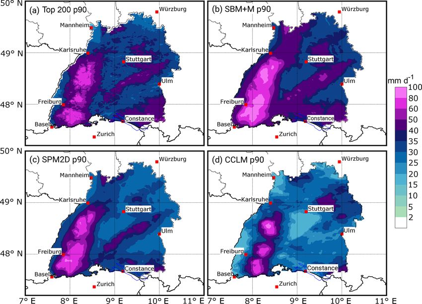
less precipitation overall for the median. For the p90, major
differences appear especially over the rolling terrain.
The areal rainfall of the SPM2D median (Fig. 12) differs
only about 3.3 % from the REGNIE top200, whereas that of
the SBM + M is about 22.1 % higher. The spatial mean of the
CCLM reanalysis is around half of REGNIE, which might be
a result of the reduced sample size. The maximum values at
any grid point of the median field are about 7 % higher in
the SPM2D compared to the REGNIE top200, and are about
34 % higher in the SBM + M realization, whereas the CCLM
maximum is about 44 % smaller.
The areal rainfall for the p90 field (Fig. 13) is about
6.5 % smaller in the SPM2D and about 14 % higher in the
SBM + M, but it is about 22 % smaller in the CCLM. The
maximum values at any grid point of the p90 field are ap-
proximately 1 % smaller in the SPM2D, about 22 % higher
in the SBM + M, and 13 % higher in the CCLM.
Figure 11. Atmospheric parameters required as input for the For other percentiles the differences between REGNIE and
SPM2D derived from radio sounding observations at Stuttgart for the SPM2D are very small for both the spatial mean and the
the top200 events with mean, interquartile distance, minimum, and maximum precipitation at any grid point in the model domain
maximum values; the left whisker of each pair represents the sum- (Fig. S3a). The differences become considerable only above
mer, and the right one represents the winter season. The units for the 95th percentile. The SPM2D tends to overestimate lower
each variable are given in the brackets below the variable names. precipitation amounts because the minimum values at any
grid point are higher in the model than in the observations
and invert for the 99th percentile only. In contrast, the differ-
robust results should be notable at the heavy tail (extreme ences between the SBM + M and REGNIE are considerably
events). The comparison with the SBM + M part is helpful larger for maxima, minima, and spatial means throughout ev-
in highlighting the quality and necessity of the modifications ery percentile. The CCLM reanalysis has a negative deviation
made to the original SBM. High-resolution CCLM simula- for minimum and spatial mean precipitation at all percentiles,
tions are chosen for validation to demonstrate the advantages whereas for the maximum values there is a marked underesti-
of using a statistical approach for stochastic simulations in- mation for lower percentiles and an overestimation at higher
stead of a dynamical NWP model. percentiles. At small percentiles, the QIs, such as rSp , S, or
Spatial 24 h mean values range between 1.2 and 79.7 mm σ̂f , have low values due to the overestimation of the SPM2D
in the SPM2D, and 1.3 to 97.0 mm in the SBM + M, whereas (Fig. S3b). The highest skill is reached around the 90th per-
the maximum for the top200 is only 49.6 mm. In total, centile, with a slight decrease for higher values, which can be
128 events (0.4 %) of the SPM2D or 724 (2.1 %) of the the result of the increasing uncertainties of the observations.
SBM + M yield higher spatial precipitation amounts than the Nevertheless, a skill score of around or above 0.8 confirms
maximum of the top200. The CCLM simulations range be- the reliability of the stochastic simulations.
tween 1.8 and 37.6 mm. To estimate precipitation distributions for specific return
Both the median and the 90th-percentile (p90) precipita- periods, we fit a Gumbel PDF to the annual maximum series
tion fields of the top200 event set and the SPM2D agree of both REGNIE and the SPM2D. As it is not possible to di-
well concerning the spatial distribution and the precipitation rectly estimate the time period and a corresponding annual
amounts (Figs. 12 and 13). Significant orographic precipita- maximum series for the stochastic event set, we count the
tion enhancement over the Black Forest and Swabian Jura is number of stochastic values exceeding the 99th percentile of
clearly visible in all data sets. Note that the more detailed observations np99 and normalize it by the probability of oc-
structure of the REGNIE data results from the regionaliza- currence p99 , yielding the new time period:
tion method and its strong dependency on orography, which np99
should not be overinterpreted. Larger spatial differences be- TSPM = . (9)
p99
tween the different realizations mainly appear in the north-
ern Rhine Valley and to the northeast of the domain for both After sorting the SPM2D realizations in descending order,
the median and the p90, whereas for the latter, some differ- we take the first nT = TSPM values as the annual series of the
www.hydrol-earth-syst-sci.net/23/1083/2019/ Hydrol. Earth Syst. Sci., 23, 1083–1102, 2019You can also read