Spatial variations in CO2 fluxes in the Saguenay Fjord (Quebec, Canada) and results of a water mixing model - Recent
←
→
Page content transcription
If your browser does not render page correctly, please read the page content below
Biogeosciences, 17, 547–566, 2020
https://doi.org/10.5194/bg-17-547-2020
© Author(s) 2020. This work is distributed under
the Creative Commons Attribution 4.0 License.

Spatial variations in CO2 fluxes in the Saguenay Fjord (Quebec,
Canada) and results of a water mixing model
Louise Delaigue1 , Helmuth Thomas2,3 , and Alfonso Mucci1
1 GEOTOP    and Department of Earth and Planetary Sciences, McGill University, 3450 University Street,
Montreal, QC H3A 0E8, Canada
2 Department of Oceanography, Dalhousie University, 1355 Oxford Street, Halifax, NS B3H 4R2, Canada
3 Center for Materials and Coastal Research, Helmholtz-Zentrum Geesthacht, Germany

Correspondence: Louise Delaigue (louise.delaigue@mail.mcgill.ca)

Received: 28 July 2019 – Discussion started: 7 August 2019
Revised: 10 November 2019 – Accepted: 6 December 2019 – Published: 31 January 2020

Abstract. The Saguenay Fjord is a major tributary of the St.     1   Introduction
Lawrence Estuary and is strongly stratified. A 6–8 m wedge
of brackish water typically overlies up to 270 m of seawater.
Relative to the St. Lawrence River, the surface waters of the    Anthropogenic emissions of carbon dioxide (CO2 ) have re-
Saguenay Fjord are less alkaline and host higher dissolved       cently propelled atmospheric CO2 concentrations above the
organic carbon (DOC) concentrations. In view of the latter,      410 ppm mark, the highest concentration recorded in the past
surface waters of the fjord are expected to be a net source      3 million years (Willeit et al., 2019). The oceans, the largest
of CO2 to the atmosphere, as they partly originate from          CO2 reservoir on Earth, have taken up ca. 30 % of the an-
the flushing of organic-rich soil porewaters. Nonetheless, the   thropogenic CO2 emitted to the atmosphere since the begin-
CO2 dynamics in the fjord are modulated with the rising tide     ning of the industrial era (Feely et al., 2004; Brewer and
by the intrusion, at the surface, of brackish water from the     Peltzer, 2009; Doney et al., 2009; Orr, 2011; Friedlingstein
Upper St. Lawrence Estuary, as well as an overflow of mixed      et al., 2019), mitigating the impact of this greenhouse gas on
seawater over the shallow sill from the Lower St. Lawrence       global warming (Sabine et al., 2004). On the other hand, the
Estuary. Using geochemical and isotopic tracers, in combina-     uptake of CO2 by the oceans has led to modifications of the
tion with an optimization multiparameter algorithm (OMP),        seawater carbonate chemistry and a decline in the average
we determined the relative contribution of known source wa-      surface ocean pH by ∼ 0.1 units since pre-industrial times, a
ters to the water column in the Saguenay Fjord, including        phenomenon dubbed ocean acidification (Caldeira and Wick-
waters that originate from the Lower St. Lawrence Estuary        ett, 2005). According to the Intergovernmental Panel on Cli-
and replenish the fjord’s deep basins. These results, when       mate Change (IPCC) “business as usual” emissions scenario
included in a conservative mixing model and compared to          IS92a and general circulation models, atmospheric CO2 lev-
field measurements, serve to identify the dominant factors,      els may reach 800 ppm by 2100, lowering the pH of the sur-
other than physical mixing, such as biological activity (pho-    face oceans by an additional 0.3–0.4 units, a rate that is un-
tosynthesis, respiration) and gas exchange at the air–water      precedented in the geological record (Caldeira and Wickett,
interface, that impact the water properties (e.g., pH, pCO2 )    2005; Hönisch et al., 2012; Rhein et al., 2013). The grow-
of the fjord. Results indicate that the fjord’s surface waters   ing concern about the impacts of anthropogenic CO2 emis-
are a net source of CO2 to the atmosphere during periods of      sions on climate, as well as marine and terrestrial ecosys-
high freshwater discharge (e.g., spring freshet), whereas they   tems, calls for a meticulous quantification of organic and in-
serve as a net sink of atmospheric CO2 when their practical      organic carbon fluxes, especially in coastal environments, in-
salinity exceeds ∼ 5–10.                                         cluding fjords, a major but poorly quantified component of
                                                                 the global carbon cycle and budget (Bauer et al., 2013; Na-
                                                                 jjar et al., 2018). Meaningful predictions of the effects of

Published by Copernicus Publications on behalf of the European Geosciences Union.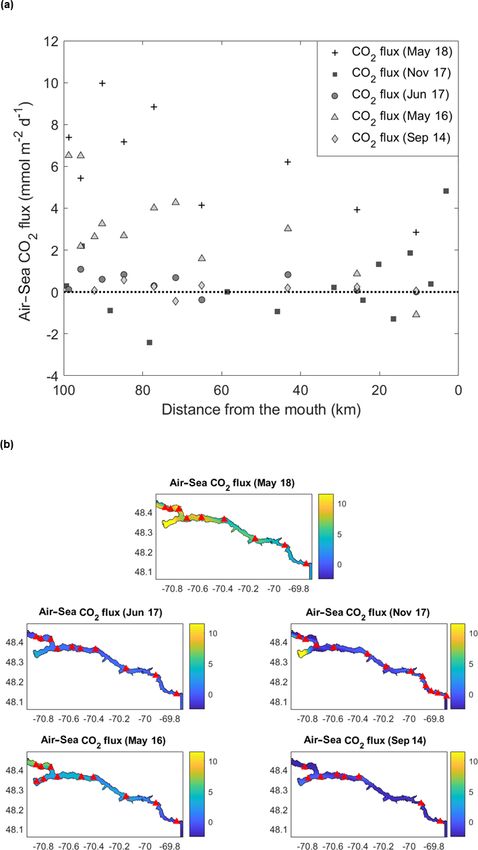
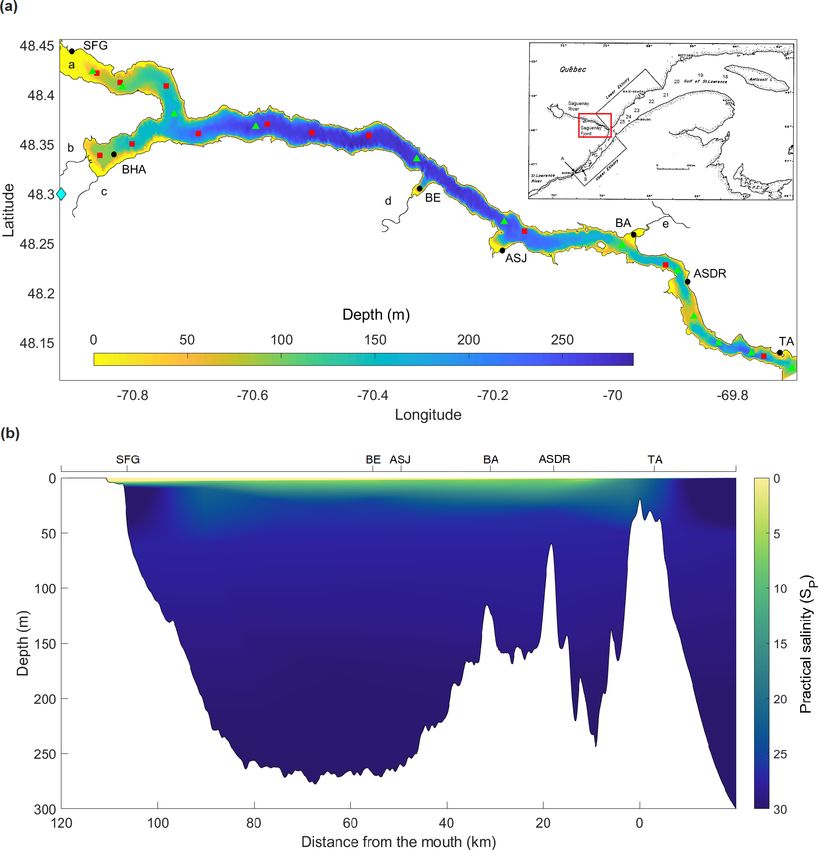
548                                              L. Delaigue et al.: Spatial variations in CO2 fluxes in the Saguenay Fjord

climate change on future fluxes are intricate given the very     al., 2012). Fjords stand amongst the most productive ecosys-
large uncertainty associated with present-day air–sea CO2        tems on the planet, while they have a yet unexplored role
flux estimates in coastal waters, including rivers, estuaries,   in regional and global carbon cycles as part of the estuarine
tidal wetlands and the continental shelf (Bauer et al., 2013;    family (Juul-Pedersen et al., 2015). They are crucial hotspots
Najjar et al., 2018). The coastal ocean occupies only ∼ 7 %      for organic carbon (mostly terrestrial) burial and account for
of the global ocean surface area but plays a major role in       nearly 11 % of the annual organic carbon burial flux in ma-
biogeochemical cycles because it (1) receives massive inputs     rine sediments, while covering only 0.12 % of oceans’ sur-
of terrestrial organic matter and nutrients through continen-    face (Rysgaard et al., 2012; Smith et al., 2015). In other
tal runoff and groundwater discharge; (2) exchanges matter       words, organic carbon burial rates in fjords are 100 times
and energy with the open ocean; and (3) is one of the most       faster than the average rate in the global ocean. Rates of or-
geochemically and biologically active areas of the biosphere,    ganic carbon burial provide insights into the mechanism that
accounting for significant fractions of marine primary pro-      controls atmospheric O2 and CO2 concentrations over geo-
duction (∼ 14 % to 30 %), organic matter burial (∼ 80 %),        logical timescales (Smith et al., 2015).
sedimentary mineralization (∼ 90 %), and calcium carbonate          This study presents (1) the relative contribution of known
deposition (∼ 50 %) (Gattuso et al., 1998).                      source waters to the water column in the Saguenay Fjord,
   Although the carbon cycle of the coastal ocean is acknowl-    estimated from the solution of an optimization multiparam-
edged to be a major component of the global carbon cy-           eter algorithm (OMP) using geochemical and isotopic trac-
cle and budget, accurate quantification of organic and inor-     ers, and (2) results of a conservative mixing model, based on
ganic carbon cycling and fluxes in the coastal ocean – where     results of the OMP analysis, and from which theoretical sur-
land, ocean and atmosphere interact – remains challenging        face water pCO2 values are derived and then compared to
(Bauer et al., 2013; Najjar et al., 2018). Constraining the      field measurements. The latter comparison serves to identify
exchanges and fates of different forms of carbon along the       the dominant factors, other than physical mixing (i.e., bio-
land–ocean continuum is so far incomplete, owing to lim-         logical activity, gas exchange), that impact the CO2 fluxes at
ited data coverage and large physical and biogeochemical         the air–sea interface and modulate their direction and inten-
variability within and between coastal subsystems (e.g., hy-     sity throughout the fjord (i.e., whether it is a source or a sink
drological and geomorphological differences, differences in      of CO2 to the atmosphere).
the magnitude and stoichiometry of organic matter inputs).
Hence, owing to limited data coverage and suspicious upscal-
ing due to the large physical and biogeochemical variability     2     Data and methods
within and between coastal subsystems, there remains a de-
bate as to whether coastal waters are net sources or sinks of    2.1    Study site characteristics
atmospheric CO2 . Recent compilations of worldwide CO2
partial pressure (pCO2 ) measurements indicate that most         Located in the subarctic region of Quebec, eastern Canada,
open shelves in temperate and high latitudes are sinks of at-    the Saguenay Fjord is up to 275 m deep, 110 km long and has
mospheric CO2 , whereas low-latitude shelves and most estu-      an average width of 2 km, with a 1.1 km wide mouth where
aries are sources (Chen and Borges, 2009; Cai, 2011; Chen        it connects to the head of the Lower St. Lawrence Estuary
et al., 2013). As noted by Bauer et al. (2013), estuaries are    (Fig. 1a). The fjord’s bathymetry includes three basins bound
transitional aquatic environments that can be riverine or ma-    by three sills (Fig. 1b). The first one, at a depth of ∼ 20 m, is
rine dominated and, thus, they typically display strong gradi-   located at its mouth near Tadoussac and controls the overall
ents in biogeochemical properties and processes as they flow     dynamics of the fjord. The second is located 18 km further
seaward. Chen et al. (2013) reported that the strength of es-    upstream and sits at a depth of 60 m, while the third one is
tuarine sources typically decreases with increasing salinity.    found another 32 km further upstream and rises to a depth of
However, marsh-dominated estuaries, in which active micro-       115 m. The fjord’s drainage basin is 78 000 km2 and is part of
bial decomposition of organic matter occurs in the intertidal    the greater St. Lawrence drainage basin (Smith and Walton,
zone, are strong sources of CO2 (Cai, 2011).                     1980), forming a hydrographic system, along with the Great
   High-latitude waters such as the Arctic Ocean have re-        Lakes, of more than 1.36 million km2 .
cently been the foci of much research, while coastal, season-       Tributaries to the Saguenay Fjord include the Saguenay,
ally ice-covered aquatic environments, such as the Saguenay      Éternité and Sainte-Marguerite rivers (Fig. 1a). The Sague-
Fjord, that display comparable inter-annual and climatic sea-    nay River is the main outlet from Saint-Jean Lake and flows
ice cover variabilities but are much more accessible, have       into the north arm of the fjord near St. Fulgence (Fig. 1a) with
been neglected (Bourgault et al., 2012). Characteristics of      a mean freshwater discharge of ∼ 1200 m3 s−1 (Bélanger,
Arctic coastal ecosystems are found in the Saguenay Fjord,       2003). Two other local, minor tributaries, the Rivière-à-Mars
including the presence of many species of plankton, fish,        (95 km long, mean discharge ∼ 8 m3 s−1 ) and the Rivière
birds and marine mammals, as well as important freshwater        des Ha! Ha! (35 km long, mean discharge ∼ 15 m3 s−1 ) dis-
inputs and the presence of seasonal ice cover (Bourgault et      charge into the Baie des Ha! Ha!, a distinct feature of the

Biogeosciences, 17, 547–566, 2020                                                      www.biogeosciences.net/17/547/2020/
L. Delaigue et al.: Spatial variations in CO2 fluxes in the Saguenay Fjord                                                             549

Figure 1. (a) Bathymetry and geographic location of the Saguenay Fjord. Red squares represent the hydrographic stations sampled during
R/V Coriolis II cruises in September 2014, May 2016, June 2017 and May 2018. Green triangles represent the hydrographic stations sampled
during a SECO.net cruise onboard the R/V Coriolis II in November 2017. The approximate locations of the following are shown: Tadoussac
(TA), L’Anse de Roche (ASDR), Baie Sainte-Marguerite (BA), Anse-Saint-Jean (ASJ), Baie-Eternité (BE), St. Fulgence (SFG), Baie des
Ha! Ha! (BHA). The main tributaries to the fjord are also shown, including the Saguenay River (a), Rivière-à-Mars (b), Rivière des Ha! Ha!
(c), Éternité River (d) and Sainte-Marguerite River (e). The blue diamond identifies the location of the La Baie weather station. Letters (A
to K) and numbers (18 to 25) in the inset indicate the location of sampling stations in the St. Lawrence Estuary where data were acquired to
define the SLRW, LSLE and CIL end-members. (b) Longitudinal section along the Saguenay Fjord, showing the strong halocline.

Saguenay Fjord (Fig. 1a). Finally, the fjord receives denser               The overflow and the intrusion of marine waters from the
marine waters from the St. Lawrence Estuary, filling the bot-           St. Lawrence Estuary generate a sharp halocline, leading to
tom of the three basins, as these waters episodically over-             a simplified two-layer stratification in the fjord (Fig. 1b).
flow the entrance sill (Therriault and Lacroix, 1975; Stacey            The tidally modulated intrusion of marine waters from the
and Gratton, 2001; Bélanger, 2003; Belzile et al., 2016). Ac-           St. Lawrence Estuary into the Saguenay Fjord, as well as
cording to Seibert et al. (1979), the tidal amplitude at the            the outflow of the fjord into the estuary, have a major influ-
mouth of the fjord near Tadoussac averages 4.0 m and in-                ence on the water column stratification and circulation in the
creases slightly toward the head of the fjord (4.3 m near Port          Saguenay Fjord and at its mouth (Belzile et al., 2016; Mucci
Alfred). Spring tides may reach an amplitude of 6 m.                    et al., 2017). In other words, the properties of the uppermost
                                                                        100 m of the water column in the adjacent estuary are critical

www.biogeosciences.net/17/547/2020/                                                                 Biogeosciences, 17, 547–566, 2020
550 L. Delaigue et al.: Spatial variations in CO2 fluxes in the Saguenay Fjord
in determining the water stratification in the Saguenay Fjord, Dubuc Bridge that joins Chicoutimi and Chicoutimi-Nord,
since salinity and temperature control the density of waters to determine the chemical characteristics of the freshwater
that spill over the sill and fill the fjord’s deep basins (Belzile Saguenay River end-member.
et al., 2016). The rosette system (12 × 12 L Niskin bottles) was
During most of the ice-free season, the St. Lawrence Es- equipped with a Seabird 911Plus conductivity–temperature–
tuary is characterized by three distinct layers: (1) a rela- depth (CTD) probe, a Seabird® SEB-43 oxygen probe, a
tively warm and salty bottom layer (LSLE, 4 ◦ C < T < 6 ◦ C, WETLabs® C-Star transmissometer and a Seapoint® fluo-
34 < SP < 34.6, where T stands for temperature and SP refers rometer. The Niskin bottles were closed at discrete depths
to practical salinity) that originates from mixing on the con- as the rosette was raised from the bottom, typically at the
tinental shelf of Northwestern Atlantic Current and Labrador surface (2–3 m), 25, 50, 75, 100 and at 50 m intervals to the
Current waters, (2) a cold intermediate layer (CIL, 30– bottom (or within 10 m of the bottom). Samples were taken
150 m deep; −1 ◦ C < T < 2 ◦ C, 31.5 < SP < 33) that forms in directly from the bottles for dissolved oxygen (DO), pHNBS
the Gulf of St. Lawrence in the winter and flows land- and/or pHT , total alkalinity (TA), dissolved inorganic car-
ward, and (3) a warm brackish surface layer (0–30 m deep, bon (DIC), dissolved silicate (DSi), practical salinity (SP ),
−0.6 ◦ C < T < 12 ◦ C, 25 < SP < 32) that results from the mix- and the stable oxygen isotopic composition of the water
ture of freshwater from various tributaries (mostly the St. (δ 18 Owater ). Water samples destined for pH measurements
Lawrence and Saguenay rivers but also north-shore rivers were transferred to 125 mL plastic bottles without headspace,
such as the Betsiamites, Romaine and Manicouagan) and whereas TA and TA/DIC samples were stored in, respec-
seawater and flows seaward to ultimately form the Gaspé tively, 250 and 500 mL glass bottles. TA and TA/DIC sam-
Current (Dickie and Trites, 1983; El-Sabh and Silverberg, ples were poisoned with a few crystals of mercuric chloride
1990; Gilbert and Pettigrew, 1997). Seasonal variations (HgCl2 ), and bottles were sealed using a ground-glass stop-
greatly affect the properties of the surface layer, which per and Apiezon® Type-M high-vacuum grease. δ 18 Owater
merges with the intermediate layer during winter, as temper- and SP samples were stored in 13 mL plastic screw-cap test
ature and salinity change with atmospheric, and buoyancy tubes.
forcing and the contribution from tributaries decreases dur- Direct measurements of surface water (∼ 2 m) pCO2 were
ing winter months (Galbraith, 2006). carried out using a CO2 -Pro CV (Pro-Oceanus, Bridgewa-
Likewise, the Saguenay Fjord is characterized by a ter, NS) probe in May 2018. The CO2 -Pro CV probe op-
strongly stratified water column that includes at least two erates through rapid diffusion of gases through a supported
water masses: (1) a warm, shallow layer, the Saguenay semipermeable membrane to a thermostated cell in which the
Shallow Water (SSW; 0 ◦ C < T < 16.8 ◦ C, 0.2 < SP < 26.9), CO2 mole fraction is quantified by a nondispersive infrared
that lies above (2) the Saguenay Deep Water (SDW; detector (NDIR) that was factory calibrated using standard
0.9 ◦ C < T < 4.0 ◦ C, 27.3 < SP < 29.8). The SDW most likely trace gas mixtures. The instrument was operated in continu-
forms from a mixture of surface fjord water, St. Lawrence ous mode, with measurements taken nearly every 7 s. Stable
River waters and the St. Lawrence Estuary cold intermedi- pCO2 values were achieved after a 15 min equilibration pe-
ate layer (CIL), when the latter spills over the entrance sill riod and averaged over the next 20 min. Relative standard de-
at the mouth of the fjord (Bourgault et al., 2012; Belzile et viations over this period were typically on the order of 0.2 to
al., 2016). Nonetheless, our study shows that, because the 6 % but were on the order of 0.1 % in a stable water mass at
Saguenay Fjord is a relatively deep fjord with multiple sills, 220 m depth, implying that deviations recorded at the surface
the vertical structure of the water column is far more complex likely reflected natural variations over the period of sampling
than described above. as the ship drifted with the current. The manufacturer claims
a 1 % accuracy, but the performance of the instrument may
2.2 Water column sampling be even better (Hunt et al., 2017).
Total freshwater discharge data of the Saguenay River
The data presented in this paper were gathered on five were provided by Rio Tinto Alcan (a multinational alu-
cruises, between the years 2014 and 2018 aboard the R/V minum smelter and producer that manages its own hydro-
Coriolis II in late spring (May 2016 and May 2018) and early electric dam on the Saguenay River) from their bank sta-
summer (June 2017), as well as early and late fall (Septem- bilization program. Data for the relevant sampling days in
ber 2014 and November 2017). Sampling of the water col- September 2014, May 2016, June 2017, November 2017 and
umn was carried out with a rosette system along the cen- May 2018 were taken from the Shipshaw and Chute-à-Caron
tral axis of the Saguenay Fjord, between St. Fulgence and monitoring stations.
the mouth of the fjord, including the Baie des Ha! Ha!. Sta-
tions in the St. Lawrence Estuary, near the mouth of the fjord, 2.3 Analytical procedures
were also sampled. The sampling locations are identified in
Fig. 1a. The surface water of the Saguenay River was sam- T and SP were determined in situ using the CTD probe. The
pled, with a rope and bucket in 2013 and 2017, from the conductivity probe was calibrated by the manufacturer over
Biogeosciences, 17, 547–566, 2020 www.biogeosciences.net/17/547/2020/L. Delaigue et al.: Spatial variations in CO2 fluxes in the Saguenay Fjord 551
the winter prior to the cruises. In addition, the SP of sur- waters were transferred into 3 mL vials stoppered with a
face waters was determined by potentiometric argentometric septum cap. The vials were then placed in a heated rack
titration at McGill University and calibration of the AgNO3 maintained at 40 ◦ C. Commercially available 99.998 % pure
titrant with IAPSO standard seawater. The reproducibility of CO2 gas (Research Grade) was introduced in all the vials
these measurements is typically better than ±0.5 %. using a Micromass AquaPrep and allowed to equilibrate
pHT was determined spectrophotometrically on board, on for 7 h. The headspace CO2 was then sampled by the Mi-
the total hydrogen ion concentration scale for saline wa- cromass AquaPrep, dried on a −80 ◦ C water trap and an-
ters (SP > 5), using phenol red and purified m-cresol purple alyzed on a Micromass Isoprime universal triple collector
as indicators and a Hewlett-Packard UV-visible diode array isotope ratio mass spectrometer in dual inlet mode at the
spectrophotometer (HP-8453A) with a 5 cm quartz cell, af- GEOTOP-UQAM Stable Isotope Laboratory. Data were nor-
ter thermal equilibration of the sample in a constant tem- malized against the three internal reference waters, them-
perature bath at 25 ◦ C ±0.1. The salinity-dependence of the selves calibrated against Vienna Standard Mean Ocean Water
dissociation constants and molar absorptivities of the indica- (V-SMOW) and Vienna Standard Light Arctic Precipitation
tors were taken from Robert-Baldo et al. (1985) for phenol (V-SLAP). The results are reported on the δ scale in ‰ rela-
red and from Clayton and Byrne (1993) for m-cresol purple. tive to V-SMOW:
The salinity-dependence of the phenol red indicator dissoci- !
ation constant and molar absorptivities was extended (from 18 (18 O/16 O)sample
δ O= − 1 × 1000. (1)
SP = 5 to 35; Bellis, 2002) to encompass the range of salini- (18 O/16 O)standard
ties encountered in this study, but computed pHT values from
the revised fit were not significantly different from those Based on replicate analyses of the samples, the average stan-
obtained with the relationship provided by Robert-Baldo et dard deviation of the measurements was better than 0.05 ‰.
al. (1985). Results computed from these parameters yielded TA was measured using an automated Radiometer
values that were more similar to each other as well as to po- (TitraLab865® ) potentiometric titrator and a Red Rod® com-
tentiometric glass electrode measurements than the revised bination pH electrode (pHC2001) at McGill University. The
equation for the purified m-cresol purple provided by Dou- diluted HCl titrant was calibrated prior, during and af-
glas and Byrne (2017). The pH of low-salinity waters (SP < 5) ter each titration session using certified reference materials
was determined potentiometrically on board at 25 ◦ C, on (CRMs) provided by Andrew Dickson (Scripps Institution
the NIST (formerly NBS) scale (pHNBS ), using a Radiome- of Oceanography). Raw titration data were processed with a
ter Analytical® (GK2401C) combination glass electrode proprietary algorithm designed for shallow endpoint detec-
connected to a Radiometer Analytical® pH/millivoltmeter tion. Surface water samples from the Saguenay Fjord and the
(PHM84). A calibration of the electrode was completed Upper St. Lawrence Estuary were also analyzed at Dalhousie
prior to and after each measurement, using three NIST- University using a VINDTA 3C® (Versatile Instrument for
traceable buffer solutions: pH 4.00, pH 7.00 and pH 10.00 the Determination of Titration Alkalinity, by Marianda) fol-
at 25 ◦ C. The Nernstian slope was then obtained from the lowing the method described in Dickson et al. (2007). A
least-squares fit of the electrode response to the NIST buffer calibration of the instrument was performed against CRMs,
values. For waters with SP of between 5 and 35, pHNBS and the reproducibility of the measurements was better than
was converted to pHT according to the electrode response to 0.1 %.
TRIS (tris(hydroxymethyl)aminomethane) buffer solutions The DIC concentration of samples, recovered in 2016,
prepared at SP = 5, 15, 25 and 35 and for which the pHT 2017 and 2018 in the Saguenay Fjord and surface waters of
was assigned at 25 ◦ C (Millero, 1986). Reproducibility of pH the Upper and Lower St. Lawrence Estuary, were determined
measurements based on replicate analyses of the same sam- at Dalhousie University using the VINDTA 3C® . In 2014,
ple or at least two of the three methods used was typically DIC was determined on board using a SciTech Apollo DIC
better than ±0.005. analyzer. Once thermally equilibrated at 25 ◦ C, 1–1.5 mL of
Dissolved oxygen (DO) concentrations were determined the sample was acidified with 10 % H3 PO4 after being in-
on board by Winkler titration on distinct water samples jected into the instrument’s reactor. The evolved CO2 was
recovered directly from the Niskin bottles, following the carried to a LI-COR infrared analyzer by a stream of pure
method described by Grasshoff et al. (1999). The relative nitrogen. A calibration curve was constructed using gravi-
standard deviation, based on replicate analyses of samples metrically prepared Na2 CO3 solutions, and the accuracy of
recovered from the same Niskin bottle, was 0.5 %. These the measurements was verified using a CRM. Reproducibil-
measurements served to calibrate the SBE-43 oxygen probe ity was typically on the order of 0.2 %.
mounted on the rosette sampler.
The stable oxygen isotopic composition of the water sam-
ples (δ 18 Owater ) was determined using the CO2 equilibration
method of Epstein and Mayeda (1953). Aliquots (200 µL)
of the water samples and three laboratory internal reference
www.biogeosciences.net/17/547/2020/ Biogeosciences, 17, 547–566, 2020552 L. Delaigue et al.: Spatial variations in CO2 fluxes in the Saguenay Fjord
2.4 Calculations dure based on covariances between tracers is typically ap-
plied. In this study, weights were assigned arbitrarily based
2.4.1 Water mass distribution analysis on their conservative behaviors and variability (Lansard et
al., 2012). Conservative tracers (i.e., SP , TA, δ 18 Owater ) were
A combination of transport processes associated with ocean assigned heavy weights, while nonconservative tracers (i.e.,
circulation and biogeochemical cycles generally controls the T , DO, DIC) were given low weights according to their sea-
distribution of tracers in the ocean (Chester, 1990). Resolv- sonal variability. For instance, temperatures in the surface
ing the effects of mixing and biogeochemical cycling is im- waters of the Saguenay River range from 3.1 ◦ C in the winter
perative if one is to evaluate the movement of nutrients and to 21 ◦ C in the summer. Dissolved oxygen was also consid-
tracers in a water body. An optimum multiparameter (OMP) ered a nonconservative tracer as it is heavily reliant on tem-
analysis allows for the determination of the relative contribu- perature and salinity, as well as biological activity. DIC was
tions of pre-defined source water types (SWTs), represent- given an intermediate weight given that it is relatively con-
ing the parameter values of the unmixed water masses in servative except in the surface waters, where photosynthesis
one specific geographic location, by optimizing the hydro- and air–sea gas exchange take place. Several OMP analy-
graphic data gathered in a given system (Tomczak, 1981). ses were carried out using different weights for each parame-
The original OMP algorithm is a linear inverse model that ter, while weighing their conservative behavior appropriately
assumes all hydrographic tracers are conservative. The al- (i.e., highly conservative vs. lightly conservative). Results
gorithm has since been modified to handle nonconservative were not affected significantly.
properties such as DIC and nutrients by taking into consid-
eration the stoichiometry of microbial respiration and photo- 2.4.2 Source water type definitions
synthesis (Dinauer and Mucci, 2018; Karstensen and Tom-
czak, 1998). A water mass is, by definition, a body of water having its ori-
OMP calculates the SWT fractions, xi , for each data point gin in a particular source region (Tomczak, 1999). An OMP
by finding the best linear mixing combination defined by pa- analysis requires the user to define the major water masses
rameters such as T , SP , δ 18 Owater , DO, TA and DIC. The contributing to the structure of the water column in the study
contributions from all SWT must add up to 100 % and can- area. In the context of biogeochemical cycles, a SWT should
not be negative. Assuming that four SWT (a, b, c and d) are be defined where the water mass enters the basin, before it
sufficient to characterize the water column structure, and six enters the mixing region (Karstensen, 2013). Parameter val-
parameters (T , S, δ 18 Owater , DO, TA and DIC) characterize ues are preferably extrapolated from hydrographic observa-
each of these, the following set of linear equations is solved tions in the water mass formation region or can be found in
in the classical OMP analysis (MATLAB – version 1.2.0.0; the literature.
Karstensen, 2013): In this study, source water type definitions were derived
from property–property diagrams (see Appendix, Fig. A1) of
xa Ta + xb Tb + xc Tc + xd Td = Tobs + RT , (2a) an observational dataset relevant to the Saguenay Fjord: the
xa Sa + xb Sb + xc Sc + xd Sd = Sobs + RS , (2b) Saguenay River (SRW), the St. Lawrence Estuary summer-
18 18 18 18 time cold intermediate layer (CIL), the Lower St. Lawrence
xa δ Oa + xb δ Ob + xc δ Oc + xd δ Od
Estuary bottom waters (LSLE) and the St. Lawrence River
= δ 18 Oobs + Rδ 18 O , (2c) (SLRW). Each definition was captured relative to the fjord,
xa DOa + xb DOb + xc DOc + xd DOd = DOobs + RDO , (2d) i.e., each source water type is only appropriate for the fjord
and for the period of study. Definitions and weights are re-
xa TAa + xb TAb + xc TAc + xd TAd = TAobs + RTA , (2e)
ported in Table 1. A seasonality analysis was carried out to
xa DICa + xb DICb + xc DICc + xd DICd ensure SWT definitions were appropriate for the period of
= DICobs + RDIC , (2f) study. Insignificant variations were observed in tracers such
xa + xb + xc + xd = 1 + RP , (2g) as δ 18 O, DIC, TA, DO and SP . The only highly variable tracer
was T , which was given the lowest possible weight in the
where Tobs , Sobs , δ 18 Oobs , DOobs , TAobs and DICobs are the OMP analysis.
observed values in any given parcel of water and R is their
respective associated fitting residual. Ti , Si , δ 18 Oi , DOi ,
TAi and DICi (i = a, . . . , d) are the characteristic values
of each SWT (Lansard et al., 2012; Tomczak and Large,
1989; Mackas et al., 1987). Mass conservation is expressed
in Eq. (2g).
To account for potential environmental variability and
measurement inaccuracies and allow for the comparison of
parameters with incommensurable units, a weighting proce-
Biogeosciences, 17, 547–566, 2020 www.biogeosciences.net/17/547/2020/L. Delaigue et al.: Spatial variations in CO2 fluxes in the Saguenay Fjord 553
Table 1. Source water type (SWT) definitions for the Saguenay River (SRW), the St. Lawrence Estuary summertime cold intermediate layer
(CIL), the Lower St. Lawrence Estuary bottom water (LSLE) and the St. Lawrence River (SLRW). Definitions and variances were derived
from data taken in September 2014, May 2016, June 2017 and November 2017. Data for SRW and SLRW were extrapolated to SP = 0. The
weights used in the OMP analysis are also shown.
SWT Salinity Temperature (◦ C) TA(meas) (µmol kg−1 ) δ 18 O (‰) DIC (µmol kg−1 ) DO (µmol L−1 )
SRW 0.00 ± 0 6.19 ± 0.18 154 ± 13 −12.17 ± 0.21 230 ± 12 411 ± 6
CIL 32.52 ± 0.05 1.44 ± 0.08 2210 ± 2 −1.12 ± 0.03 2141 ± 3 256 ± 5
LSLE 34.31 ± 0.01 5.16 ± 0.18 2294 ± 2 −0.17 ± 0.02 2276 ± 3 76 ± 1
SLRW 0.00 ± 0 12.11 ± 0.13 1099 ± 16 −8.09 ± 0.13 1140 ± 15 329 ± 5
Weights 25 1 25 25 15 1
Table 2. Mean standard error of the mean and range of pCO2(SW) , k, u and F in the Saguenay Fjord surface waters. Numbers in parentheses
indicate the observed or calculated ranges. Overall, the total area-averaged degassing flux of the fjord adds up to 2.14 ± 0.43 mmol m−2 d−1
or 0.78 ± 0.16 mol m−2 yr−1 .
Sampling month pCO2(SW-calc) (µatm) k (cm h−1 ) u (m s−1 ) F (mmol m−2 d−1 )
May 2018 623 ± 26 1.94 ± 0.01 3.91 6.2 ± 0.79
(511/740) (1.89/1.97) (2.9/10.0)
November 2017 418 ± 12 3.2 ± 0.04 4.2 0.40 ± 0.51
(353/530) (2.82/3.38) (−2.4/4.8)
June 2017 506 ± 35 0.37 ± 0.01 1.89 0.42 ± 0.15
(315/663) (0.36/0.42) (−0.4/1.1)
May 2016 563 ± 31 1.26 ± 0.01 3.17 3.04 ± 0.62
(349/724) (1.15/1.30) (−1.1/6.5)
September 2014 406 ± 6 1.43 ± 0.01 3.71 0.16 ± 0.10
(369/432) (1.39/1.49) (−0.43/0.56)
2.4.3 CO2 partial pressures organic alkalinity (positive organic acidity) (see below). The
carbonic acid dissociation constants (K1∗ and K2∗ ) of Cai and
Wang (1998) were used for the calculations, as the latter were
The CO2 partial pressure in seawater (pCO2(SW) ) is defined found to be more suitable for the low-salinity waters encoun-
as the pCO2 in water-saturated air (pCO2(air) ) in equilib- tered in estuarine environments, such as the Saguenay Fjord
rium with the water sample or the ratio of the CO2 concen- (SP < 20) (Dinauer and Mucci, 2017). pCO2(SW-calc) values
tration in solution to the equilibrium concentration at T , P , were computed for the surface mixed layer located above the
and SP , multiplied by the actual pCO2(air) . As direct mea- sharp pycnocline (∼ 10 m), where most physical and chem-
surements of the surface mixed layer pCO2 were not avail- ical properties are directly impacted by biological activity
able in September 2014, May 2016, June 2017 and Novem- (photosynthesis and respiration), as well as heat and gas ex-
ber 2017, it was calculated (pCO2(SW-calc) ) using CO2SYS change across the air–sea interface (Table 2). Direct measure-
(Excel v2.1; Pierrot et al., 2006) and the measured pH (to- ments of pCO2 (pCO2(SW-meas) ) were acquired in May 2018,
tal or NBS/NIST scale; see Appendix B, Tables B1 and B2), and pCO2(SW-calc) was also calculated from pH and DIC for
DIC (µ mol kg−1 ), in situ temperature ( ◦ C), practical salinity this sampling month for comparison purposes, following the
(SP ) and pressure (dbar) as input parameters. When avail- aforementioned procedure.
able, soluble reactive phosphate (SRP) and dissolved silicate
(DSi) concentrations were also included in the calculations,
but their inclusion did not affect the results significantly be- 2.4.4 CO2 flux across the air–sea interface
cause their concentrations are relatively low in surface waters
(0.49 and 37.0 µM, respectively) and introduce an insignifi- The difference between the air and sea surface pCO2 values
cant error. DIC rather than TA was used as an input param- (1pCO2 = pCO2(SW) – pCO2(air) ) determines the direction
eter to CO2SYS, since the fjord surface waters are enriched of gas exchange and whether the surface mixed layer of a
in colored dissolved organic carbon (> 4 mg L−1 ) delivered body of water is a source or a sink of CO2 for the atmosphere.
by the Saguenay River and are characterized by a negative The air–sea CO2 gas exchange, or CO2 flux, can be estimated
www.biogeosciences.net/17/547/2020/ Biogeosciences, 17, 547–566, 2020554 L. Delaigue et al.: Spatial variations in CO2 fluxes in the Saguenay Fjord
at each station using the following relationship: and Climate Change Canada. The mean pCO2(air) was then
calculated for each year using the following equation:
FCO2 = k · K0 · (1pCO2 ), (3a)
pCO2(air) = xCO2 · (Pb − Pw ), (4)
where F is the flux of CO2 across the air–sea interface
in mmol m−2 d−1 , k is the gas transfer velocity of CO2 in
where xCO2 is the measured mole fraction of CO2 in dry
cm h−1 (Wanninkhof, 1992), K0 is the solubility of CO2 in
air in ppm, Pb is the barometric pressure at the sea surface
mol kg−1 atm−1 at the in situ temperature and salinity of
in atm, and Pw is the saturation water vapor pressure at in
the surface waters (Weiss, 1974), and 1pCO2 is the differ-
situ temperature and salinity in atm. Pb was obtained using
ence between the air and sea surface pCO2 values in µatm.
the conversion formula of Tim Brice and Todd Hall (from
Whereas, formally, Fick’s first law of diffusion should be
NOAA’s National Weather Service – https://www.weather.
written as F = −D δC/δx (where F is the diffusion flux in
gov/epz/wxcalc_wxcalc2go, last access: 3 November 2019),
mole s−1 m−2 , D is the diffusion coefficient in m2 s−1 , C is
using the La Baie weather station’s elevation (152 m). Pw
the concentration of CO2 in mole m−3 and x is the distance
was calculated using the Rivière-à-Mars properties (i.e., clos-
in m), as commonly expressed by Eq. (3a), positive values
est body of water to the weather station), and the Pw calcu-
of F indicate the release of CO2 to the atmosphere by sur-
lated from its relationship to T and SP provided by Weiss and
face waters, whereas negative values imply that surface wa-
Price (1980).
ters serve as a sink of atmospheric CO2 . The flux of CO2 was
The area-averaged CO2 flux (Farea-avg ) was computed for
computed for each sampling month, using the pCO2(air) for
the whole fjord, following the procedure described by Jiang
each sampling date (395 µatm for September 2014, 407 µatm
et al. (2008):
for May 2016, 408 µatm for June and November 2017, and
411 µatm for May 2018; see below for details). 6Fi × Si
The gas transfer velocity of CO2 was calculated using the Farea−avg = , (5)
6 Si
revised relationship of Wanninkhof (2014):
where Fi is the average of all the fluxes within segment i and
k = 0.215u2 (Sc/660)−1/2 , (3b) Si is the surface area of segment i. The fjord was divided into
where u is the wind speed (m s−1 ) and Sc is the Schmidt two segments, one including the inner basin and the other en-
number (Wanninkhof, 2014). Wind speed was estimated us- compassing the two outer basins, as each segment often dis-
ing the hourly station wind speed data from Environment plays distinct behaviors. Segments are identified in Fig. 1b.
Canada at the La Baie weather station (Fig. 1a) for each The fjord’s surface area (∼ 290 km2 ) was computed using a
sampling month. The Schmidt number is defined as the kine- land mask in MATLAB.
matic viscosity of water divided by the diffusion coefficient
2.4.5 Water mixing model
of CO2 . Sc was corrected for the temperature dependence of
CO2 in freshwater (SP = 0), assuming that k is proportional A two end-member mixing model was constructed based on
to Sc−1/2 (Wanninkhof, 1992). In the case of CO2 , the in- the chemical properties of the freshwater delivered to the
crease in Sc−1/2 (and k) with increasing temperature is com- fjord (Saguenay River) and marine bottom waters entering
pensated for by a decrease in solubility; therefore, k was con- the fjord from the St. Lawrence Estuary (Fig. 2a). As shown
sidered nearly temperature independent (Wanninkhof, 1992). in the results of the OMP analysis (Sect. 3.1), the LSLE and
Sc was computed using the following equation: SLRW have a negligible influence on the fjord’s water struc-
Sc = +Bt + Ct 2 + Dt 3 + Et 4 , (3c) ture and thus were not included in the model. Given that the
carbonate chemistries of the CIL and LSLE waters are sim-
where t is the temperature (◦ C) and A, B, C, D, and E are fit- ilar, the bottom waters were assumed to be well mixed and
ting coefficients for seawater (SP = 35) and freshwater (SP = constitute a single end-member. This is illustrated in Fig. 2,
0), for water temperatures ranging from −2 to 40 ◦ C (Wan- as the high SP end-member alkalinity extends linearly be-
ninkhof, 2014). The uncertainty in Sc ranges from 3 % to yond that of the CIL end-member (Table 1). The measured
10 % and is mainly due to the imprecision of diffusion coeffi- surface TAs were strongly correlated to SP (R 2 = 0.999) in
cients (Wanninkhof, 2014). Estimates of k, calculated at each the fjord waters. Therefore, end-member properties were ob-
sampling point using the equation of Wanninkhof (2014), tained by extrapolating the surface water (above the pycn-
ranged from 0.36 to 3.38 cm h−1 for the fjord, compared to ocline) data to SP = 0 and bottom water data to the high-
1.6 to 4.5 cm h−1 in the St. Lawrence Estuary (Dinauer and est measured salinity (Fig. 2a). The extrapolated TA(meas)
Mucci, 2017). (Fig. 2b; 154 µmol kg−1 ) is in good agreement with the av-
Atmospheric pCO2 values (pCO2(air) ) were computed us- erage TA(meas) of samples taken directly from the Saguenay
ing the daily averages of measured mole fractions of CO2 River in 2013 and 2017 (157 µmol kg−1 ). The organic alka-
in dry air, obtained at the La Baie weather station and re- linity of the fjord waters was estimated from the difference
trieved from the Climate Research Division at Environment between the measured and calculated TA (TA(calc) ; Fig. 2b).
Biogeosciences, 17, 547–566, 2020 www.biogeosciences.net/17/547/2020/L. Delaigue et al.: Spatial variations in CO2 fluxes in the Saguenay Fjord 555
higher salinities, the pCO2(SW-mix) is elevated and the fjord
serves as a net source of CO2 to the atmosphere, but at in-
termediate salinities (5 < SP < 15) or mixing ratios, the fjord
may serve as a net sink of atmospheric CO2 when surface
water temperatures are close to freezing. The data from the
various cruises are superimposed on the model results, after
correction for the organic alkalinity.
2.4.6 Salinity normalization of DIC in surface waters
To quantitatively evaluate the impact of biological activity
on the DIC budget in the surface waters of the fjord, DIC and
TA(calc) were normalized to the average surface salinity of
each sampling month (SP = 12.4 for September 2014; SP =
2.58 for May 2016; SP = 7.61 for June 2017; SP = 10.9 for
November 2017; and SP = 5.9 for May 2018) following the
procedure of Friis et al. (2003):
DICmeas − DICS=0 ref
NDIC = · S + DICS=0 , (7)
S meas
where DICmeas is the measured DIC, DICS=0 is the DIC ex-
trapolated to SP = 0, S meas is the measured practical salinity
and S ref is the average measured practical salinity per sam-
Figure 2. (a) Measured alkalinity (TA(meas) ) vs. practical salinity
pling month (Friis et al., 2003). The change in NDIC (i.e.,
(SP ) for SRW and CIL data points for all sampling months (R 2 =
1NDIC) along the fjord, relative to the waters at the head
0.999). The triangle defines the properties of the SRW, and the
of the fjord, was then computed for each sampling month.
square comprises the properties of the CIL. (b) TA(meas) , TA(calc)
and Org Alk definitions for the Saguenay River (SRW), using sur- These values reveal how DIC evolves along the fjord beyond
face water data from all sampling months, with standard error. The what is expected based on conservative mixing.
Org Alk (positive) contribution to the TA of the CIL is not consid-
ered, as it accounts for less than 0.1 % of its TA. 2.4.7 Oxygen saturation and apparent oxygen
utilization in the surface waters
The latter was calculated using CO2SYS (Excel v2.1; Pier- To further account for the biological activity in the surface
rot et al., 2006) and pH and DIC as input parameters. The waters, the oxygen saturation index was calculated for each
end-member source waters were then mixed, assuming that sampling month in the surface waters of the fjord using the
TA(calc) and DIC behave conservatively. Hence, the salin- following equation:
ity, total alkalinity (TA(mix) ) and dissolved inorganic carbon
(DIC(mix) ) of the mixed solutions were calculated using the
following equations: %sat = ([O2 ]meas /[O2 ]equil ) × 100, (8)
m1 SP1 + m2 SP2 where [O2 ]meas is the dissolved oxygen concentration mea-
SP(mix) = , (6a)
(m1 + m2 ) sured in the fjord waters and [O2 ]equil is the equilibrium dis-
m1 TA(calc)−1 + m2 TA(calc)−2 solved oxygen concentration (or solubility) at in situ condi-
TA(mix) = , (6b)
(m1 + m2 ) tions (i.e., temperature and salinity) for each sample.
m1 DIC1 + m2 DIC2 The oxygen saturation index indicates if the system is au-
DIC(mix) = , (6c) totrophic (i.e., production of oxygen, dominated by photo-
(m1 + m2 )
synthesis) or heterotrophic (consumption of oxygen, domi-
where mi is the mass contribution of each end-member to the nated by microbial respiration). The oxygen saturation re-
mixture. mains a qualitative proxy, as O2 exchange at the air–sea in-
pCO2(SW-mix) was then computed from TA(mix) and terface is about 9 times faster than CO2 exchange (Zeebe
DIC(mix) for practical salinities ranging from 0 to 33 at four and Wolf-Gladrow, 2001). The apparent oxygen utilization
different temperatures (0, 5, 10 and 15 ◦ C) using CO2SYS. (AOU) was also computed from the difference between
Results of the model (Fig. 8) show that, at the lower and [O2 ]equil and [O2 ]meas .
www.biogeosciences.net/17/547/2020/ Biogeosciences, 17, 547–566, 2020556 L. Delaigue et al.: Spatial variations in CO2 fluxes in the Saguenay Fjord
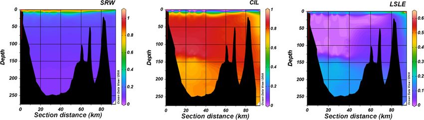
Figure 3. Vertical sections showing the relative contributions of the Saguenay River (SRW), the St. Lawrence Estuary cold intermediate layer
(CIL) and Lower St. Lawrence Estuary bottom waters (LSLE) to the water column structure of the Saguenay Fjord (June 2017). Fractions
were estimated using an optimum multiparameter (OMP) algorithm (Tomczak and Large, 1989; Tomczak, 1981; Mackas and Harrison,
1997). A variational analysis (DIVA) interpolation was applied between field data points in Ocean Data View.
3 Results and discussion counted, on average, for 2.2 % to 11.9 % of the total alka-
linity of the Saguenay River and varied annually and sea-
3.1 Water mass analysis sonally (−21 in September 2014, −39 in May 2016, −49
in June 2017, −22 in November 2017 and −18 µmol kg−1
Relative contributions (mixing ratios, f ) of the Saguenay in May 2018). It was inversely proportional to the salinity
River (SRW), the St. Lawrence Estuary summertime cold of the surface waters of the fjord and became positive, yet
intermediate layer (CIL) and Lower St. Lawrence Estuary a negligible fraction (< 0.1 %) of TA(corr) when SP > 25, like
(LSLE) bottom waters throughout the Saguenay Fjord’s wa- in the St. Lawrence Estuary. The negative organic alkalin-
ter column for the sampling month of June 2017 are shown in ity of the Saguenay River water most likely originates from
Fig. 3. As expected, the SRW and CIL are dominant contrib- soil humic acids that are flushed by percolation with ground-
utors, with the SRW forming a brackish surface layer (f = 1 waters that drain the metamorphic and igneous rocks of the
in surface waters) and the CIL replenishing the bottom wa- Canadian Shield. Surface water pCO2 (pCO2(SW-calc) ) values
ters of the fjord (0.7 < f < 1). According to the OMP anal- were higher at the head of the fjord (i.e., near the Saguenay
ysis, the LSLE bottom waters have a small contribution to River mouth) and lower at the mouth of the fjord, although
the fjord’s bottom waters (f = 0.2), adding to the complexity large variations (315 to 740 µatm – average 503 µatm) were
of the water structure. Although somewhat unexpected, this observed on a seasonal and yearly basis (Table 2). Values of
can readily be explained by tidal upwelling, internal waves pCO2(SW) were higher in May 2018 (623 µatm), June 2017
and intense turbulent mixing of the water column resulting (506 µatm), and May 2016 (563 µatm) than in November
from the rapid shoaling at the head of the Laurentian Channel 2017 (418 µatm) and September 2014 (406 µatm). This can
(Gratton et al., 1988; Saucier and Chassé, 2000). The relative be explained by the larger freshwater discharge from the
contribution of the LSLE bottom waters in the deep waters of Saguenay River in the spring (i.e., spring freshet, average
the fjord is small and could only be detected because of the of 1856 ± 21 m3 s−1 for spring periods of 1998–2018) com-
suite of geochemical and isotopic tracers used in the OMP pared to the fall (1470 ± 10 m3 s−1 for fall periods of 1998–
analysis, especially the difference in the δ 18 Owater signature 2018). As atmospheric pCO2(air) varied marginally between
of the CIL and LSLE waters. The contribution from the St. September 2014 (395 µatm) and May 2018 (411 µatm), the
Lawrence River Water (SLRW) is negligible, as it intrudes fjord was generally a source of CO2 to the atmosphere
slightly at the surface at the mouth of the fjord and is thus near its head (i.e., surface pCO2 values above atmospheric
not shown here. Although the water column structure is sim- level), while the zone near its mouth was most often a sink
ilar throughout the year, seasonal variations do occur and will (i.e., surface pCO2 values below atmospheric level) (Fig. 4).
be addressed in a forthcoming paper. An anomaly was observed in November 2017, with a high
pCO2(SW-calc) value (> 550 µatm) near the mouth of the fjord.
3.2 Aqueous pCO2 and CO2 flux Given the statistics of the box plot presented in Fig. 7, this
value appears to be erroneous.
Variations in the inorganic carbon chemistry in the Sague- Air–sea CO2 fluxes within the fjord ranged from −2.4
nay Fjord water column are described using field data ac- to 10.0 mmol m−2 d−1 (Fig. 6). Near the head of the fjord,
quired in September 2014, May 2016, June 2017, Novem- fluxes were mostly positive, while values decreased when
ber 2017 and May 2018. The organic alkalinity (acidity) ac-
Biogeosciences, 17, 547–566, 2020 www.biogeosciences.net/17/547/2020/L. Delaigue et al.: Spatial variations in CO2 fluxes in the Saguenay Fjord 557
ity (and buffer capacity) of the Saguenay River waters that
flow through the Grenvillian metamorphic and igneous rocks
of the Canadian Shield (Piper et al., 1990), as with most
rivers on the north shore of the St. Lawrence Estuary (e.g.,
Betsiamites, Manicouagan, Romaine; Paul del Giorgio, per-
sonal communication, 2016), and the low productivity of
the fjord surface waters because of very limited light pen-
etration due to their high chromotrophic dissolved organic
matter (CDOM) content (Tremblay and Gagné, 2009; Xie
et al., 2012). In contrast, waters of the St. Lawrence River
have an elevated carbonate alkalinity (∼ 1200 µM), inherited
from the Ottawa River that drains through limestone deposits
(Telmer and Veizer, 1999). Furthermore, the estuary is host
to multiple seasonal phytoplankton blooms (Levasseur and
Therriault, 1987; Zakardjian et al., 2000; Annane et al., 2015)
that strongly modulate its trophic status (Dinauer and Mucci,
2018).
The correlation between pCO2(SW-meas) and pCO2(SW-calc)
Figure 4. Spatial distribution of surface water pCO2(SW-calc) in is presented in Fig. 5. The average difference between
September 2014, May 2016, June 2017, November 2017 and May
pCO2(SW-meas) and pCO2(SW-calc) is 48 µatm, implying that
2018. Dashed lines represent the pCO2(air) in the sampling months
(respectively, 396 ppm in September 2014, 407 ppm in May 2016,
calculations underestimate pCO2(SW) values by approxi-
408 ppm in June and November 2017, and 411 ppm in May 2018). mately 7 % and thus contribute to the uncertainty associ-
Data points above the lines indicate that waters are sources of CO2 ated with CO2 fluxes. This discrepancy most likely origi-
to the atmosphere, whereas those below the lines identify waters nates from uncertainties associated with the carbonic acid
that are sinks of atmospheric CO2 . dissociation constants (K1∗ and K2∗ ) in low-salinity estuar-
ine environments, particularly those affected by strong or-
ganic alkalinities or acidities such as in the Saguenay Fjord
(Cai et al., 1998; Ko et al., 2016). This concurs with the re-
sults of Lueker et al. (2000), who showed that, depending
on the choice of K1∗ and K2∗ , computed pCO2(SW) values
from other carbonate system parameters (TA, DIC, pH) can
be up to 10 % lower than those of direct measurements. Con-
sequently, although the constants of Cai and Wang (1998)
are the most suitable for this study, direct measurements of
the pCO2(SW) should preferentially be carried out whenever
possible.
3.3 Water mixing model approach
As results of the OMP analysis reveal, LSLE and SLRW
have a negligible influence on the water properties in the
fjord, except for the latter near the mouth. Additionally, given
Figure 5. Correlation between pCO2(SW-meas) and pCO2(SW-calc) the relatively small contribution of the LSLE deep waters
for May 2018. The black line shows the linear regression with a and their similarity to the carbonate chemistry of the CIL,
null intercept (R 2 = 0.50). Error bars, in red, are smaller than the their influence is considered inconsequential on the prop-
symbol. erties of the mixture. Hence, a conservative mixing model
was constructed based on the chemical properties of the two
main source water masses in the fjord (i.e., SRW and the
approaching its mouth. Overall, the total area-averaged de- CIL mixture for bottom waters) and the relationship between
gassing flux of the fjord adds up to 2.14±0.43 mmol m−2 d−1 practical salinity and TA(corr) /DIC, respectively (Fig. 8).
or 0.78 ± 0.16 mol m−2 yr−1 . In comparison, the degassing pCO2(SW-calc) were normalized at each station to the aver-
flux in the adjacent St. Lawrence Estuary was estimated at age surface water temperature per sampling month (i.e., T =
between 0.36 and 0.74 mol m−2 yr−1 during the late spring 10.4 ◦ C for September 2014, T = 5.04 ◦ C for May 2016,
and early summer (Dinauer and Mucci, 2017). This dis- T = 11.9 ◦ C for June 2017, T = 7.13 ◦ C for November 2017
crepancy can be explained by the low carbonate alkalin- and T = 5.08 ◦ C for May 2018) to account for the effects
www.biogeosciences.net/17/547/2020/ Biogeosciences, 17, 547–566, 2020558 L. Delaigue et al.: Spatial variations in CO2 fluxes in the Saguenay Fjord Figure 6. (a) Spatial distribution of air–sea CO2 flux (mmol m−2 d−1 ) in the Saguenay Fjord for all cruises. Data points above the dashed line indicate sources of CO2 to the atmosphere, whereas those below the dashed line are sinks of atmospheric CO2 . (b) Spatial interpolation of air–sea CO2 fluxes (mmol m−2 d−1 ) in the Saguenay Fjord for all cruises. Red triangles identify sampling locations. Biogeosciences, 17, 547–566, 2020 www.biogeosciences.net/17/547/2020/
L. Delaigue et al.: Spatial variations in CO2 fluxes in the Saguenay Fjord                                                           559

                                                                         most likely diatoms (Chassé and Côté, 1991). In May 2018,
                                                                         surface waters were slightly undersaturated in oxygen, be-
                                                                         tween 90 % and 100 % saturation, and 1NDIC was positive
                                                                         over most of the fjord. Very similar trends were observed
                                                                         in June 2017, with near-saturation oxygen concentrations
                                                                         (between 95 % and 101 % saturation) and mostly positive
                                                                         1NDIC values throughout the transect. Thus, during these
                                                                         sampling periods, biological activity was dominated by mi-
                                                                         crobial respiration (Fig. 10), elucidating the minor deviation
                                                                         between the pCO2(SW-SST) and the model results (Fig. 8),
                                                                         especially near the head of the fjord. Additionally, it is in-
                                                                         teresting to note that 1NDIC is chronically negative for all
                                                                         sampling months near the 45 km mark.
                                                                            The difference between the May 2016 and May 2018 bio-
                                                                         logical responses to the spring freshet can potentially be ex-
Figure 7. Box-plot of the air–sea CO2 fluxes from all data in the        plained by the difference in total freshwater discharge from
two subsections of the study area (Inner basin and Outer basins).        the Saguenay River to the fjord. The freshwater discharge
The red line is the median, the box spans the interquartile range (25–
                                                                         in May 2018 was approximately 20 % larger than in May
75 percentiles) and the whiskers show the extreme data points not
                                                                         2016. Whereas the surface salinities recorded in both years
considered outliers. One outlier is identified by the red + symbol.
                                                                         throughout most of the fjord were nearly identical (SP = 0.5–
                                                                         4 in 2016, SP = 0.7–5 in 2018), the greater delivery of soil
                                                                         porewater and associated CDOM in May 2018 may have in-
of temperature on the CO2 solubility in water, following the             hibited local productivity due to light absorption by CDOM
procedure described in Jiang et al. (2008). The temperature-             (Lavoie et al., 2007). Consistent with this interpretation is the
normalized pCO2(SW-calc) values, pCO2(SW-SST) , from the                 fact that the pCO2(SW-SST) at the head of the fjord (St. Ful-
various cruises were superimposed on the model results in                gence) in May 2016 was slightly higher than in May 2018
Fig. 8.                                                                  but was drawn down much faster downstream (Fig. 8).
   Field measurements follow the trend displayed by the mix-                There does not appear to be a clear biological signal in the
ing model. The fjord appears to be a net source of CO2 to the            November 2017 data, as little variation is observed between
atmosphere during periods of high freshwater discharge (i.e.,            the measured and modeled pCO2 . Furthermore, Fig. 10 in-
spring freshet) and a net sink at intermediate surface salini-           dicates that neither respiration nor photosynthesis dominated
ties (5 < SP < 15). This is consistent with the weak buffer ca-          during this period as the 1NDIC varies between weakly pos-
pacity of the freshwater. Given the short residence time of              itive and negative values. Likewise, the September 2014 data
surface waters in the Saguenay Fjord (∼ 1.5 d), the influence            reveal little biological activity, although a slight dominance
of gas exchange across the air–sea interface is negligible on            of respiration (i.e., positive 1NDIC with a drop in %O2 satu-
the DIC pool. Likewise, Dinauer and Mucci (2017) reported                ration) can be observed near the mouth of the fjord (Fig. 10),
that the surface waters in the St. Lawrence Estuary near Ta-             hence explaining the slight deviation from the mixing model.
doussac (at the mouth of the fjord) are highly supersaturated               These results highlight the importance of the freshwater
in CO2 with respect to the atmosphere and only the highly                plume from the Saguenay River in regulating the pCO2 dy-
productive waters of the Lower St. Lawrence Estuary man-                 namics in the fjord. Winds, in addition to regulating the gas
age to draw down the surface pCO2 to near atmospheric val-               exchange coefficient, are also known to have a direct influ-
ues. In other words, degassing of the metabolic CO2 accumu-              ence on air–sea CO2 fluxes by driving upwelling of CO2 -
lated in the river and upper estuary is slow. Thus, changes in           rich waters along with the entrainment of nutrients in surface
temperature-normalized pCO2 primarily reflect changes in                 waters, thus increasing biological activity (Wanninkhof and
DIC by mixing and biological activity. Hence, discrepancies              Triñanes, 2017). However, wind speeds are relatively low in
between results of the mixing model and field measurements               the studied system (1.89 m s−1 < u < 4.2 m s−1 , Table 2), im-
can be ascribed to microbial respiration and photosynthesis.             plying a calm sea state (Frankignoulle, 1998), hence reinforc-
   In May 2016, the surface waters of the fjord were clearly             ing that changes in pCO2(SW-SST) can mainly be attributed to
supersaturated in oxygen (Fig. 9), implying that photosynthe-            microbial respiration and photosynthesis modulated by water
sis dominated over respiration. This would explain the rapid             renewals rather than winds.
seaward (increasing SP ) decrease in pCO2(SW-SST) , faster
than the mixing model predicts (Fig. 8), and the strong nega-
tive 1NDIC (i.e., change in NDIC relative to the saline wa-
ters at the head of the fjord) throughout the fjord (Fig. 10), as
CO2 (i.e., DIC) is taken up by photosynthesizing organisms –

www.biogeosciences.net/17/547/2020/                                                                Biogeosciences, 17, 547–566, 2020
You can also read