Infrared thermography for boundary layer transition measurements - IOPscience
←
→
Page content transcription
If your browser does not render page correctly, please read the page content below
Measurement Science and Technology

TOPICAL REVIEW • OPEN ACCESS

Infrared thermography for boundary layer transition measurements
To cite this article: C Christian Wolf et al 2020 Meas. Sci. Technol. 31 112002

View the article online for updates and enhancements.

                                This content was downloaded from IP address 46.4.80.155 on 02/11/2020 at 05:54
Measurement Science and Technology

Meas. Sci. Technol. 31 (2020) 112002 (21pp)                                                                              https://doi.org/10.1088/1361-6501/aba070

Infrared thermography for boundary
layer transition measurements
C Christian Wolf, Anthony D Gardner and and Markus Raffel
Institute of Aerodynamics and Flow Technology, German Aerospace Center (DLR), Bunsenstr. 10,
Göttingen, Germany

E-mail: Christian.Wolf@DLR.de

Received 22 April 2020, revised 13 June 2020
Accepted for publication 26 June 2020
Published 23 September 2020

Abstract
Infrared thermography has been successfully adopted in the field of flow diagnostics over the
last decades. Detecting the laminar–turbulent boundary layer transition through variations in the
convective heat transfer is one of the primary applications due to its impact on the aerodynamic
performance. Recent developments in fast–response infrared cameras allow unsteady
measurement of fast–moving surfaces and moving transition positions, which must consider the
thermal responsiveness of the surface material. Experimental results on moving boundary layer
transition positions are highly valuable in the design and optimization of airfoils or rotor blades
in unsteady applications, for example regarding helicopter main rotors in forward flight. This
review article summarizes recent developments in steady and unsteady infrared thermography,
particularly focusing on the development of differential infrared thermography (DIT). The new
methods have also led to advances in the analysis of unmoving boundary layer transition for
static airfoil test cases which were previously difficult to analyze using single–image methods.
Keywords: boundary layer, laminar-turbulent transition, infrared thermography,
unsteady aerodynamics

(Some figures may appear in colour only in the online journal)

1. Introduction and scope                                                              superposition of rotational and freestream velocities, and the
                                                                                       consequent cyclic swashplate input to achieve moment trim,
The laminar–turbulent transition of the boundary layer (BL) is                         produce periodic variations of both the inflow magnitude and
one of the key factors when optimizing the aerodynamic per-                            inflow direction at a given radial cross–section. It is known
formance of vehicles, referring to large drag penalties due to                         from simulations in steady hovering conditions that model-
different skin friction coefficients, or referring to the impact                       ing of the BL transition is crucial for a correct prediction of
of the BL parameters on the stall resistance. The measure-                             the rotor power requirement, for example see Egolf et al [1].
ment, prediction, and manipulation of the BL was tackled in
                                                                                       Therefore, several contributions were made to integrate trans-
numerous studies concentrating on steady aerodynamics with
                                                                                       ition models into computational fluid dynamics over the last
a stationary transition position, as found on fixed–wing air-
                                                                                       decades (Beaumier and Houdeville [2], Beaumier et al [3],
craft, road vehicles, trains, etc
                                                                                       Zografakis et al [4], Coder [5]). More recently, Heister [6]
   Unsteady inflow conditions result in complex aerody-
                                                                                       implemented several empirical criteria (Tollmien–Schlichting
namics and a moving transition location, as for example
                                                                                       and crossflow instabilities, bypass mechanisms, and attach-
seen on helicopter main rotor blades in forward flight. The
                                                                                       ment line contamination) into an URANS framework provided
                                                                                       by the DLR TAU Code. A similar approach was chosen by
                                                                                       Richez et al [7] for the ONERA elsa code. Both studies per-
                   Original Content from this work may be used under the               formed successful comparisons to experimental data of the
                   terms of the Creative Commons Attribution 4.0 licence. Any
further distribution of this work must maintain attribution to the author(s) and       7A/7AD rotor taken from integral torque measurements or
the title of the work, journal citation and DOI.                                       point wise hot–film sensors applied within the GOAHEAD

1361-6501/20/112002+21$33.00                                                       1      © 2020 The Author(s). Published by IOP Publishing Ltd   Printed in the UK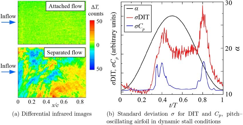
Meas. Sci. Technol. 31 (2020) 112002                                                                                         C Christian Wolf et al

Figure 1. Prediction of the transition location xtr on the upper (left) and lower (right) side of a trimmed rotor in forward flight, reproduced
from Heister [6].

project [8]. However, a conclusive validation of numerical                 temperature T∞ yields a convective heat flux q̇ depending on
tools would benefit from spatially well–resolved experimental              the local skin friction coefficient Cf ,
data including three–dimensional effects, which is apparent
                                                                                                     Cf   λ
from the predicted transition distributions shown in figure 1                                 q̇ =      U∞ (Tw − T∞ ) ,                        (1)
for a trimmed rotor at an advance ratio of 0.33.                                                     2    ν
   For turbomachinery aerodynamics, an unsteady inflow of                  with the external flow velocity U∞ , and the fluid’s thermal
the compressor or turbine blades in a rotor–stator layout is               conductivity λ and kinematic viscosity ν. The surface temper-
caused by the periodic wake of preceding stages, which also                ature Tw additionally depends on the conductive and radiative
results in moving BL transition [9, 10]. The transition not                terms, but a qualitative evaluation of the surface temperature
only affects the friction drag, but also the thermal loads of the          distribution Tw is usually sufficient to differentiate between the
blades. It is particularly difficult to access this type of flow           laminar and turbulent regions of the BL. This also means that
with sensors and measurement equipment, hence, many stud-                  a temperature calibration of the camera, depending the sur-
ies simplified the setup by investigating the influence of peri-           face emissivity and the heat flux sensor as described by Astar-
odic inflow perturbations on flat plates [11, 12], curved sur-             ita and Carlomagno [25], is not mandatory. The current work
faces [13], or stationary blade cascades [14]. In addition, early          will partly use the raw infrared signal in arbitrary camera units
fundamental research of moving BL transition on flat plates                (‘counts’) as synonym for the surface temperature. In recent
[15, 16] has currently been reviewed for fixed–wing aircraft               years IRT has become a standard tool for the detection of static
applications [17], assuming that low–frequency atmospheric                 transition positions. It was applied in wind tunnel testing of air-
turbulence may affect the performance of natural laminar–flow              foils [26, 27] or fixed–wing models [28], supersonic transition
airfoils.                                                                  measurements [29, 30], and in–flight measurements [31, 32].
   The blades of horizontal–axis wind turbines can easily be                   The current paper reviews recent developments of unsteady
subject to unsteady aerodynamics due to wind shear effects,                infrared thermography applied to moving boundary layer
yaw angles, interactions with the tower, or aeroelasticity                 transition measurements in unsteady inflow conditions. In
[18, 19]. It can be expected that these unsteady effects become            particular, the development of the differential infrared ther-
increasingly important in the future, given that the laminar               mography (DIT) at the German Aerospace Center (DLR) in
flow length is a crucial parameter of wind turbine airfoil design          Götingen is covered in chapter 4 and illustrated with examples
[20]. Another recent publication by Thiessen and Schülein                  and applications in the field of helicopter rotor aerodynamics.
[21] concentrated on moving transition positions due to the                The background to these activities is given by a summary of
effect of forward flight velocity on a fixed–pitch propeller for           other unsteady but non–infrared methods in chapter 2, and a
unmanned aerial vehicles.                                                  summary of steady infrared thermography in chapter 3 which
   Steady BL transition over a wetted surface can be measured              is the basis for unsteady measurements. Detailed considera-
by techniques which are well–known and understood. There                   tions of infrared radiation physics or camera technologies, see
are several experimental methods available, with infrared ther-            [25, 33], or infrared applications on other aerodynamic top-
mography (IRT) being one of the most convenient and most                   ics, such as heat flux measurements for super- and hypersonic
popular methods. IRT is non–intrusive and produces spatially               applications [34], are beyond the current scope.
resolved results in a two–dimensional measurement domain.
No instrumentation of the model is required, but in some cases,            2. Non–infrared methods for unsteady transition
an insulating surface coating must be applied depending on the             positions
base material. Pioneering work as described by Quast [22],
                                                                           2.1. Hot-film sensors
Carlomagno et al [23], or de Luca et al [24] developed the
underlying principle based on the Reynolds analogy. A small                The hot–film is a flush–mounted surface sensor that uses the
difference between the surface temperature Tw and the fluid                principle of constant temperature anemometry similar to the

                                                                       2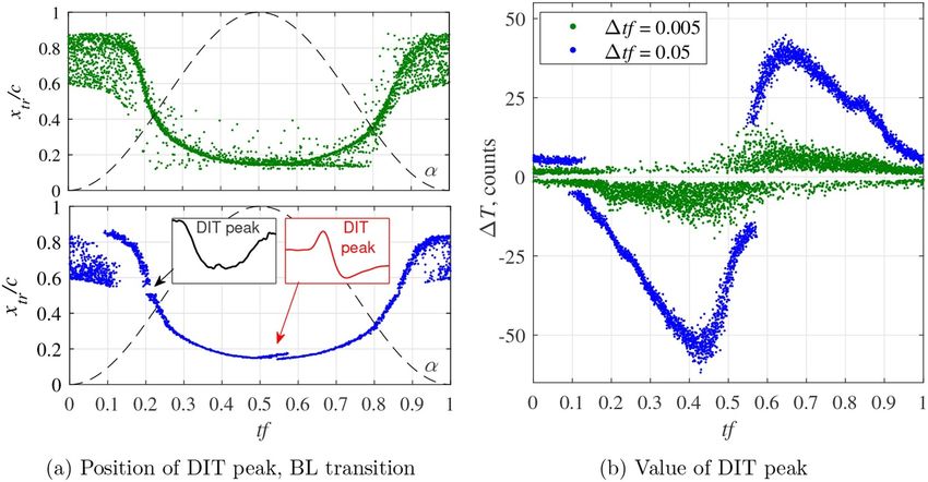
Meas. Sci. Technol. 31 (2020) 112002                                                                                       C Christian Wolf et al

well–known hot–wires. It is a standard method for measuring               cases, either due to the local surface heating, or the pressure
the wall shear stress over the Reynolds analogy for heat trans-           taps.
fer, also see equation (1), in a boundary layer [35, 36]. It can be           For impulsive, particularly hypersonic test facilities, the
used to detect dynamically moving boundary layer transition               hot–film gauges can be operated in an unheated mode, and are
[37], but can also distinguish between transition, stagnation             called thin–film gauges, see for example [54]. In this case the
point motion, flow separation, and shock formation [38]. The              ‘cold’ resistance of the sensor is related to the heat transfer
state of the literature for transition measurements on static air-        from the wall. The gauges have reaction times of the order of
foils with non-moving transition is particularly good, see for            microseconds, but to the authors’ knowledge were not yet used
example [39]. It should be noted that much of this literature             for dynamically moving boundary layer transition. An altern-
refers to the unsteady turbulent structures within the BL, see            ative to hot–films is to place hot–wires in the BL flow, and
for example [40], rather than a dynamically moving bound-                 indeed these offer advantages for some flow topologies, espe-
ary layer position as experienced by the pitching airfoil or the          cially for wake investigations [55] or for a rotating axisymmet-
helicopter rotor in forward flight.                                       ric cone [56].
    The pitching airfoil has been investigated for low–Mach
number airfoils [41–43] and for helicopter–relevant airfoils at
                                                                          2.2. Pressure sensors and microphones
Mach with compressible flow [38, 44, 45]. The investigations
of Richter et al involve 50 sensors on each airfoil, and are suit-        The σCP –method analyzes pressure signals from fast–
able for CFD calibration, see the comparisons in [46]. Hot–               response surface pressure transducers [57]. If the pressure
film sensors have also been extensively used for the investiga-           sensor signals are evaluated for an airfoil’s periodic pitch
tion of dynamically moving BL transition on laminar airfoils              motion, then the differences between different cycles will be
[47, 48], particularly in relation to aeroelastic flutter. Lorber         low in the laminar flow regions, medium in turbulent regions,
and Carta [49] did extensive investigations of the BL trans-              and a maximum near the transition position. This is because
ition and flow separation on a pitching airfoil, but the transition       slight differences in the wind tunnel operating conditions or
investigations involved only two sensors due to the low chord-            the pitch mechanism result in small cycle–to–cycle variations
wise resolution. For the rotating system, Sémézis [50] per-             of the moving transition position. Hence, in a certain phase
formed a hot–film investigation on the 7AD rotor and invest-              of the cycle, the transition position is in front of a given pres-
igations within the GOAHEAD project [8]. The data was also                sure sensor for some cycles but behind the sensor for the other
used for CFD validation [6]. A similar BL transition meas-                cycles. This increases the cycle–to–cycle standard deviation
urement using hot–films on an instrumented full–scale wind                of the pressure, σCp , since the transition affects the BL dis-
turbine blade was done by Schaffarczyk et al [51].                        placement thickness. A sample analysis of a pressure trans-
    The evaluation of hot–film data presents several difficulties,        ducer mounted to the suction surface of a rotor blade at 19%
which have increasingly been identified and at least partially            chord is shown in figure 3. Due to the chosen cyclic pitch amp-
solved in recent years. The first major problem is that for               litude, both the BL transition and the BL separation inducing
a dynamically moving BL transition, the transition intermit-              dynamic stall leave a footprint in the standard deviation of Cp .
tency is no longer seen as a transient stepping function. For a               The σCp –technique does not require a very high temporal
stationary BL transition region, a series of turbulent spots is           resolution of the pressure sensor as long as the overall aero-
generated and propagates past each sensor, and the fraction of            dynamics is properly captured. This is due to the fact that no
time in which the sensor is in the laminar or turbulent state             boundary layer modes are identified, but only the motion of the
is the experimentally defined intermittency. For the moving               transition position which is a broadband signal. The method
boundary layer, an increased RMS signal is present, but the               has been demonstrated for pitching airfoils at both high and
intermittency signal never appears, leaving the transition posi-          low inflow velocities [57, 59], and for pitching finite wings in
tion to be assessed through the soft step attained between lam-           both swept and unswept configurations [60, 61]. An applica-
inar and turbulent flow [52]. The step assessment also lends              tion to a rotor with cyclic pitch is also possible [62, 63] but the
itself to fully automated data processing (through data skew),            sensor integration requires additional effort, for example by
which solves the second problem of dealing with the large                 means of a telemetry system. Gao et al [64] and Wei et al [65]
amount of data required to include the sensor cut–off frequen-            proposed an approach which is similar to the σCp –idea but
cies of around 60 kHz [37, 52].                                           was developed independently. In their case, it was shown that
    An additional problem of hot–film sensors is that they                using a sliding window analysis rather than the cycle–to–cycle
involve an intrusion into the flow. Even if the sensor carrier            deviation yields transition results with a comparable quality.
foil is carefully kept to the same contour as the airfoil, the            Another evaluation strategy in literature is the M–TERA inter-
different surface roughness can result in a difference in the             mittency approach. It was originally formulated for velocity
transition position, see figure 2. For the same reason, the edges         fluctuations [66], but recently adapted to surface pressure fluc-
of the foil and the localized heating spots of the sensors may            tuations and transient inflow conditions [17]. The method must
cause disturbances. These influences can be reduced through               be seen as requiring additional validation.
good design and careful construction, but they can never be                   Microphones with a much broader frequency response than
completely avoided. Similarly, Mertens et al [53], noted that             the subsurface pressure sensors can also be used to detect
the regions of a pitching airfoil with pressure sensors had               BL transition, see [67, 68]. Microphones allow an analysis of
measurably different boundary layer transition for some test              boundary layer frequencies or modes of interest in addition to

                                                                      3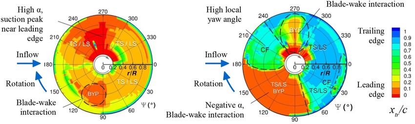
Meas. Sci. Technol. 31 (2020) 112002                                                                                       C Christian Wolf et al

Figure 2. Infrared images showing a difference of the transition position due to the presence of a hot–film foil, adapted from Richter et al
[46].

   Figure 3. σCp –analysis for a rotor blade with cyclic pitch input, f = 23.6 Hz, pitch amplitude Θ̂ = 6◦ , adapted from Schwermer [58].

the mere transition location, but with additional difficulties in         2.4. Direct skin friction measurements
analyzing the acoustics.
                                                                          Direct skin friction measurements provide the most desirable
                                                                          data for any boundary layer problem. A possible approach
2.3. Temperature–sensitive paint                                          is using sunk piezoelectric balances on which a small sur-
                                                                          face (‘movable wall element’) is mounted. The acquisition
Temperature–sensitive paint (TSP) is used in many of the same             of a moving boundary layer transition seems feasible, since
situations where infrared thermography can also be applied                small–floating mass, fast-response gauges are possible [76].
[69]. Under cryogenic conditions, TSP proved to be benefi-                However the practical difficulty of achieving the precise toler-
cial [70] in contrast to IRT due to the challenges of captur-             ances and low noise for this measurement mean that not much
ing the reduced radiated energy in the infrared spectrum [71].            data is available [77], and have not yet been used for moving
The surface preparation with the delicate paint layer requires            boundary layer transition. The sensors also have a temperat-
additional effort, and it offers the disadvantage that the sur-           ure and acceleration sensitivity which must be compensated.
face contour may be altered. The surface roughness of the                 Another method of skin friction measurement is given by
TSP can be very low if polished [72]. The data acquisition                shear–sensitive liquid crystals [78], but these have also not yet
using optical cameras allows a higher resolution compared to              been used for dynamically moving boundary layer transition.
infrared cameras, which enables a precise image dewarping
and a tracking of small-scale aerodynamic features. TSP can
                                                                          2.5. Comparison of different methods
be used for very short time exposures, see [73, 74]. The use
of difference–image techniques allows the use of TSP for the              Table 1 provides a short comparison of the most important
detection of dynamically moving BL transition, as applied on              measurement techniques for unsteady BL transition positions,
a slowly moving model during a pitch sweep test [75], but yet             listing their main advantages and disadvantages, and provid-
to be demonstrated on dynamically oscillating models.                     ing guidelines for the design of future experiments. Note that

                                                                      4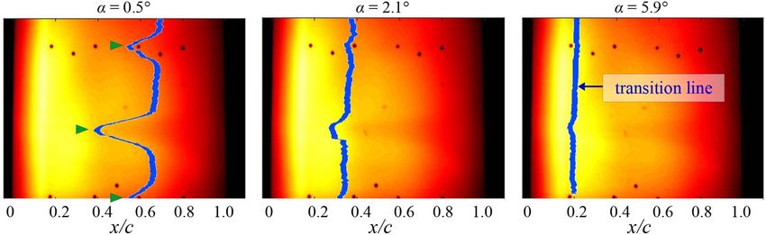
Meas. Sci. Technol. 31 (2020) 112002                                                                                      C Christian Wolf et al

                               Table 1. Main advantages and disadvantages of unsteady measurement techniques.

Method                                             Advantages                                     Disadvantages

Hot–film sensors                                  • Well–established and well–understood          • Extensive model preparation required,
                                                   measurement principle                           particularly for rotating surfaces (tele-
                                                  • Very high frequency range provides             metry or on–board systems)
                                                   deeper insight into the flow beyond            • Careful preparation of the experiment
                                                   transition position                             required (bridge balancing etc.)
                                                  • Suitable as reference for optical meas-       • Surface roughness and introduced heat
                                                   urement techniques                              probably affect flow
                                                  • Automated data analysis techniques            • Low spatial resolution
                                                   available, but different from steady–state
                                                   analysis

Pressure sensors                                  • Transition detection is a by–product of       • Extensive model preparation with care-
                                                   measuring pressure or lift distributions        ful sensor layout required, particularly
                                                  • Suitable as fast–response reference for        for rotating surfaces
                                                   optical measurement techniques                 • Subscale models require miniaturized
                                                  • Post–processing of acquired data is            sensors, often with limited or no possib-
                                                   simple and can be automated                     ilities for sensor repair
                                                  • Broadbanded response, robust to filter-       • Low spatial resolution
                                                   ing                                            • Pressure tap affects BL transition

Temperature sensitive paint                       • 2D measurement with very high resol-          • Surface coating on the order of 100 µm
                                                   ution possible                                  required
                                                  • Camera and optics equipment less              • Methods for unsteady measurements
                                                   costly than IR cameras                          under development, may require valida-
                                                  • Surface coating can be polished for            tion with reference technique
                                                   very low surface roughness

Unsteady infrared techniques                      • Comparably low effort for experi-             • Additional thermal measurement lag
                                                   mental setup and model preparation             • Requires temperature difference
                                                  • Particularly suitable for full–scale           between surface and flow, i.e. heating
                                                   applications                                   • Infrared spectrum is susceptible to
                                                  • Non–intrusive technique                        reflections from the measurement envir-
                                                  • 2D measurements with high resolution           onment
                                                   (but usually lower than TSP) possible          • Comparably new technique, may bene-
                                                                                                   fit from comparison to reference sensors

fast–response infrared techniques to be discussed in chapter 4            required by equation (1), and, if needed, a surface preparation.
are already included for the sake of completeness.                        The temperature difference can be achieved through:

                                                                          • Surface heating by external radiation flux sources: general
                                                                            purpose spotlights [63, 80], infrared emitter [81], infrared
3. Infrared thermography (IRT) for steady transition
                                                                            laser [21], or sunlight [68, 82].
positions
                                                                          • Surface heating by internal resistance heating: electrically
                                                                            conductive paint [83], carbon nano tube materials [84], heat
In comparison to other methods IRT enables convenient and                   foils [81], etc.
two–dimensional measurements of the BL transition location.               • Surface pre–heating [85, 86] or pre–cooling [82] for short–
Therefore, IRT is particularly suitable for full–scale in–flight            term tests.
measurements, as demonstrated by Horstmann et al [79] or                  • Inflow temperature: temperature–controlled laboratories or
Crawford et al [31, 32] on general aviation aircraft. With a                wind–tunnels, altitude changes during atmospheric flight
view to unsteady measurements in the following chapter, this                [32], etc.
section concentrates on applications with a stationary trans-
ition location due to steady inflow but fast–moving, particu-                The required temperature difference is often reported to
larly rotating surfaces.                                                  be on the order of several Kelvin but it depends on the setup
    The basic IRT setup consists of an infrared camera, a                 and the resulting signal–to–noise ratio, and no general recom-
strategy to achieve a fluid–surface temperature difference as             mendations can be made. The transition position itself may be

                                                                      5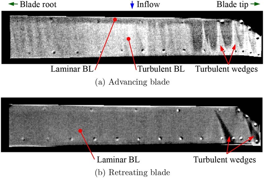
Meas. Sci. Technol. 31 (2020) 112002                                                                                          C Christian Wolf et al

affected if the heating is too strong, see Joseph et al [26] and
Costantini et al [87] for further recommendations.
    An insulating and dull coating can be applied to the surface
in order to reduce the thermal conductivity and to maximize
the infrared emissivity [25], which is mandatory for metallic
surfaces but optional for carbon fiber reinforced plastics. Fidu-
cial markers with differing radiation properties, for example
silver conductive paint, can be used to register and dewarp the
infrared images.
    The inherent motion blur in the infrared images must be
considered if a fixed ground–based camera is used to observe
fast–moving rotor blades. To the authors’ knowledge, no
infrared camera placement within the rotating frame has yet
been realized. Hub–mounted rotating cameras for the visible
light spectrum have been demonstrated [88, 89], requiring a
miniaturized camera size, a high tolerance towards centrifugal
forces, and a high resolution to perform image dewarp under
oblique viewing angles.
    Current infrared cameras are based on either thermal detect-
ors, which sense the incident energy flux, or quantum detect-
ors, which absorb incoming photons [25, 33]. The former
principle can, for example, be realized using mircobolo-
meter arrays, which is the cost–effective standard choice for
many cameras applied to steady–state BL measurements. The
required image exposure times are in the range of several mil-            Figure 4. Infrared image derotation in off–axis geometry [93].
liseconds [90] and, therefore, unsuitable to ‘freeze’ the motion
of rotor blades. Quantum detectors are used in high–speed
infrared cameras, featuring both a high repetition rate (f > 100        BL transition wedges due to leading edge erosion as a
Hz) and small image exposure times (∆t < 100µs). The sensor             by–product [92].
resolution is currently between about 0.2 Mpx and 0.5 Mpx,                  The rotational frequency of rotors or propellers for aircraft
which is at least one order of magnitude smaller than today’s           applications is large in comparison to wind turbines, particu-
visible–light cameras. The signal–to–noise ratio of the infrared        larly when investigating sub–scale models. The corresponding
images depends on the surface emissions, the camera exposure            motion blur can be reduced or avoided by optical blade track-
time, and its noise–equivalent temperature difference (NETD),           ing, as an additional measure complementing short–exposure
which is typically below 50 mK. The majority of the stud-               cameras. Rotating mirrors are suitable for this purpose if the
ies discussed in the following sections were conducted using            rotor hub position is stationary in a laboratory or wind–tunnel
either mercury cadmium telluride (MCT) or strained layer                environment. Several options for different mirror setups were
superlattice (SLS) sensors, both sensitive in the long–wave             discussed by Raffel and Heineck [93]. The easiest choice is to
infrared band (LWIR), or indium antimonide (InSb) sensors,              place the mirror axis collinear to the rotor axis, as applied by
sensitive in the mid-wave infrared band (MWIR). In practice             Overmeyer et al [94]. The image now follows the rotor blade
LWIR can be advantageous over MWIR since carbon fiber sur-              if the mirror frequency, fmirror , is half the rotor frequency, frotor .
faces are opaque in the long–wave regime and require no addi-           An off–axis configuration as shown in figure 4 can be useful
tional surface treatment.                                               when the mirror–camera–assembly may not obstruct the rotor
    Reichstein et al [68] successfully performed BL transition          shaft and the rotor inflow or outflow.
measurements on a 2 MW–wind turbine spinning at up to 9                     The infrared images are derotated over the entire blade span
rpm, combining ground–based infrared cameras of both MCT                if the mirror axis intersects the rotor axis at the hub including
and InSb types with blade–mounted microphones. The view-                an angle β, and the frequencies of mirror and rotor are related
ing distances of the cameras were 80 m and 140 m, with                  by:
image exposure times of about 100 µs. It is noted that many
large–scale measurements are limited by the scarce availab-                                                   1
                                                                                               fmirror =           frotor ,                     (2)
ility and high costs of telescopic lenses for infrared cameras.                                            2 cos β
Reichstein et al only observed small laminar flow lengths on
the blade’s suction side during nominal operation conditions            which is a generalization of the on–axis case (β = 0). The
of the wind turbine, but larger laminar lengths occurred dur-           chosen β should not be too large in order to minimize the
ing the transient spin–up of the rotor due to lower Reynolds            image distortion due to an oblique viewing angle. Addi-
numbers. A similar investigation was conducted by Dollinger             tionally, the periodicity between mirror     ( ) and rotor must be
et al [91]. Other wind turbine–related research focusing on             considered. For example, β = arccos 34 ≈ 41.4◦ results in
infrared on–site monitoring of structural blade defects found           frotor /fmirror = 32 . This means that repetitive images of the blade

                                                                    6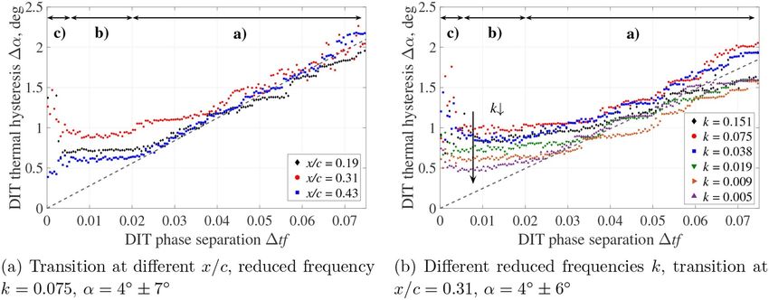
Meas. Sci. Technol. 31 (2020) 112002                                                                                    C Christian Wolf et al

                                                                       Figure 6. Infrared images of a ground–run test of an Airbus EC135
                                                                       rotor at 75% of the nominal rotor frequency, Richter and Schülein
                                                                       [82].

                                                                       signal–to–noise ratio to acquire the steady BL transition posi-
Figure 5. Mirror–derotated images of a rotor blade, adapted from
Heineck et al [95].                                                    tion. A large number of turbulent wedges is noted due to con-
                                                                       tamination or surface defects at the leading edge.

at the same azimuth angle and with the same viewing geometry 4. Unsteady measurements and differential infrared
can be taken every third revolution of the rotor corresponding thermography (DIT)
to every second revolution of the mirror. This choice is a good
compromise between the different requirements, and was for 4.1. Principle, pitching airfoil measurements, and
                                                                   optimization
example chosen by Weiss et al [63].
    Heineck et al [95] applied IRT and mirror–based derotation The effects of unsteady inflow conditions on infrared BL trans-
to the lower side of a two–bladed rotor with a radius of R = 0.9 ition measurements of a wetted surface can be divided into
m, spinning at f = 15 Hz in the hover chamber at NASA Ames. three categories:
The large duration of image exposure, 4.5 ms, covered an azi-
                                        ◦
muthal blade motion of ∆Ψ = 24 , but the rotating mirror            (i) Inviscid aerodynamics govern the time–dependency
facilitated sharp infrared images, see figure 5. The blade was          between the inflow conditions and the surface pressure
radiation–heated by a 1 kW–lamp in the lower image. Hence,              distribution. For example considering pitch–oscillating
the turbulent BL in the rear section of the blade is colder             airfoils, Theodorsen’s theory [96] predicts a hysteresis
due to the stronger heat convection, and it appears in darker           between the pitch angle and the lift force due to differen-
coloring. Fiducial markers used for image registration were             tial velocities induced by shed vorticity in the wake.
placed in regular intervals near the leading edge, resulting in (ii) Viscous effects may introduce an additional hysteresis
turbulent wedges. The interpretation of the infrared images is          between an airfoil’s pressure distribution and the bound-
identical to static airfoil tests since the aerodynamics is steady      ary layer’s transition position. This effect was shown by
in the rotating frame. The upper image is without heating.              Richter et al [45] for a pitching airfoil, and confirmed by
The transition–related coloring is inverted in comparison to            Gardner et al [61].
the lower image, since the blade was slightly colder than the (iii) The thermal responsiveness, comprising the thermal dif-
heating–up environment, but the pattern has a much lower con-           fusivity and the specific heat, connects the boundary
trast.                                                                  layer’s instantaneous convective heat transfer with the
    This basic setup was further improved in subsequent meas-           surface temperature as acquired by an infrared camera.
urement campaigns, but rotating mirrors were partly omitted,
since newer camera generations offered an improved signal–             The ‘true’ aerodynamic transition position only includes
to–noise ratio at small exposure times. It is noted that meas- effects (i) and (ii), whereas effect (iii) is an error which must be
urements of unsteady aerodynamics still benefit from mirror eliminated or reduced by the infrared measurement technique.
derotation, as shown in the next chapter. Setups with two IR           When the aerodynamic unsteadiness is sufficiently slower
cameras examining both upper and lower blade surfaces were than the thermal responsiveness, steady–state evaluation meth-
applied by Richter et al [85] during ground tests of a prototype ods can still be applied. This was shown by Szewczyk et al
full–scale helicopter rotor, and Overmeyer and Martin [83] on [97], observing the BL transition on a glider wing during
a Mach–scaled model helicopter rotor.                              a stall–and–recovery maneuver lasting about eight seconds.
    Richter and Schülein [82] measured the BL transition on Simon et al [81] discuss the frequency response of infrared
both large–scale model rotors operated on whirl towers, and transition measurements for several surface materials and heat
full–scale helicopter rotors during ground–run and hover- sources, with response times in the range of several seconds to
ing test cases. The infrared camera was mounted obliquely minutes.
above the rotor plane viewing the blade’s upper surface, see           A possible evaluation strategy to overcome thermal hyster-
figure 6. The image exposure time of down to 20 µs was esis effects (iii) is differential infrared thermography (DIT),
small enough to avoid motion blur while ensuring a sufficient which was proposed by Raffel and Merz [98] and Raffel

                                                                   7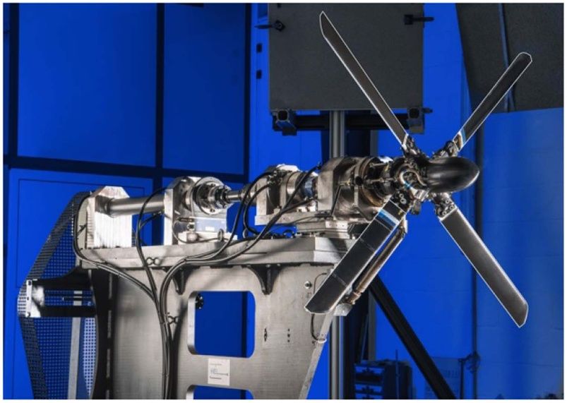
Meas. Sci. Technol. 31 (2020) 112002 C Christian Wolf et al
et al [99]. The DIT principle is introduced in figure 7, with Hoesslin et al [102] proposed a concept similar to DIT
a more detailed description following in the next sections. The with a view to turbomachinery applications. In their case, the
infrared images, left and center, were taken successively dur- surface temperature’s decline rate after an impulsive flash is
ing the pitch up–motion of a rotor blade. The aerodynamic– measured using high–repetition rate infrared images, which
related features are gradual variations of the infrared intens- also visualizes the differing heat convection before and after
ity in chordwise direction, and a prominent turbulent wedge BL transition. The concept should also enable short–term
caused by a transition dot. The differential image in figure 7, measurements, but so far, only steady airfoil results were pub-
right, clearly reveals the transition moving forward between lished.
both time instants, as seen by a dark band representing decreas- The basic principle of DIT was validated and refined in
ing temperatures due to increased cooling. The spanwise vari- several measurement campaigns for quasi two–dimensional
ation of the transition is due to three–dimensional effects close and pitching airfoils. Richter et al [46] compared DIT to hot–
to the blade tip. film data and to the σCp –method [103] based on fast–response
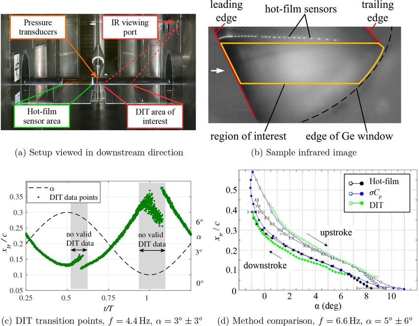
The difference between steady and unsteady infrared meas- surface pressure transducers. The results cover the DSA-9A
urements can be seen in figure 8. Figure 8(a), top, shows helicopter airfoil tested in the Transonic Wind Tunnel Göt-
the chordwise infrared signal of an airfoil’s quasi two– tingen, see figure 9(a), at M = 0.3, Re = 1.8 · 106 and differ-
◦
dimensional upper surface at static pitch angles, α, of 4.0 ent pitch frequencies up to 8.8 Hz. The infrared camera was a
◦
and 4.5 . The airfoil was radiation–heated so that the surface FLIR SC 7750-L LWIR MCT, sensitive in the spectral range
temperature, Tw , was slightly above flow temperature. The of 8.0 − 9.4 µm, and combined with a 50 mm focal length–
transition region is located at about 0.25 < x/c < 0.35, where lens. The native sensor size was cropped to 640 × 310 px,
the surface temperature strongly decreases due to an increas- enabling an acquisition frequency of 190 Hz at an integration
ing convective heat transfer. The steepest gradient dT/dx rep- time of 100 µs. Images of the model’s untreated CFRP sur-
resents 50% intermittence [80]. face were taken through a germanium window in the tunnel’s
Subtracting both static temperature distributions results in side wall, see figure 9(b). The hot–film sensors are visible as
the differential signal ∆T shown in figure 8(a), bottom. The bright spots and can be used for image registration, hence, no
transition moves forward with increasing α, creating a negat- fiducial markers were needed. The model was heated with a
ive peak at xtr ≈ 0.28 which can be attributed to 50% inter- 2 kW–spotlight mounted outside of the opposite side wall, and
mittence at the mean pitch of (4.0◦ + 4.5◦ )/2 = 4.25◦ . Inter- differential images of subsequent time steps were calculated.
preting ∆T is unambiguous, since secondary effects related to The DIT signal was averaged in spanwise direction, and the
uneven heating, to the external flow, or to inhomogeneities in peaks were detected similar to figure 8(b).
the airfoil’s material composition are canceled out. However, Figure 9(c) shows the DIT transition data (green dots) as a
it was observed that reflections from the environment of the function of the phase t/T for a sinusoidal pitch motion (dashed
model must be carefully avoided, since the reflection’s posi- black line) taken during multiple pitch cycles. Each data point
tion on the model surface may shift during pitch angle vari- represents the location xtr of a differential peak, with the
ations, creating apparent and erroneous differential signals. peak being either positive or negative depending on whether
Reflections can be prevented by a careful selection of the cam- the transition moves forward or backward. During motion
era position and by using anti–reflective background material reversal, see the gray areas in figure 9(c), the DIT results are
such as cloth curtains. unreliable due to a diminishing signal strength. This problem
Infrared measurements at the same pitch angles but taken will treated in the next sections in more detail. Post–processing
during a sinusoidal pitch motion are shown in figure 8(b). The can be applied to remove outlier and to calculate the phase–
thermal inertia of the model’s CFRP surface is not negligible averaged transition location. The three experimental methods
compared to the pitch frequency of 2 Hz. Hence, the distribu- yield similar results, see figure 9(d), with deviations below
◦ ◦
tions at α = 4.0 and α = 4.5 are very similar, and the steepest 10% of the chord length for this setup. The split between up-
temperature gradient does no longer coincide with the instant- and downstroke due to hysteresis effects is largest for DIT,
aneous transition position. A similar observation is reported by which is a result of the additional measurement lag (iii) due to
Ikami et al [100] using temperature sensitive paint on a pitch- the surface’s thermal responsiveness. The other methods are
ing airfoil. However, the peak of the differential signal ∆T supposed to cover only the ‘true’ aerodynamics (i) and (ii).
is still a valid indicator for xtr , even though the peak level is Wolf et al [80] revisited the sinusoidally pitching air-
about five times smaller compared to the static measurement. foil model of Richter et al [46] in the low–speed ‘1-meter’
Since the unsteady measurements were taken during the pitch wind tunnel at DLR Göttingen, using the same MCT infrared
upstroke, the transition position of xtr ≈ 0.295 is delayed in camera and a similar radiation heating with a flux rate in
downstream direction due to hysteresis in comparison to the the range of 500 − 1500 W/m2 over the suction surface.
static value of xtr ≈ 0.28. It is noted that early DIT publications The inflow Mach and Reynolds numbers were lowered to
[99] proposed to not only interpret the DIT peak position but M = 0.14 and Re = 1 · 106 , increasing the BL’s laminar length
also the width of the peak, connecting the peak’s base points at a given lift coefficient. The low–speed tunnel enabled
to the start and end of the intermittency region. However, it is cost–effective parameter studies and optimizations of the
difficult to identify the base points in the presence of random DIT method. A sketch the setup is in figure 10, which can
measurement noise, and aerothermal simulations of pitching be taken as a blueprint for similar pitching–airfoil studies
airfoils [101] later disproved the concept. [59, 98, 99].
8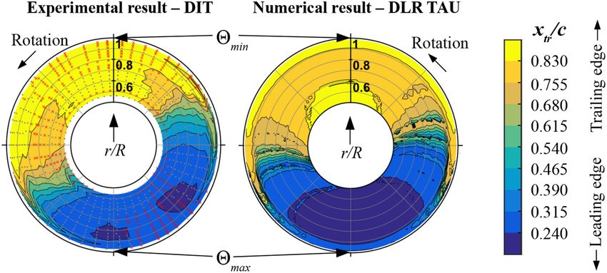
Meas. Sci. Technol. 31 (2020) 112002                                                                                    C Christian Wolf et al

                                         Figure 7. DIT principle, adapted from Raffel et al [99].

               Figure 8. Infrared measurements on the DSA-9A helicopter airfoil, U∞ = 50 ms−1 , data from Wolf et al [80].

   The main focus of Wolf et al’s investigation was set on              is corrupted and slightly biased by temperature drift in case
the influence of the separation distance between two infrared           of the unfiltered signal. In contrast, the filtered signal shows a
images to be subtracted, which can be expressed as a time dif-          clear peak in the transition region and is nearly zero elsewhere.
ference ∆t, or, assuming a periodic pitching motion with fre-              The airfoil’s DIT transition analysis for sinusoidal pitch
                                                                                                               ◦
quency f, as a phase difference ∆tf. It was shown that it is            oscillations with an amplitude of 7 and a reduced frequency
favorable to detune the acquisition frequency of the infrared           of k = πfc/U∞ = 0.075 (f = 4 Hz) is shown in figure 12. The
camera from the aerodynamic periodicity f with its multiples.           green and blue dots correspond to separations of ∆tf = 0.005
Now combining the infrared images of a large number of                  and ∆tf = 0.05, respectively. The smaller separation captures
acquired pitch cycles provides a high resolution of the phase           the general motion of the transition well, as seen in figure 12(a)
angle, and allows to optimize the phase difference ∆tf. In this         (top). The transition position on the upper surface is close
example, a camera frequency of 99.98 Hz yields a phase resol-           to the leading edge at high pitch angles around tf = 0.5 but
ution of ∆tf = 2 · 10−4 . Since the transition–related peaks of         close to the trailing edge at low pitch angles around tf = 0 and
∆T are usually well below 1 K, this approach requires remov-            tf = 1. It is noted that the shape of the transition motion is not
ing the long–term temperature drift, which even in a laborat-           sinusoidal, since the relation between α and xtr is not linear
ory environment cannot be avoided, and which may vary with              and depends on the airfoil shape. However, the random scat-
the spatial coordinates due to the model’s internal structure or        ter of the small separation ∆tf is large since the subtracted
inhomogeneous heating. This is shown in figure 11, in which             infrared images are very close, and the resulting DIT peak val-
the black line is a sample unfiltered DIT signal as a func-             ues shown in figure 12(b) are barely above the camera’s noise
tion of the chordwise coordinate. The underlying phase dif-             level. The ratio between peak values and underlying measure-
ference is small, ∆tf = 0.05 corresponding to 5% of the pitch           ment noise is crucial for the achievable spatial and temporal
period, but both images were taken from different pitch cycles          resolution of the DIT analysis. The random scatter is reduced
with a wall–clock difference of about 40 s. The red line is the         for large DIT image separation, see figure 12(a) (bottom). This
high–pass filtered DIT signal, using a cut–off time twice the           corresponds to an increased peak signal strength as in figure
length of the pitching period. The transition–related peak at           12(b), with the negative or positive sign of the peak depending
x/c ≈ 0.15 (green arrow) is visible in both distributions, but it       on whether the motion is towards the leading or trailing edge.

                                                                    9
Meas. Sci. Technol. 31 (2020) 112002 C Christian Wolf et al
Figure 9. Transition measurements on a pitching airfoil using three experimental methods, see Richter et al [46].
Figure 10. Sketch of a DIT wind–tunnel setup [80].
Figure 11. DIT temperature drift correction using a high–pass filter
[80].
Despite the large separation, the differential signal dimin-
ishes towards the frontmost and backmost positions where the
movement of the transition is slower. Particularly at tf = 0.5, positive and negative peaks. Assuming that the peak search
the same bifurcation as in figure 9(c) is observed. This bifurc- algorithm detects the maximum peak value regardless of its
ation can be attributed to a DIT double–peak structure, see the sign, the results will randomly switch between both states, cre-
red detail in figure 12(a) (bottom), with a coexistence of both ating the bifurcation. A detailed analysis in the next section
10Meas. Sci. Technol. 31 (2020) 112002 C Christian Wolf et al
Figure 12. DIT analysis of a pitching airfoil, suction surface, k = 0.075, α = 4◦ ± 7◦ , DIT separation ∆tf = 0.005 (green dots) and
∆tf = 0.05 (blue dots), see [80].
will show that the true transition position is in between. At the unsteady heat transfer in the airfoil’s wall–normal direc-
tf = 0.2, the large separation of ∆tf = 0.05 produces another tion, allowing the evaluation of synthetic temperature distribu-
gap in the transition data. This can be attributed to a broad tions and derived DIT results. The study generally confirmed
negative–negative DIT double–peak structure, see the black the validity of the DIT method, but also provided new insight
detail in figure 12(a) (bottom). At this chordwise position the into problems connected to the thermal responsiveness. Fig-
transition motion is fast and the intermittency regions in both ure 14 shows the predicted chordwise differential temperat-
infrared images no longer overlap, hence, the single DIT peak ure distributions, ∆T, before and after the reversal of the pitch
starts to split up into two separate peaks. motion at the minimum pitch angle, corresponding to a phase
This raises the question of the optimal infrared image sep- of ft = 0.
aration ∆tf, with figure 13 showing the influence of ∆tf on The sign of the peak expectedly changes from positive to
the parasitic measurement hysteresis (iii). This hysteresis is negative. When the motion of the transition stops in its most
defined as the pitch difference, ∆α, between the up- and rearward position at about x/c = 0.55, the ∆T–signal should
downstroke for a given transition position. The true aerody- be zero for a surface material with infinite responsiveness and
namic hysteresis as seen by the σCp –method was subtracted, no thermal lag. When introducing a finite thermal responsive-
so ∆α = 0 means an error–free DIT measurement. The hys- ness, both positive and negative peaks are coexistent, which
teresis depends on multiple factors such as the pitch motion, is particularly visible for the dark blue line at ft = 0.021. This
the airfoil’s geometry and surface material, the infrared cam- simulation result has a strong qualitative resemblance to the
era’s signal–to-noise ratio, etc. For a variation of the transition experimental differential signal shown in the red detail in fig-
position, figure 13(a), and a variation of the reduced pitch fre- ure 12(a) (bottom). The ‘double–peak’–structure yields sys-
quency k, figure 13(b), three universal effects can be identi- tematic errors, which explain the bifurcation of the DIT data
fied: In region a) the measurement hysteresis decreases with points observed in the gray areas of figures 9(c) and 12(a) (bot-
decreasing phase separation, since the subtracted infrared sig- tom). The true aerodynamic transition positions marked by
nals successively converge on the instantaneous state of the dots in figure 14 are between the positive and negative peaks,
flow. The minimum measurement hysteresis, limited by the and they do not coincide with the detected ‘phantom’ peaks
thermal responsiveness of the airfoil’s surface, is reached in marked by the dashed black locus curve.
region b). A further reduction of the separation in region c) Gardner et al [101] further investigated the effects of dif-
yields an increasing scatter and measurement uncertainty since ferent surface materials, assuming that the DIT measurements
the diminishing temperature difference between to images benefit from both a low thermal diffusivity and a low spe-
approach the camera’s noise limit. cific heat. The results shown in figure 15 are referenced
Gardner et al [101] conducted a 2D URANS simulation of to the epoxy matrix material used for the CFRP model in
Richter et al’s [46] and Wolf et al’s [80] experiment, including Richter et al [46]. Even the best insulators, expanded poly-
aerodynamic hysteresis effects. The predicted instantaneous styrene and cork, offer only moderate reductions in terms of
skin friction coefficient Cf was coupled to a 1D simulation of DIT thermal delay representing the hysteresis (top graph).
11Meas. Sci. Technol. 31 (2020) 112002 C Christian Wolf et al
Figure 13. Thermal hysteresis ∆α as a function of the DIT image separation ∆tf, see [80].
Figure 14. Synthetic DIT results at the reversal of the pitch motion,
f = 6.6 Hz, α = 5◦ ± 6◦ , see [101]. Figure 15. Comparison of surface materials, relative DIT thermal
delay (top) and signal strength (bottom), adapted from Gardner et al
[101].
On the other hand, the peak strength of ∆T can be signific-
antly increased by a factor of 10 and more (bottom graph).
This result motivates the application of surface coatings, as to the thermal responsiveness. A high phase resolution of
it was also shown that the unsteady temperature variations the infrared images allows the analysis of the temperature T
are restricted to a very thin surface layer with a thickness at a given position x/c over the entire pitch cycle. This is
below 0.5 mm. On the other hand, the coating’s application, shown in figure 16, left, in which the temperature signal at
its mechanical strength, and its surface roughness have to be x/c = 0.31 was low–pass filtered with sliding average window
considered. sized ∆tf = 0.02 (2% of the pitch cycle) to reduce noise. The
Based on these observations and using the same experi- convective cooling effect of the turbulent BL is clearly seen
mental setup [80] Mertens et al [53, 104] proposed that the by means of a decreasing temperature between about tf = 0.24
image separation should be optimized with respect to a qual- and tf = 0.78. The transition passes slightly after the temper-
ity indicator which accounts for data scattering. This approach ature peaks, see the square symbols in figure 16 (left), but
is particularly suitable for sinusoidal pitch motions, in which before the peaks of the numerically derived temperature gradi-
the speed of the transition motion and the corresponding dif- ent dT/d(ft), see the circular symbols in figure 16 (right). It is
ferential infrared signal strongly varies over the pitch cycle. noted that analyzing this local temperature gradient is equi-
Mertens et al [53] also proposed local infrared thermo- valent to the DIT approach with a very small image separation
graphy (LIT) as a variant of DIT which adds further insight ∆tf. LIT reduces the data scatter noted in the DIT results of
12Meas. Sci. Technol. 31 (2020) 112002 C Christian Wolf et al
Figure 16. LIT, local temperature (left) and local temperature gradient (right) at x/c = 0.31 for k = 0.075 and α = 4◦ ± 6◦ [53].
figure 13 for ∆tf → 0 by applying the aforementioned sliding The first successful application of DIT to a subscale
window filter. rotor was demonstrated at the rotor test stand Göttin-
Using optimized evaluation procedures and infrared data gen (RTG) by Raffel et al [99], providing data on mov-
with a good signal–to–noise ratio, it is possible to extend the ing BL transition for unsteady conditions complementing
differential analysis to produce two–dimensional results down earlier steady–state test cases [74, 105]. The RTG, see fig-
to the resolution of a single pixel [53, 104]. This particularly ure 18, enables an azimuth–varying blade pitch through
avoids taking the spanwise average of airfoils as in [46, 80]. a swashplate similar to helicopters, but it has a hori-
Figure 17 shows the two–dimensional LIT analysis during the zontal axis and does not simulate edge–wise inflow as
upstroke of a sinusoidal pitch motion, considering the airfoil’s in helicopter forward flight. The RTG is optimized for
suction side with the flow from left to right. The detected trans- the synchronized application of blade–mounted sensors,
ition area is marked in blue color and superimposed onto the such as pressure transducers, and external optical camera
original infrared image data. For an increasing pitch angle, left systems.
to right, the transition moves towards the leading edge. The A similar test with an improved setup and rotor frequen-
smallest pitch angle, figure 17 (left), shows three–dimensional cies up to 23.6 Hz was conducted by Weiss et al [63]. The
effects by means of a slightly tilted BL transition line interrup- application of a high–speed infrared camera and a rotating mir-
ted by three transition wedges marked by green triangles. The ror allowed the acquisition of both DIT measurement images
top and bottom wedges result from an increased surface rough- to be subtracted during a single rotor revolution with a con-
◦
ness due to the painted fiducial markers appearing as black stant azimuthal separation of ∆Ψ = 18 , corresponding to
dots in the images. The central wedge is caused by surface a phase separation of ∆tf = 0.05 and an image frequency
pressure taps which are not seen by the infrared camera. In of 472 Hz. The camera was a FLIR X8500sc SLS LWIR,
this chordwise area small perturbations have a strong influence which is sensitive in the spectral range of 7.5 − 12 µm. The
on the transition position due to the flat pressure distribution. image integration time was set to 57 µs, which is lower
Towards the leading edge, the transition is mainly caused by in comparison to the MCT camera used in [80, 99] due to
the strong pressure gradient dp/dx downstream of the suction a superior signal–to–noise ratio (NETD: 20 mK versus 35
peak. Hence, the influence of surface defects is smaller, and mK). The spatial resolution was 2 mm/px using a 50 mm
the transition line becomes more two–dimensional as in figure focal length–lens. The radiative heat flux provided by halogen
17 (right). lamps was about 400 − 500 W/m2 , which is on a similar level
as in [80].
DIT transition results for the suction side of the rotor blade
and at a radial station of r/R = 0.8 are shown as black dots in
4.2. Rotor measurements
figure 19. The unsteady inflow conditions were produced by a
◦
Measurements of unsteady BL transition locations on rotat- cyclic swashplate setting with a pitch amplitude of about 6 ,
ing or fast–moving aerodynamic surfaces is one of the most and the data is similar to pitching–airfoil data shown in the pre-
challenging tasks for infrared thermography, since most of the ceding section. A comparison to steady–state IRT results at the
difficulties described in the earlier sections add up. corresponding constant pitch angles, marked by blue squares
13Meas. Sci. Technol. 31 (2020) 112002 C Christian Wolf et al
Figure 17. LIT transition measurement in a 2D–domain, pitching airfoil (upstroke), suction surface, k = 0.075, α = 4◦ ± 6◦ [53].
The combined results at the radial stations between
r/R = 0.4 and 1.0 can be visualized in a polar coordinates,
forming the transition map shown in figure 20 (left). The
experimental data is compared to a numerical DLR TAU simu-
lation of the experiment in figure 20, right. The simulation was
set up based on the best practices described by Kaufmann et al
[106], and the overall agreement of the BL transition position
xtr is very good. The minimum and maximum pitch angles are
at the top and bottom of the rotor plane maps, respectively.
Note that the transition pattern, with light colors indicating xtr
close to the trailing edge and dark colors indicating xtr close
to the leading edge, is roughly symmetric but slightly rotated
in counterclockwise direction representing aerodynamic hys-
teresis effects.
The model–scale measurements provide a rough estimate
for the operating range of DIT using current infrared camera
Figure 18. Rotor test stand at DLR Göttingen (RTG). technology. Figure 21 shows the DIT thermal hysteresis (iii)
as an excess pitch ∆Θ over the true aerodynamic hysteresis,
corresponding to the definition used in figure 13. The data of
references [46, 63, 80] is plotted as a function of the airfoil’s
or blade’s pitch rate. For decreasing pitch rates below about
◦
15 /s, see the detail in the right figure, the thermal hysteresis
monotonically decreases towards zero, representing an error–
free transition measurement for static conditions. For larger
and technically relevant pitch rates the thermal hysteresis is
◦ ◦ ◦
bounded by about 1 to 1.5 , neglecting a single outlier at 2.3
[63]. Nevertheless, the DIT principle was demonstrated even
◦
for very high pitch rates up to almost 900 /s. It is noted that the
stated thermal pitch hysteresis ∆Θ cannot be generally con-
verted into a bias of the detected transition position, since the
corresponding transition motion highly depends on the airfoil
shape.
Overmeyer et al [94] conducted the first BL transition
measurement of a trimmed rotor in forward flight conditions,
applying DIT to the lower side of the three–bladed NASA PSP
Figure 19. RTG transition position at r/R = 0.8, IRT results for
model rotor with a radius of 1.7 m. The rotor was operated
static pitch angles, DIT results for cyclic pitch input, f = 23.6 Hz,
in the Langley 14 × 22–Foot Subsonic Tunnel at f = 18.2 Hz
pitch amplitude Θ̂ = 6◦ [63].
and advance ratios up to µ = 0.38. DIT images were calcu-
lated by subtracting dewarped infrared images with an azi-
◦
in figure 19, reveals the aerodynamic hysteresis by means of a muthal spacing of about 23 . The interpretation of the res-
shift towards larger phases tf, that is, towards the right side. ults is different compared to the preceding sections due to the
14You can also read