Measuring the labor market at the onset of the COVID-19 crisis - Brookings ...
←
→
Page content transcription
If your browser does not render page correctly, please read the page content below
BPEA Conference Drafts, June 25, 2020

Measuring the labor market at the onset of the
COVID-19 crisis

Alexander W. Bartik, University of Illinois at Urbana-Champaign
Marianne Bertrand, University of Chicago
Feng Lin, University of Chicago
Jesse Rothstein, University of California, Berkeley
Matthew Unrath, University of California, Berkeley
Conflict of Interest Disclosure: The authors did not receive financial support from any firm or person for this
paper or from any firm or person with a financial or political interest in this paper. The authors utilized data
provided by Homebase, which was made available to a large number of academics and has not been restricted
in its use in any way. They are currently not officers, directors, or board members of any organization with
an interest in this paper. No outside party had the right to review this paper before circulation. The views
expressed in this paper are those of the authors, and do not necessarily reflect those of the University of
California, Berkeley, the University of Chicago, or the University of Illinois, Urbana-Champaign.

Measuring the labor market at the onset of the COVID-19 crisis*

                  Alexander W. Bartik, University of Illinois at Urbana-Champaign
                             Marianne Bertrand, University of Chicago
                                 Feng Lin, University of Chicago
                        Jesse Rothstein, University of California, Berkeley†
                        Matthew Unrath, University of California, Berkeley

                                                  June 2020

Abstract
We use traditional and non-traditional data sources to measure the collapse and subsequent partial
recovery of the U.S. labor market in Spring 2020. Using daily data on hourly workers in small
businesses, we show that the collapse was extremely sudden -- nearly all of the decline in hours of
work occurred between March 14 and March 28. Both traditional and non-traditional data show
that, in contrast to past recessions, this recession was driven by low-wage services, particularly the
retail and leisure and hospitality sectors. A large share of the job loss in small businesses reflected
firms that closed entirely. Nevertheless, the vast majority of laid off workers expected, at least
early in the crisis, to be recalled, and indeed many of the businesses have reopened and rehired
their former employees. There was a reallocation component to the firm closures, with elevated
risk of closure at firms that were already unhealthy, and more reopening of the healthier firms. At
the worker-level, more disadvantaged workers (less educated, non-white) were more likely to be
laid off and less likely to be rehired. Worker expectations were strongly predictive of rehiring
probabilities. Turning to policies, shelter-in-place orders drove some job losses but only a small
share: many of the losses had already occurred when the orders went into effect. Last, we find that
states that received more small business loans from the Paycheck Protection Program and states
with more generous unemployment insurance benefits had milder declines and faster recoveries.
We find no evidence so far in support of the view that high UI replacement rates drove job losses
or slowed rehiring substantially.

*
  Prepared for the Brookings Papers on Economic Activity conference on June 25, 2020. We thank Justin Germain,
Nicolas Ghio, Maggie Li, Salma Nassar, Greg Saldutte and Manal Saleh for excellent research assistance. We are
grateful to Homebase (joinHomebase.com), and particularly Ray Sandza and Andrew Vogeley, for generously
providing data.
†
  Corresponding author. rothstein@berkeley.edu.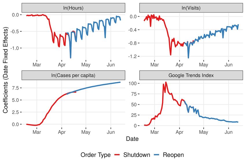
I.   Introduction

The COVID pandemic hit the U.S. labor market with astonishing speed. The week ending March
14, 2020, there were 250,000 initial unemployment insurance claims -- about 20% more than the
prior week, but still below January levels. Two weeks later, there were over 6 million claims. This
shattered the pre-2020 record of 1.07 million, set in January 1982. At this writing, claims have
been above one million for thirteen consecutive weeks, with a cumulative total of over 40 million.
The unemployment rate shot up from 3.5 percent in February to 14.7 percent in April, and the
number of people at work fell by 25 million.

The United States labor market information systems are not set up to track changes this rapid.1
Our primary official indicators about the state of the labor market come from two monthly surveys,
the Current Population Survey (CPS) of households and the Current Employment Statistics (CES)
survey of employers. Each collects data about the second week of the month, and is released early
the following month. In 2020, an enormous amount changed between the second week of March
and the second week of April.

In this paper, we attempt to describe the labor market in what may turn out to be the early part of
the COVID-19 recession. We combine data from the traditional government surveys listed above
with non-traditional data sources, particularly daily work records compiled by Homebase, a private
sector firm that provides time clocks and scheduling software to mostly small businesses. We link
the Homebase work records to a survey answered by a subsample of Homebase employees. We
use the Homebase data to measure the high-frequency timing of the March-April contraction and
the gradual April-May recovery. We use CPS and Homebase data to characterize the workers and
businesses most affected by the crisis. And we use Homebase data as well as data from other
sources (e.g., on physical mobility) to measure the effects of state shelter-in-place orders and other
policies (in particular, the Paycheck Protection Program and unemployment insurance generosity)
on employment patterns from March to early June.

1
  In response to the limitations of traditional data sources, the Census Bureau started Household Pulse and Business
Pulse surveys to provide higher frequency data on changes in the labor market and for small businesses. These
surveys provide very useful information going forward, but only started on April 23rd and 27th respectively, and so
are limited in their ability to understand the start of the COVID-19 economic disruptions.
                                                                                                                   2
We are not the only ones studying the labor market at this time. Cajner et al. (2020; in this volume),
Allcott et al. (2020), Chetty et al. (2020), Cortes and Forsythe (2020), Dey et al. (2020); Gupta et
al. (2020), Khan et al. (2020), Kurmann et al. (2020), Mongey et al. (2020) and Lin and Meissner
(2020) conduct exercises that are closely related to ours. There are surely many others that we do
not cite here. Our goal is neither to be definitive nor unique, but merely to establish basic stylized
facts that can inform future research on the crisis.

The paper proceeds as follows. Section II describes the data sources. Section III provides an
overview of the labor market collapse and subsequent partial recovery. In Section IV, we explore
who was affected by the collapse, investigating characteristics of workers that predict being laid
off in March and April, then being reemployed thereafter. Section V uses event study models to
examine the effects of non-pharmaceutical interventions (i.e., shelter-in-place and stay-at-home
orders) on hours worked in the Homebase data. To contextualize these effects, we also show
impacts on Google search behavior, on visits to commercial establishments, and on COVID-19
case diagnoses. Section VI examines the impacts of the roll-out of unemployment insurance
expansions at the state level and of the Paycheck Protection Program on Homebase hours. We
conclude in Section VII.

 II.   Data

We rely on two primary sources to measure the evolution of the labor market during the first half
of 2020, supplementing with a few labor and non-labor-market measures that provide useful
context.

First, we use the Current Population Survey (CPS), the source of the official unemployment rate.
This is a monthly survey of about 60,000 households conducted by the Census Bureau in
collaboration with the Bureau of Labor Statistics. Respondents are surveyed during the week
containing the 19th of the month, and asked about their activities during the prior week (the week
containing the 12th). The most recent available data are from the May survey. The CPS sample
has a panel structure, with the same households interviewed for several consecutive months. This

                                                                                                    3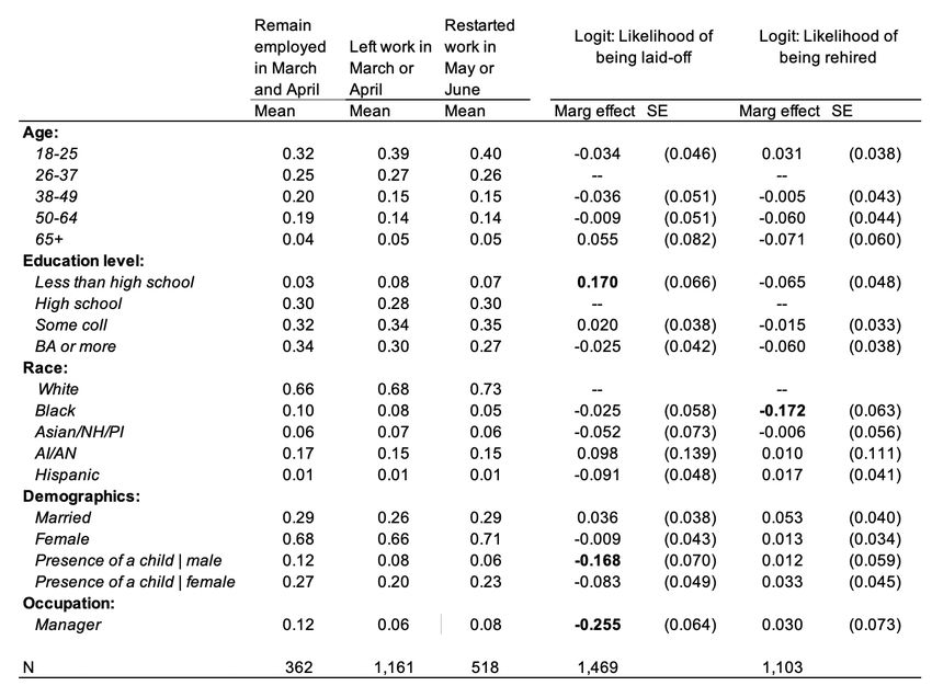
allows us to identify workers who were employed in March but not in April, or who were out of
work in April but re-employed in May.2

To ensure comparability over time, the labor force status questions in the CPS are maintained
unchanged from month to month. However, these questions were not designed for a pandemic. In
ordinary times, people without jobs are counted as unemployed only if they are available for work
and actively engaged in job search, so someone who would like a job but is not actively looking
due to shelter-in-place rules would be counted as out of the labor force. Similarly, the coding
structure is not designed to measure workers who are sheltering at home due to public health
orders, individualize quarantines, or school closures. Consequently, beginning in March, CPS
surveyors were given special instructions (Bureau of Labor Statistics 2020c): people who had jobs
but did not work at all during the reference week as a result of quarantine or self-isolation were to
be coded as out of work due to “own illness, injury, or medical problem,” while those who said
that they had not worked “because of the coronavirus” were to be coded as unemployed on layoff.
Interviewers were also instructed to code as on temporary layoff people without jobs who expected
to be recalled but did not know when, a break from ordinary rules that limit the category to those
who expect to be recalled within six months. Despite this guidance, many interviewers seem not
to have followed these rules, and unusually large shares of workers were classified as employed
but not at work for “other reasons,” while the share coded as out of the labor force also rose. As
we discuss below, if the misclassified workers are counted as unemployed on temporary layoff, as
the BLS commissioner suggests (BLS 2020a), the unemployment rate was notably higher in the
spring than the official rate.

BLS added several new questions to the May CPS to better probe job loss due to the pandemic
(BLS 2020b). At this writing, results from these questions are not yet available.

2
  The CPS is conducted via a combination of telephone and in-person interviews. In-person interviews were
suspended and two call centers were closed mid-way through data collection for the March survey, to avoid virus
transmission. Although the Census Bureau attempted to conduct the surveys by telephone, with surveyors working
from home, the response rate in March was about ten percentage points lower than in preceding months, and
continued to fall in subsequent months. While this may have impacted the accuracy of the survey, BLS’s internal
controls indicate that data quality is up to the agency’s standards.
                                                                                                                  4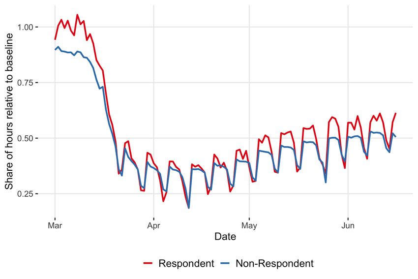
A last issue with the CPS concerns seasonal adjustment. Neither multiplicative nor additive
seasonal adjustment procedures are appropriate to an unprecedented situation. All CPS statistics
that we report here are not seasonally adjusted.

We use two other traditional sources: the monthly Current Employment Statistics survey of
employers, the source of official employment counts, and weekly unemployment insurance claims
reports, compiled by the Department of Labor.

We supplement the official data sources with daily data from a private firm, Homebase, which
provides scheduling and time clock software to tens of thousands of small businesses that employ
hundreds of thousands of workers across the U.S. and Canada. The time clock component of the
Homebase software measures the exact hours worked each day for each hourly employee at the
client firms. Homebase has generously made these data available to interested academic
researchers. We use them to construct measures of hours worked at the employer-worker-day level.
Employers are identified by their industry and location.

Homebase’s customer base is disproportionately composed of small firms in food and drink
services, retail, and other sectors that disproportionately employ hourly workers. The data exclude
most salaried employees, firms who do not require this type of time clock software for their
operations, and larger firms who would use their own software for this purpose. Consequently,
insights derived from the Homebase data should be viewed as relevant to hourly workers in small-
sized businesses, primarily in food services and retail, rather than to the labor market at large.
While not representative of the US labor market, the Homebase subpopulation is however highly
relevant to the current moment as the pandemic seems to have disproportionately affected the
industries that form the Homebase clientele.

When analyzing the Homebase data, we focus on U.S.-based firms that were already Homebase
clients before the onset of the pandemic. We separate Homebase clients into separate units for each
industry, state, and metropolitan statistical area (MSA) in which the client operates. We refer to
these as “firms,” and use them as the unit of analysis. We define a base period as the two weeks

                                                                                                 5
from January 19 to February 1, and we limit our attention to firms that had at least 80 total hours
worked, across all hourly workers, in this base period.3

We aggregate hours across all firms and workers in the sample in each day or week, sometimes
segmenting by state or industry or worker characteristics. We scale hours in each day or week as
a fraction of total hours worked (sometimes by state or industry or worker characteristics) in the
base period. In daily analyses, we divide by average hours for the same day of the week in the base
period; in weekly analyses, we divide by average weekly hours in the base period.

We consider a firm to have shut down if in any week (Sunday-Saturday) it had zero hours reported
by all of its workers. We do not observe work among salaried employees, so it is possible that
some firms that appear to us to have shut down are continuing to operate without hourly workers.
We consider a firm to have reopened if, following a shut down, it again appears with positive
hours. At reopened firms, we consider a worker to be a pre-existing employee if he or she had
hours with the firm before it shut down, and a new employee otherwise.

Appendix A presents summary statistics for the full Homebase sample. As noted earlier, Homebase
clients are disproportionately small firms. The median firm has full-time-equivalent employment
(of hourly workers) under 5; 80% have 10 or fewer (Appendix Figure A1). Nearly half of
Homebase clients are in the food & drink industry, and another 15% are in retail (Appendix Figure
A2). Homebase firms are also somewhat disproportionately concentrated in the West relative to
the Northeast and Midwest (Appendix Figure A3).

We supplement the Homebase data with information from a survey that Homebase allowed us to
conduct of the users of its software (i.e., of workers at client firms). Survey invitations were sent
via e-mail, starting May 1, to all individuals who were users of the software from February 2020
onwards. We use survey responses received by May 26, matched to the administrative records for
the same workers.

We limit the analysis of the survey data to those survey respondents that were represented in our
primary Homebase sample. We further restrict the analysis to workers with positive hours worked

3
  We exclude from all analyses any individual observations with more than 20 reported hours in a single day. We
also exclude firms in Vermont, which had fewer than 50 sample units among Homebase clients.
                                                                                                                  6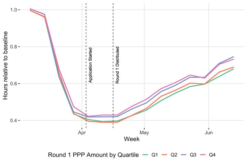
in our base period and who have worked for only one firm using the Homebase software since
January 19, 2020. Among the roughly 430,000 workers meeting this description, approximately
1,500 (0.3%) responded to our survey.4 Appendix Table B1 presents summaries of key survey
measures.

Despite the very low response rate, Appendix Table B2 shows that the survey respondents are
roughly representative of the population of Homebase workers that were active in our base period
and associated with a firm in our sample on the (limited set of) dimensions we can compare them
on. In particular, survey respondents broadly match the Homebase population in terms of their
distribution across Census division, industry, and employer size. However, survey respondents are
somewhat positively selected on hours worked at the Homebase employer (Appendix Figure B1)
and hence may be more representative of the “regular” workforce at these employers. Whereas the
average Homebase worker had about 10% fewer hours in early March than in the base period in
January, survey respondents saw no drop off in hours by this point.

As seen in Appendix Table B1, about 67 percent of survey respondents are female. Survey
respondents are young, with 37 percent of the sample between 18 and 25 years of age and another
27 percent between 26 and 37 years of age. A majority (55 percent) are single, and only 31 percent
have children. Two-thirds of survey respondents are white, while only 9 percent are Black, 16
percent are Hispanic, and 6 percent are Asian. More than 40 percent of survey respondents report
annual household income in 2019 below $25,000. The modal education in the sample is a two-
year college degree or some college (34 percent); 24 percent of respondents have a bachelor’s
degree and another 29 percent are high school graduates. The modal self-reported hourly wage
rate in this sample is $10-$12.50 (27 percent of survey respondents), with another 15 percent
earning between $7.50 and $10 per hour and another 20 percent between $12.50 and $15.00 per
hour; only 4 percent report hourly wages of $25 or more.

III.       Overview of the labor market collapse

Panel A of Figure 1 shows the unemployment rate and the employment-population ratio, as
reported in the official monthly employment reports from the Bureau of Labor Statistics. The labor

4
    We will update this analysis as more survey responses arrive.
                                                                                                7
market gradually strengthened from 2010 through early 2020. The unemployment rate has in
recent years been below the pre-Great Recession level, though the employment-population ratio
has not recovered its earlier peak, reflecting in part an aging population. However, things took a
sharp turn in spring 2020: The unemployment rate (not seasonally adjusted) spiked by 10.6
percentage points between February and April, reaching 14.4%, while the employment rate fell by
over 9 percentage points over the same period. These two-month changes were roughly 50% larger
than the cumulative changes in the respective series in the Great Recession, which took over two
years to unfold. Both unemployment and employment recovered a small amount in May, but
remain in unprecedented territory.

Table 1 tabulates the CPS microdata for the population age 18-64 across various labor market
states. The share employed at work fell by 14.4 percentage points between February and April.
The ranks of the unemployed more than tripled, from 2.9% to 10.4% (expressed as a share of the
population, rather than of the labor force), between February and April. Finally, the labor force
non-participation rate grew by 3.6 percentage points. Table 1 also shows that all of the categories
that grew in April shrunk somewhat in May, as the labor market recovered a bit.

As noted in Section II, the usual labor market categories are not well suited to measure a population
under shelter-in-place, and the BLS believes that the official unemployment rate has understated
the amount of joblessness. Additional rows in Table 1 show ways that the existing categories failed
to capture the decline in work during the pandemic. The increase in measured unemployment was
entirely driven by increases in the number of workers on layoff, who expected to be recalled to
their former positions; the share who were looking for new jobs shrunk slightly. This is a stark
contrast from past downturns. Prior to this year, temporary layoffs were thought to be a historical
phenomenon, of much lower significance in recent recessions than in the past. The share of the
unemployed who were on temporary layoff has never previously exceeded 30 percent, but rose to
nearly 80 percent in April.

The share who were employed but not at work grew by 3.3 percentage points, all driven by the
“other reasons” category. BLS believes much or all of the increase in this category is people who
should have been counted as on temporary layoff; if they are re-classified that way, the
unemployment rate in April rises from 14.4% to 19.2% (BLS 2020c). Similarly, a large share of

                                                                                                   8
the new nonparticipants said that they wanted jobs but were not actively looking for work or were
not available to take jobs. It seems likely that many of these were kept out of work by the pandemic
and would otherwise have been counted as unemployed. If they are included as well, the adjusted
unemployment rate rises well above 20%.
Monthly statistics are inadequate to understanding the rapidity of the labor market collapse. Panel
B of Figure 1 uses the Homebase data to show how employment at the subset of firms represented
in these data evolved on a daily basis. Reported in the Figure are total daily hours worked across
all firms in the Homebase sample, as a fraction of average total hours worked on the same day of
the week in the January 19 to February 1 base period. The total hours worked at Homebase firms
fell by approximately 60% between the beginning and end of March, with the bulk of this decline
in the second and third weeks of the month -- largely after the CPS reference week. The largest
single daily drop was on March 17, when hours, expressed as a percentage of baseline, fell by 12.9
percentage points from the previous day. The nadir seems to have been around the second week
of April. Hours have grown slowly and steadily since then. They made up perhaps one-third of the
lost ground by the May CPS reference week, and by the most recent data have recovered about
halfway to their beginning-of-March level.
Also apparent in Figure 1.B are clear day-of-week effects: Homebase employment is lower on
weekends than on weekdays since the onset of the crisis. Recall that the Homebase data are
normalized relative to the same day of the week in the baseline period, so if hours fell
proportionally on all days of the week we would not see this pattern. Evidently, Homebase firms
have reduced hours by more on weekends than on weekdays. This could reflect businesses
reducing to skeleton hours, all on weekdays, or perhaps disproportionate hours reductions or
shutdowns of customer-facing businesses with high weekend shares.
Another source of near-real-time information about the labor market is unemployment insurance
claims, shown in Figure 2. Initial claims spiked to unprecedented levels the week of March 21,
continued to grow through early April, and have gradually fallen since, though they remain several
multiples of pre-recession levels and even above the pre-2020 historical record. Over the twelve
weeks since March 14, over 40 million initial claims were filed.
9There were extensive reports of processing delays in the unemployment insurance system in March
and April, and it was not clear whether the ongoing high claims reflected ongoing layoffs or
backlogs of applicants who had been laid off in March but had been unable to file claims
immediately due to system congestion. The Homebase data suggest that processing delays may
not have badly distorted the time pattern; UI initial claims reached their peak just about the same
time that Homebase hours reached their nadir, and have been falling since as hours have recovered.
Figure 2 also shows continuing claims. After March 27, when the CARES Act was passed, we add
to claims under the regular UI program claims for new Pandemic Unemployment Assistance
(PUA) benefits for independent contractors and others who do not qualify for regular benefits and
claims for Pandemic Emergency Unemployment Compensation (PEUC), for those who have
exhausted their regular benefits. Continuing claims rose steadily through April and have fallen
only slowly since then, with nearly 30 million claims filed the last week of May. One puzzle of
recent months is that the number of unemployment insurance claimants has exceeded the number
of people counted as unemployed. This may be partially explained, however, by the prevalence of
misclassification in the CPS; expanded measures of unemployment are closer to or larger than the
number of UI claims. In the Homebase survey data, 41% of those who reported being furloughed,
laid off, or absent from work said that they had applied for unemployment benefits.
Hedin, Schnorr, and von Wachter (2020) have used administrative records from the California
unemployment insurance system to explore the characteristics of unemployment insurance
applicants. They find that over 90% of new claimants in late March reported that they expected to
be recalled to their prior jobs, up from around 40% in February. The share expecting recalls has
gradually declined since late March, to around 70% at the end of May, but this nevertheless
indicates that many of the job losses may not be permanent, and is consistent with the increase in
temporary layoffs measured by the CPS.
IV. Who are the unemployed? Who are the rehired?
A. Industry
Figure 3 shows how uneven the labor market collapse was across industrial sectors. We use payroll
employment data from the Current Employment Survey, conducted by BLS, to measure the total
10number of jobs in each primary industry by month. The CES counts paid workers, so may include
workers who are not at work but continuing to draw paychecks.
Not surprisingly, the low-wage segment of the private service sector of the economy experienced
the largest drop in employment. In the leisure and hospitality sector, which includes restaurants
and hotels, employment fell by about half between March and April. Other services, which include
repair and maintenance services, personal and laundry services, and services to private households,
were the second most impacted, with April employment numbers less than 80% of where they
stood in January. Workers employed in retail trade were also disproportionately exposed to the
COVID-19 shock, with nearly 15% of retail jobs lost in April.
Appendix Figure C1 shows the change in the number of workers by industry in the CPS. Patterns
are similar, with the largest job losses in the hospitality and other services industries. We also
examine patterns for hourly workers, a proxy for the sectors represented in Homebase data. We
find little evidence that the industry patterns of job loss differ dramatically for hourly and non-
hourly workers.
This sector composition of the COVID-19 crisis stands in contrast with that of the Great Recession
induced by the financial crisis in the late 2000s. Figure 4 compares the two-month decline in
employment from February to April 2020 with the cumulative decline between November 2007
and January 2010. It shows that this year we lost about 50% more jobs in total than in the whole
of the Great Recession, and that the industrial composition was quite different. The largest declines
in employment between November 2007 and January 2010 were in construction and durable goods
manufacturing; in contrast, the low-wage segment of the private service sector was relatively
insulated from the Great Recession.
Figure 3 further shows that the partial recovery has also been uneven across industrial sectors. For
example, the construction sector had nearly regained the April employment losses by May. Also,
while manufacturing, wholesale trade, education and health and professional and business services
experienced smaller job losses in April, little if any of these job losses had been recouped by May.
11B. Firm closings and reopenings
An advantage of Homebase data over the CPS, beyond its daily availability, is that it enables us to
link workers to their employers. We use this link to separate the observed change in total hours
documented above (Panel B of Figure 1) into three channels: firm shutdowns, layoffs, and cuts in
hours. To do this, we define a firm as having fully shut down in a given week if the Homebase
data records zero employees clocking in at that firm during that week. Among firms that have not
shut down, we count the proportional change in the number of workers with positive hours in a
week, relative to the baseline, and attribute that share of baseline hours to layoffs. Last, we define
hours cuts as the reduction in average hours, relative to the baseline period, among workers still
employed at still operating firms.
One important caveat to this decomposition is what we refer to as a firm shutdown is a shutdown
of Homebase-measured employment. If firms employ workers that do not schedule their time using
Homebase and some of these workers remain employed, some of the hours losses that we attribute
to shutdowns may instead be properly attributed to layoffs at continuing firms. Another caveat is
that the "hours cut" category includes all workers with positive hours during a given week. Hours
losses from workers who stop working in the middle of a week will be counted as hours reductions
in that week and will then convert to layoffs or firm closures the following week.
With these caveats in mind, Figure 5 reports the percent change in hours each week since early
February attributable to these three forms of hours reductions. As shown above, hours worked at
Homebase firms fell by 60 percent between the baseline period of Jan 19-Feb 1 and the week of
April 5-11 and have been slowly and steadily recovering since, reaching about 70 percent of
baseline by the second week of June. Except for the very first week of the labor market collapse
(week of March 15-21),5 hours reductions as defined above have accounted for a very minor part
of the change in total hours at Homebase businesses. Instead, the decline in total hours came
primarily from firms that closed entirely and from reductions in the number of workers at
continuing firms. The latter accounted for a larger share than the former in March, but thereafter
5
We conjecture that the large role for hours reductions in this week is an artifact created by mid-week layoffs or
firm closings. Consistent with this, Appendix Figure C4 shows that the distribution of hours per worker fell in that
week but returned to normal the following week and has been quite stable through the year to date, other than
transitory declines in holiday weeks.
12the two have had about the same quantitative impact on “missing hours” throughout the rest of the
sample period.6
The Homebase data also allows us to zoom in on the (partial) recovery period and assess the
channels via which hours are being restored at businesses that had shutdown at the nadir of the
labor market collapse. Of the roughly 42,000 unique firms in our baseline sample, approximately
half shut down for at least one week by April 4. In Figure 6, we report the distribution of hours at
these businesses from the week of April 6-11 to the week of June 7-13, as a share of total baseline
hours at these businesses. The figure shows that about 60 percent of baseline hours are still missing
at these businesses in the most recent week. Two-thirds (40 percentage points) of these missing
hours are attributable to businesses that remain closed. Another third (20 percentage points) of
missing hours can be attributed to businesses that have reopened but are doing so at reduced scale.
Of the 40 percent of hours that have been collectively regained, a vast majority has been coming
from rehiring of workers that were previously employed at these businesses (prior to the
shutdown), with only a very small share of hours regained coming from new hires. However, the
share attributable to new hires has been slowly trending up over time. New hires comprised only
5 to 7 percent of those re-employed at reopened firms between early April and early May; as of
the week ending June 13, that share has risen to almost 18 percent. This suggests that while most
firm-worker matches at these firms have been maintained through the crisis, the stability of these
matches has become more and more precarious as the time between firm closure and re-opening
increases.7
The Homebase data also allows us to investigate which businesses were more likely to shut down
as well as take an early look into which firms are most likely to make it through the crisis. While
Homebase does not collect much data from their employer clients, three employer characteristics
can be tracked: size (defined as the employer’s total number of unique employees in the Jan 19-
Feb 1 base period), industry, and growth rate (which we define as the change in the number of
6
Appendix Figure C5 shows firm exits in 2018, 2019, and 2020, using a stricter definition that counts firms as
exiting only if they do not return by mid-June. In prior years, about 2 percent of firms exit Homebase each month. In
March 2020, about 15 percent exited. After early April, the exit rate was similar to prior years.
7
Appendix Figure C3 shows the share of hours worked each day that came from workers who were present in the
base period. This falls off over time due to normal turnover. The rate of decline is not as steep in 2020 as it was in
2018 and 2019, however, consistent with firms operating at reduced capacity but filling vacancies primarily from
those who were laid off earlier.
13employees between January 2019 and January 2020, divided by the average of the beginning and
end-point levels, a ratio that is bounded between -2 and 2).
Reported in Figure 7 are marginal effects from logit models on the likelihood of the firm shutting
down by April 4, and, for firms that did, on the likelihood of re-opening by mid-June, controlling
for state and industry fixed effects. We find that larger firms are much less likely to shut down
than smaller firms. Larger firms are also somewhat more likely to have re-opened by the second
week of June conditional on having shut down, though this is not statistically significant. Across
industries, the shutdown rate was highest in the beauty and personal care industry, while employers
in the retail and health care and fitness sectors, which were not particularly likely to shut down,
had somewhat larger re-opening odds.8 Most interesting though is how the likelihood of shutting
down and re-opening is predicted by employer growth rate in the January 2019 to January 2020
period. There is a close to monotonic relationship, with more vibrant businesses (as proxied for by
higher employment growth in the pre-COVID period) having both a lower likelihood of shutting
down and a higher likelihood of re-opening conditional on shutting-down. That is, it is the
businesses that were already struggling pre-COVID that have the highest odds of shutting down
during the peak of the COVID crisis and of remaining closed. Three possible explanations are that
businesses that were already struggling prior to COVID might have been particularly low on cash
and unable to withstand the shock (Bartik et al., 2020); that those businesses may also have been
de-prioritized by banks when they applied for PPP funding; or that the COVID crisis sped up the
pruning of some of less productive businesses in the economy (Barrera, Bloom, and Davis, 2020).
Worker-level job loss and re-hiring
We now turn to examine the relationship between worker characteristics and job loss within
sectors. The first three columns of Table 2 report characteristics of three groups of workers: those
who were employed in both March and April, those who were employed in March but not in April,
and those who were out of work in April but started work in May. The second group, who we refer
to as “job losers” or as “laid off” workers though we also include voluntary departures and those
who have jobs but are not at work, has higher shares of very young (under 25) and old (over 65)
8
Figure C2 compares job loss by industry in Homebase and CPS data, using a crosswalk created by Etienne Lalé to
assign CPS employment to Homebase industries. The alignment is not particularly close, which we attribute to the
difficulty of matching the specific industry composition of Homebase clients within broader sectors.
14workers than does the group of continuously employed workers. Job losers are notably less
educated and more likely to be non-white. They are also more female, less likely to be married,
and less likely to have managerial positions. The third group of job returners broadly resembles
the job losers, with the notable exception that it includes a smaller share of Black workers and
somewhat fewer women.
To further understand the determinants of leaving work in April and of starting work in May, we
estimate multivariate logit models that include all of these characteristics as predictors, along with
fixed effects for states and major industry groupings. Our first logit model includes all CPS
respondents who worked in March and takes as the outcome the absence of work in April, while
the second is estimated on those not working in April and takes work in May as the outcome.
Marginal effects are shown in the rightmost columns of Table 2, and shown graphically in Figure
8.
The analysis reveals systematic differences across socio-demographic groups in the likelihood of
having stopped work in April that mostly mirror the unconditional patterns. We see a strong U-
shaped pattern in age for job loss. Workers that are 65 years of age or more (16 to 24 years of age)
were 14 (8) percentage points more likely to exit work in April compared to otherwise similar
workers in the 25 to 34 age group. The education gradient also remains quite strong. Workers
without a high school degree were 10 percentage points more likely to have stopped working in
April than similar workers with college degrees. There are also systematic racial differences.
Black, Asian, and Hispanic workers were, respectively, 4.6, 5.2, and 1.6 percentage points more
likely to exit work in April relative to otherwise similar white workers. Finally, married individuals
were less likely to lose jobs and women were more likely to do so. Perhaps surprisingly, we do not
observe systematic differences based on parental status, for either men or women.
These inequities in the distribution of job loss were for the most part not offset by re-hiring in May.
In particular, older workers, Black and Asian workers, and single workers were more likely to lose
their jobs in April and, having done so, less likely to start work again in May. However, education
gradients in re-hiring were comparatively weak, with both more- and less-educated workers less
likely to return to work than high school graduates.
15In Appendix Table C1, we replicate the logit models for the subset of workers that were employed
in hospitality and retail trade in March, to more closely match the industrial composition of the
Homebase dataset.9 Many of the patterns uncovered in the full CPS sample remain. The biggest
differences are that in these sectors Black and Hispanic workers are not disproportionately affected
by job loss (though Black workers are less likely to be rehired in May), and both male and female
workers with young children are less likely to have returned to work in May than their peers with
older children.
To conduct similar analyses in Homebase data, we link the administrative records on hours worked
to our worker survey, which provides demographic information. We also collected additional
worker characteristics that are not available in the CPS, such as the hourly wage rate, workers’
expectations about the crisis (such as expectation to be recalled if laid off or furloughed),
information about the nature of communication between employer and worker at the time of job
separation (such as whether the employer told the worker he or she would be rehired), and more
general information about how workers, especially those that have lost employment, have been
financially coping through the crisis.
Figure 9 presents time series for hours worked across education (panel A) and wage (panel B)
groups. Panel A shows that the lowest education group (those without a high school degree) was
most negatively impacted by COVID-19, with hours as low as 10 percent of baseline at the trough,
but also experienced a somewhat larger recovery, back to nearly 50 percent of baseline hours by
early June. In contrast, the COVID-19 shock was less extreme in the highest education group
(master’s degree or more) but recovery since the trough has also been much more muted for that
group. Moreover, while the magnitudes differed across education groups, the timing of hours loss
and recovery was nearly identical. Patterns of impact by hourly wage broadly match those by
education: workers with hourly wages below $15 saw their hours decline much more steeply than
those with hourly wages above $15, but they also experienced a faster recovery.
Table 3 repeats the analyses of job loss and rehiring from Table 2 in the Homebase data. We again
present the marginal effects from our logit analyses graphically in Figure 10. We define layoff and
9
The CPS allows us to identify hourly workers only in their last month in the sample, making it impossible to
conduct our longitudinal analyses of job loss and hiring on the subsample of hourly workers.
16rehiring somewhat differently, thanks to the higher frequency data: A worker is counted as leaving
work if he or she worked in the base period in January but had at least one week with zero hours
between March 8 and April 25; then, for these workers, we classify as re-hired those who returned
to work and recorded positive hours at some point between April 18 and the end of our sample.
Note that we do not distinguish in these definitions between firms that closed entirely and workers
who were laid off from continuing firms, nor similarly between re-hires at reopening vs. continuing
firms. We define explanatory variables as similarly as possible to the CPS.
Perhaps unsurprisingly, given the small sample size, few of the estimated effects are statistically
significant. However a few patterns emerge. We see a much higher likelihood of layoff among
those without a high school degree and much lower likelihood among those in managerial
positions. We also see that men with children were relatively spared from layoffs. In addition, as
in the CPS data, Black workers are notably less likely to be rehired.
The Homebase data also allows us to study how the likelihoods of layoff and rehiring (conditional
on layoff) differ across workers at different wage levels, tenure lengths, and prior full-time status.10
We augment the logit models from Table 3 with these predictors, and present marginal effects in
Figure 11. Full-time workers are 21 percentage points less likely to be laid off than otherwise
similar part-time workers; full-time workers are also (marginally significantly) more likely to be
rehired. Controlling for other worker characteristics, we do not see statistically significant
differences by hourly wage rate or by length of tenure at the firm, except that the lowest wage
workers (who are likely to be tipped workers) are marginally significantly less likely to be rehired.
In addition, though it is not statistically significant, those who have been with their employers for
over a year were somewhat less likely to be laid off.
The survey data we collected also allow us to understand more fully the experiences and
expectations of the Homebase workers. Twenty-two percent of the sample reported having
experienced a layoff as because of COVID, while 34 percent report having been furloughed and
20 percent report hours reductions. Less than 10 percent report having made the decision to not
10
We classify workers who worked more than 20 hours per week during our base period in late January as full-time.
We use wages as recorded in the Homebase administrative data, to maximize the sample size.
17work or work less, with most of those saying it was to protect themselves or their family members
from exposure to the virus. Less than 10 percent of the workers whose hours and employment
status has been negatively impacted by COVID report being paid for any of the hours that they are
not working. Among these negatively impacted workers, nearly 60 percent report that their
employers encouraged them to file for unemployment insurance. This was notably higher (78%)
among laid-off workers than among furloughed workers (66%) or workers who experienced
reduced hours (35%). Fifty-four percent of workers that have been laid off report that their
employer has expressed a desire to hire them back. Among workers that have been negatively
impacted by COVID, only about a quarter report looking for work, with the modal reason for not
being looking for work being an expectation to being rehired; only 8 percent attribute their lack of
job search to financial disincentives to work. Among the people that expect to be rehired, the modal
expectation about rehire date is June 1 (32 percent), with the second most common expectation
being July 1 (27 percent).
Respondents were also asked if they would return to their employer if offered the opportunity.
Three quarters of respondents said they would go back. Job satisfaction with this employer is an
important correlate of the decision to go back if asked. For example, 80% of workers who said that
they strongly agreed with the statement “I liked my manager” would plan to go back if asked,
compared with 67% who only somewhat agreed with this statement. Also, 91% of workers who
strongly agreed with “I was satisfied with my wages” would plan to go back to their prior employer
if asked, compared to 67% who only somewhat agree with this statement.
In Figure 12, we assess how answers to some of these questions relate to the likelihood of being
rehired (defined as above). The marginal effects presented in Figure 12 are from three separate
logit models where the only additional controls are state and industry fixed effects. Workers who
believed it was likely they would be rehired were 17 percentage points more likely to have been
rehired relative to other workers in the same industry and state who believed a rehiring was
unlikely. Similarly, workers who had been told by their employers that they would rehired were
26 percentage points more likely to be rehired than those who had been told they would not be
rehired. Similarly, we also see that workers that were encouraged by their employer to file for
unemployment insurance were slightly less likely to be rehired, but the difference here is not
statistically significant. Together, these results indicate that workers had access to predictive
18information about the odds of a maintained firm-worker match that may have helped at least some
of them better manage through what was otherwise a period of massive disruption and uncertainty.
The converse of this, though, is that the workers who have not yet been rehired disproportionately
consist of those who never expected to be, making it less likely that further recovery will lead to
additional rehiring.
V. Evaluating non-pharmaceutical interventions
Many of the firm closures observed to date were closely coincident with state closure orders and
other non-pharmaceutical interventions, and policy has generally proceeded on the assumption that
many of these firms will reopen when these orders are lifted. It’s not evident, however, that firms
closed or remain closed only because of government policy. Closures reflected increased
awareness about the threat posed by COVID-19, and consumers, workers, and firms might have
responded to this information with or without government orders. As for reopening, many
businesses have been permanently damaged by their closure and may not reopen. Moreover,
insofar as consumer behavior rather than state orders is the binding constraint on demand for firm
services, the mere lifting of an order may not be enough to restore adequate demand.
In this section, we study the relationship between state labor market outcomes and so-called
“shelter-in-place” and “stay-at-home” orders (which we refer to collectively as “shut-down
orders”) that restrict the public and private facilities that people can visit to essential businesses
and public services. We focus on this type of intervention because it is both the most prominent of
the non-pharmaceutical interventions and the one that may have the largest direct effects on
economic activity. We test the importance of these government directives on firms’ hours choices,
as captured by the Homebase data. We use event study models, using both contrasts between states
that did and did not implement shut-down orders and variation in the timing of these orders to
identify the effect of orders on hours worked. We also estimate event studies of the effect of the
lifting of public health orders, which need not be symmetric to the effect of imposing them.
Stay-at-home and reopen orders are sourced directly from government websites. They most
commonly come from centralized lists of executive orders (see Illinois.gov 2020, for example),
but in some cases come from centralized lists of public health and COVID-related orders (e.g.,
New Mexico Department of Health 2020). We define a stay-at-home order as any order that
19requires residents to stay at home or shelter in place (timed to the announcement date). Orders that
include COVID-related guidelines, but do not require residents to shelter in place (e.g.,
coronavirus.utah.gov 2020), are not included. In states that had stay-at-home orders, we define
reopen orders as the first lifting of these restrictions (timed to the effective date). Figure 13 shows
the number of states with active shut-down orders between the start of March and the present.
California was the first state to impose a shut-down order, on March 19. The number of active
orders then rose quickly, reaching 44 in early April. It was stable for about three weeks, but then
began to decline as some states removed their orders in late April and early May. By June 1, only
Wisconsin still had an order in place.
Stay-at-home orders can reduce employment simply by prohibiting non-essential workers from
going to work. But they can also have indirect effects operating through consumer demand, which
may relate to public awareness of COVID-19, willingness of consumers to visit businesses, and
COVID-19 caseloads. Consequently, we supplement our event study analysis of hours data from
Homebase with data on these three outcomes. We measure public awareness using Google trends
data on state-level relative search intensity for “coronavirus” from January to early June 2020. We
normalize these to set the maximal value in California at 100, relying on Google’s normalization
of other states relative to California.11 Overall mobility is measured using SafeGraph data on visits
to public and private locations between January 19 and June 13, 2020, including only locations
that recorded positive visits during our base period, January 19-February 1. We normalize the raw
count of visits by the number of devices that SafeGraph sees on each day to control for the
differences in the count of visits related to SafeGraph’s ability to track devices, then rescale relative
to the base period. State-level daily COVID-19 case data comes from the database maintained by
USAFacts, a source cited by CDC, and is divided by 2019 state population.
We estimate event-study models of the effect of shut-down and re-opening orders on the four
outcomes described above: log hours worked (from Homebase), log SafeGraph visits, an index of
11
This follows the approach used by Goldsmith-Pinkham, Pancotti, and Sojourner (2020) in normalizing Google
search trends when predicting unemployment claims.
20COVID-19 related Google searches, and log COVID-19 cases.12,13 Each outcome is measured at
the state-by-day level. We regress each on full sets of state and date fixed effects and a series of
indicators for “event time” relative to the imposition or lifting of a shut-down order (estimated
separately). We normalize the event time effect to zero fourteen days before a shut-down order is
put in place and seven days before a reopening order. The shut-down model is estimated on data
from February 16 to April 19, while the order lifting model is estimated on data from April 6
through June 13.
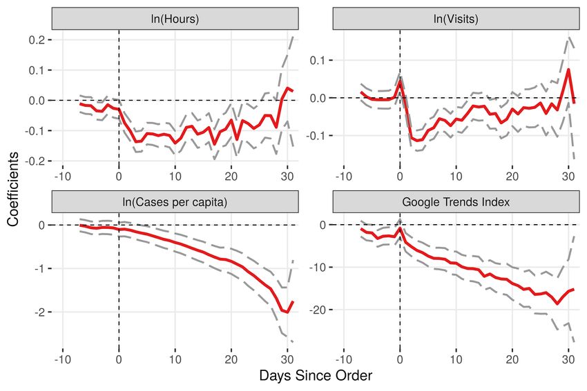
We report these results in Figure 14 (for shut-down orders) and 15 (for re-opening orders). In each
figure, Panel A reports results for our base specification, while Panel B reports results for an
additional specification that includes state-specific time trends. Each panel includes four sub-
panels, one for each of our outcomes. Starting with the estimates for the relationship between shut-
down orders and hours in Panel A of Figure 14, we see that hours worked began trending
downward a few days before shut-down orders began, but the trend accelerated in the days
immediately after the orders. The cumulative effect of the post-shutdown acceleration is to reduce
hours worked by about 10 to 15 log points two weeks after the order takes effect.
Turning to our measure of visits from SafeGraph, we see that there appears to be a very slight pre-
trend in visits, but a sharp, roughly 15 log point decline in visits after the shut-down orders are
implemented. Perhaps unsurprisingly given the lag in diagnoses and likely feedback from
diagnoses to orders, there is a strong pre-trend of cases with respect to orders, but little sign of an
immediate change when the order takes effect. Finally, turning to the last sub-panel on the
relationship between shut-down orders and Google searches about the coronavirus, we see a spike
in Google searches on the day of the implementation of the shut-down order, and then a decline
afterwards, possibly reflecting a decreased need to search for COVID-19 information once
information has initially been connected or decreased searches due to changing caseloads.
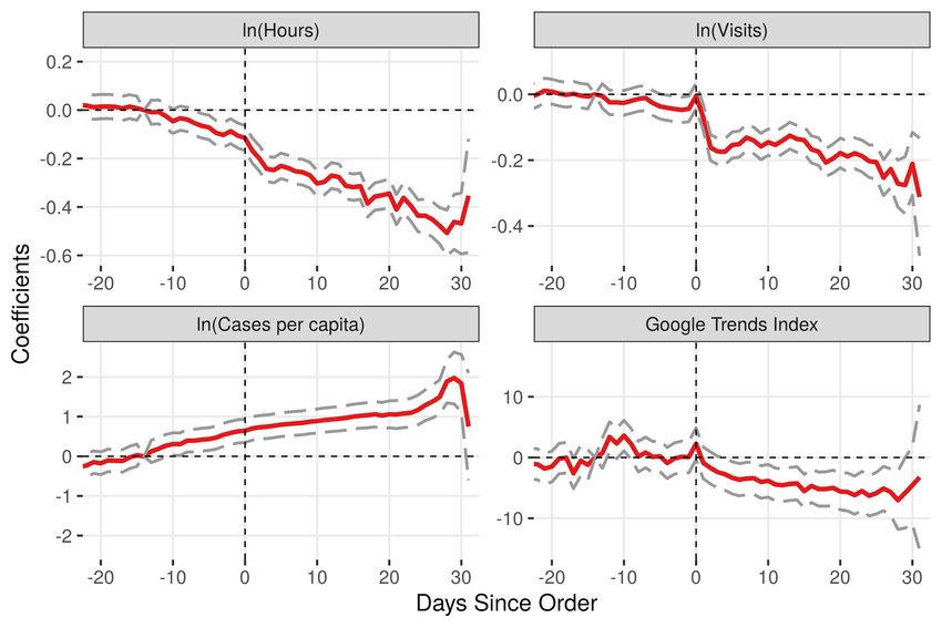
Panel B of Figure 14 reports event-study models that incorporate state-specific time-trends. These
models may be more robust to unobserved state heterogeneity that is correlated with treatment
12
We do not formally estimate the interaction of the different outcomes, but simply estimate reduced-form effects
of orders on each. For examples of studies that do examine interactions among outcomes, see Chernozhukov,
Kasahara, and Schrimpf (2020) and Allcott et al. (2020).
13
We use log((cases+1)/population) for to allow for zeroes.
21timing, but must be interpreted cautiously, given that they rely on the assumption that linear state-
specific trends are a good approximation for time trends in the absence of shut-down orders.14 That
being said, two interesting patterns present themselves in Panel B. First, both hours and visits
decline immediately after the shut-down orders and then slowly recover afterwards, returning to
the level of non-shut down states by about a month after the initial order. This may reflect
adjustment of firms or workers to the restrictions, reduced compliance, or reduced enforcement of
restrictions after they were put into place. Second, once state-specific trends are allowed for, there
does appear to be a gradual decline in caseloads per capita after shelter-in-place orders. Given the
lagged response of caseloads to changes in behavior, and the possibility that states implementing
shut-down orders also implemented other public interventions at the same time, more work is
necessary to fully understand the relationship between shut-down orders and caseloads. However,
these results are consistent with shut-down orders reducing cases per capita relative to states
without shut-down orders.
Figure 15 reports results from the corresponding specifications for re-opening orders. Focusing on
Panel B, which reports results with state-specific trends, we see that the effects of re-opening
orders broadly look like the mirror image of shut-down orders; hours and visits immediately rise,
while cases per capita slowly rise. The magnitudes are similar, although slightly smaller than those
for shut-down orders.
How should we interpret the magnitudes of the estimates in Figures 14 and 15? One way to think
about them is to compare the estimates of the effects of shelter-in-place to the calendar date effects
from the same specifications, which reflect other determinants of the outcomes that are common
to all states. Figure 16 reports the calendar date effects for each of our four outcomes from the
shut-down and reopening specifications reported in Figures 14A and 15A, respectively. The red
line reports the date effects from the shut-down model, covering February 16 to April 19, and the
blue line reports date effects from the re-opening model, which uses data from April 6 to June 13.
14
We have also estimated weighted event studies (Ben-Michael, Feller, and Rothstein 2019) that rely on matching
to identify control states with similar counterfactual trends. While traditional difference-in-differences and event
study models can be poorly behaved in the presence of heterogeneous treatment effects (Goodman-Bacon and
Marcus 2020; Callaway and Sant’Anna 2019), weighted event studies are not subject to this problem.
22We include both lines for the period from April 6 to 19 where the periods overlap, and normalize
the reopen estimates to align with the layoff estimates on April 13.
As expected given the results in Section 1 above, the calendar date effects show extremely large
reductions in hours (about 75 log points at the weekend trough and about 60 log points on
weekdays) and visits in mid-March, and rising cases per capita over time. These large changes
contrast with the comparatively modest effects of shut-down and re-opening orders that we
estimated in Figures 14 and 15. For example, the estimated effect of shut-down orders on log hours
is about one-sixth as large as the pure calendar time effects, while the estimated effect of shut-
down orders on log visits is about one-eighth of the calendar time decline in visits. Combined,
these results imply that, at least in the short-run, shut-down and re-opening orders are only a
modest portion of the changes in labor markets and economic activity during the crisis; the overall
patterns have more to do with broader health and economic concerns affecting product demand
and labor supply rather than with shut-down or re-opening orders themselves. This is consistent
with the relatively large effects we see on visits to businesses in Figures 15 and 16.
Two caveats are important to keep in mind when interpreting our finding that shut-down and re-
opening orders play only a modest role in the labor market effects of COVID-19. First, shut-down
orders may have spillover effects on other states not captured in our model. In particular, the first
shut-down orders may have played a role in signalling the seriousness and potential risk associated
with COVID-19, even if subsequent shut-down orders had more muted effects.
Second, over longer time horizons, the effects of shut-down orders on social distancing and
caseloads may result in larger labor market effects than we estimate here. For example, the slow
rebound of hours worked in Figure 14, Panel B may in part be due to reduced caseloads making
people more comfortable engaging in economic activity. Explorations of these more complicated
medium- and long-run interactions of shut-down orders, labor market activity, social distancing,
and caseloads is beyond the scope of our analysis here. Several papers, including Chernozhukov,
Kasahara, and Schrimpf (2020) and Allcott et al. (2020) have investigated these interactions by
combining treatment effect estimates like those here with epidemiological and economic models
that specify the relationships among our outcomes to estimate how the full system responds over
time to shut-down orders.
23You can also read