Genomics Tutorial 2019 - Instructors
←
→
Page content transcription
If your browser does not render page correctly, please read the page content below
Genomics Tutorial 2019.
Instructors:
● Josie Paris & the Workshop Team!
● Konrad Paszkiewicz in absentia (don’t worry he’s not dead).
Important Notes
username: genomics
password: see the whiteboard
Objectives:
Part 1: Short Read Genomics: An Introduction
● Understand how short reads are generated.
● Understand paired-end reads
● See possible sources of errors
● Learn about adaptors
Part 2: QC, Alignment and Variant Calling
● Interpret FASTQ quality metrics
● Remove poor quality data
● Trim adaptor/contaminant sequences from FASTQ data
● Count the number of reads before and after trimming and quality control
● Align reads to a reference sequence to form a SAM file (Sequence AlignMent file) using
BWA
● Convert the SAM file to BAM format (Binary AlignMent format)
● Identify and select high quality SNPs and Indels using SAMtools
● Identify missing or truncated genes with respect to the reference genome
● Identify SNPs which overlap with known coding regions
Part 3: Assembly of Unmapped Reads
● Extract reads which do not map to the reference sequence
● Assemble these reads de novo using SPAdes
● Generate summary statistics for the assembly
● Identify potential genes within the assembly
● Search for matches within the NCBI database via BLAST and against the Pfam database
1 of 88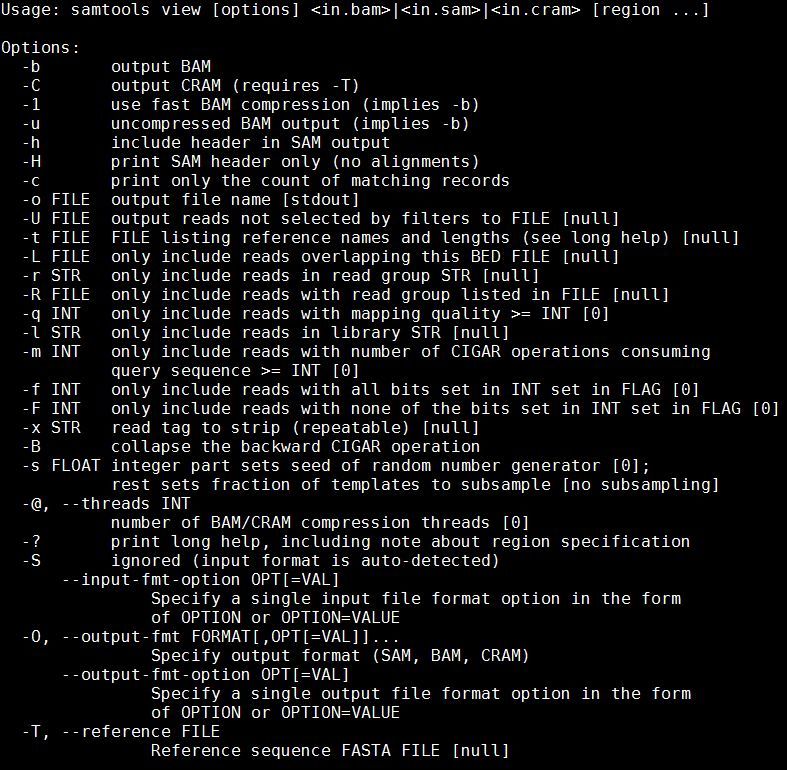
●   Visualize the taxonomic distribution of BLAST hits
    ●   Perform gene prediction and annotation using RAST

Part 4: De-novo Assembly Using Short Reads
    ●   Perform QC and adaptor-trim Illumina reads.
    ●   Assemble these reads de novo using SPAdes
    ●   Generate summary statistics for the assembly
    ●   Understand how to incorporate long PacBio reads into the assembly.
    ●   Identify open reading frames within the assembly
    ●   Search for matches within the NCBI database via BLAST and against the Pfam database
    ●   Visualize species distribution of potential matches

                                                                                      2 of 88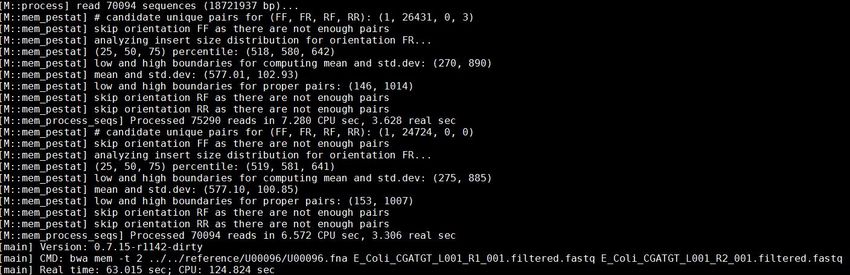
Table of Contents
Instructors:                                                                                       1

Important Notes                                                                                    1

Objectives:                                                                                        1
   Part 1: Short Read Genomics: An Introduction                                                    1
   Part 2: QC, Alignment and Variant Calling                                                       1
   Part 3: Assembly of Unmapped Reads                                                              1
   Part 4: De-novo Assembly Using Short Reads                                                      2

Part 1: Short Read Genomics: An Introduction                                                       5
   Introduction                                                                                    5
   Principles of Illumina-based Sequencing                                                         6
   DNA Library Preparation                                                                         7
   Sequencing                                                                                      8
   Base-calling                                                                                   10
   What are paired-end reads and why are they necessary?                                          11
   Inherent Sources of Error                                                                      13
       Frequency Cross-talk and Normalisation Errors                                              13
       Phasing/Pre-phasing                                                                        14
   Reads Containing Adaptors                                                                      14

Part 2: QC, Alignment and Variant Calling                                                         15
   Introduction                                                                                   15
   Quality Control                                                                                15
   Quality scores                                                                                 15
   FASTQ Format                                                                                   16
   Quality control – Evaluating the Quality of Illumina Data                                      17
   Task 1                                                                                         17
       Quality Scores                                                                             19
       Per tile Sequence Quality                                                                  21
       Per-base Sequence Content:                                                                 21
       Sequence Duplication Levels:                                                               22
       Overrepresented Sequences                                                                  23
   Task 2                                                                                         24
   We can perform a quick check (although this by no means guarantees) that the sequences in read
   1 and read 2 are in the same order by checking the ends of the two files and making sure that the
   headers are the same.                                                                           25
   Aligning Illumina Data to a Reference Sequence                                                 26
       Sequencing Error                                                                           26
       PCR Duplication                                                                            26

                                                                                              3 of 88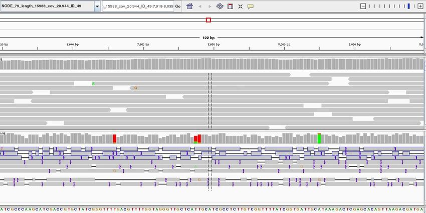
Indexing a Reference Genome                                                              27
   Task 3: Generating an index file from the reference sequence                             27
   Task 4: Aligning Reads to the Indexed Reference Sequence                                 29
   Task 9: Convert SAM to BAM File                                                          32
   Task 5: Sort BAM File                                                                    34
   Task 6: Remove Suspected PCR Duplicates                                                  34
   Task 7: Index the BAM File                                                               35
   Task 8: Obtain Mapping Statistics                                                        35
   Task 9: Cleaning up                                                                      36
   Task 10: QualiMap                                                                        37
   Task 11: Load the Integrative Genomics Viewer                                            39
   Task 12a: Import the E.coli U00096 Reference Genome to IGV                               40
   Task 12b: Load the BAM File                                                              42
   SNPs and Indels                                                                          45
   Task 13: Read about the Alignment Display Format                                         45
   Task 14a: Manually Identify a Region Without any Reads Mapping.                          45
   Task 14b: Manually Identify a Region Containing Repetitive Sequences.                    48
   Task 15: Identify SNPs and Indels Manually                                               48
      Example: Identifying Variants Manually                                                48
          Region U00096.3:2,108,392-2,133,153                                               49
          Region U00096.3:3,662,049-3,663,291                                               49
          Regions U00096.3:4,296,332-4,296,428                                              52
          Region U00096.3:565,965-566,489                                                   53
   Recap: SNP/Indel Identification                                                          53
   Automated Analyses                                                                       53
   Automated Variant Calling                                                                53
   Task 16: Identify SNPs and Indels using Automated Variant Callers                        53
   Task 23: Compare the Variants Found using this Method to Those You Found in the Manual
   Section                                                                                  57
      Quickly Locating Genes which are Missing Compared to the Reference                    57

Part 3: Assembly of Unmapped Reads                                                          58
   Introduction                                                                             58
   Extraction and QC of Unmapped Reads                                                      58
      Task 1: Extract the Unmapped Reads                                                    58
      Task 2                                                                                59
      Task 3: Evaluate QC of Unmapped Reads                                                 59
   De-novo Assembly                                                                         59
      Task 4: Learn More About de novo Assemblers                                           59
      Task 5: Generate the Assembly                                                         60
          params.txt                                                                        61

                                                                                        4 of 88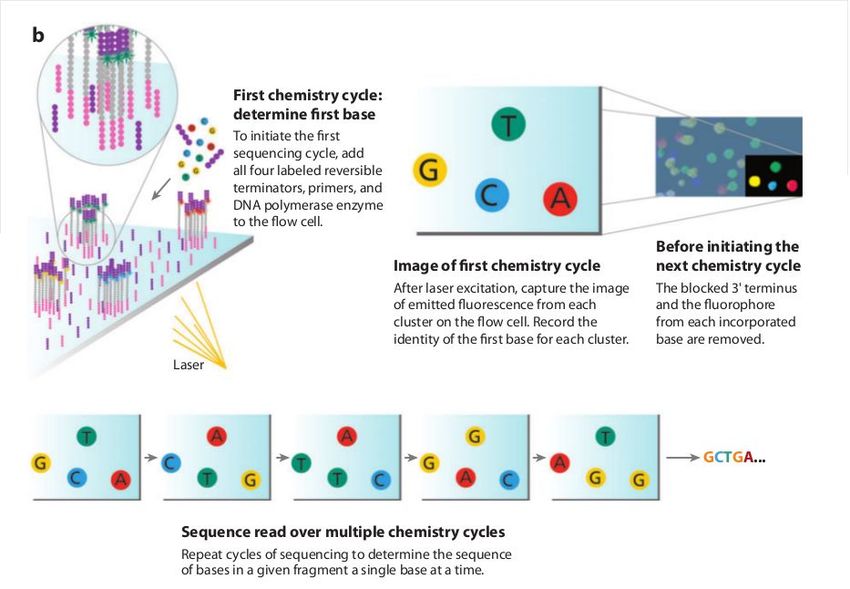
contigs.fasta                                                                           62
          scaffolds.fasta                                                                         62
          assembly_graph.fastg                                                                    62
       Task 6: Assessment of the Assembly                                                         62
   Analysing the de novo Assembled Reads                                                          63
       Task 7: Search Contigs against NCBI non-redundant Database                                 64
       Task 8: Obtain Open Reading Frames                                                         66
       Task 9: Search Open Reading Frames against NCBI non-redundant Database                     67
       Task 10: Review the BLAST Format                                                           68
   Additional Checks                                                                              69
       Task 11: Check that the Contigs do not Appear in the Reference Sequence                    69
       Task 12: Run Open Reading Frames Through pfam_scan                                         69

Part 4 De novo Assembly Using Short Reads                                                         71
   Introduction                                                                                   71
       Task 1: Start the Assembly                                                                 72
          Assembly Theory                                                                         72
       Task 2: Checking the Assembly                                                              76
       Task 3: Map Reads Back to Assembly                                                         77
       Task 4: View Assembly in IGV                                                               80
   Annotation of de novo Assembled Contigs                                                        83
       Task 5: Obtain Open Reading Frames                                                         83
   Hybrid de novo Assembly                                                                        83
       Task 7: QC the Data                                                                        84
       Task 8: Illumina Only Assembly                                                             85
       Task 9: Create Hybrid Assembly                                                             86
       Task 10: Align Reads Back to Reference                                                     87
   Summary                                                                                        90

Concluding Remarks                                                                                90

Part 1: Short Read Genomics: An Introduction

   1. Introduction
        Welcome to the genomics tutorial! Generating large amounts of data in biology is easy
these days. In little more than a fortnight we can generate more data than the entire human
genome project generated in over a decade of work. Making biological sense out of that data,
understanding its limitations and how the analysis algorithms work is now the major challenge for
researchers. The aim of this workshop is to take you through an example project. On the way, you
will learn how to evaluate the quality of data as provided by a sequencing facility, how to align the
data against a known and annotated reference genome and how to perform a de-novo assembly.
In addition you will also learn how to compare results between different samples.

                                                                                              5 of 88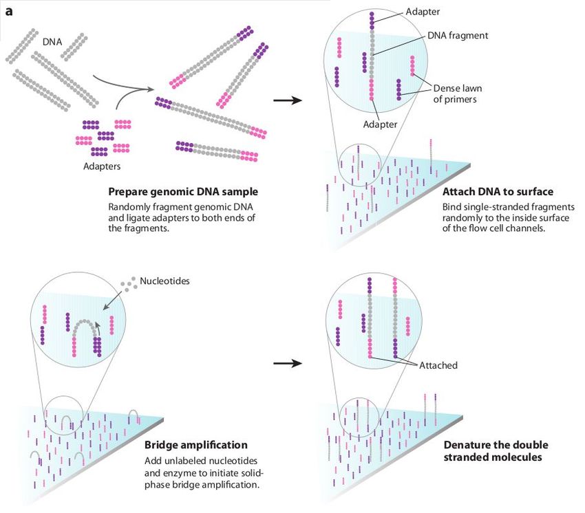
This workshop is broken into 4 parts. You should feel free to take as long as you like on each part.
It is much more important that you have a thorough understanding of each part, rather than try to
race through the entire workshop material.
The four parts are:
1. Short Read Introduction
2. Remapping a strain of E.coli to a reference sequence
3. Assembly of unmapped reads
4. Complete de-novo assembly of all reads
For this tutorial we will assume little background knowledge, except for a basic familiarity with the
Linux operating system and the cloud. We will cover the basics of how genomic DNA libraries are
generated and sequenced, and the principles behind short read paired-end sequencing. We will
look at why data can vary in quality, why adaptor sequences need to be filtered out and how to
quality control data. You may well do similar tasks in other tutorials at this workshop, especially
quality control and assembly techniques, this is good practice!
Then we will take the plunge and align the filtered reads to a reference genome, call variants and
compare them against the published genome to identify missing, truncated or altered genes. This will
involve the use of a publicly available set of bacterial E.coli Illumina reads and reference genome.
In parts 3 and 4 we will look at how one can identify novel sequences which are not present in the
reference genome.
A word on notation. If you see something like this:
cd ~/genomics_tutorial/reference_sequence
It means, type the highlighted text into your terminal. Please type the text, using all the tricks (e.g. tab
completion) that you have learnt in the Unix tutorial. Copying and pasting will sometimes not work with
certain characters and can cause errors. Also, please keep an eye for underscores!
Principles of Illumina-based Sequencing
There are several sequencers currently on the market. These include PacBio, MinION and the
various Illumina platforms (HiSeq, NextSeq, NovaSeq, MiSeq etc). Other (now obsolescent) platforms
included Life Tech SoLID and Roche 454 and many more are likely to appear in the future!
Regardless of the sequencer, all of these rely on making hundreds of thousands of clonal copies of a
fragment of DNA and sequencing the ensemble of fragments using DNA polymerase or in the case of
the SOLiD via ligation. This is simply because the detectors (basically souped-up digital cameras),
cannot detect fluorescence (Illumina, SolID, 454) or pH changes (Ion Torrent) from a single molecule.
The 'third-generation' Pacific Biosciences SMRT (Single Molecule Real Time) RSII and Sequel
sequencers are able to detect fluorescence from a single molecule of DNA. However, the machines
6 of 88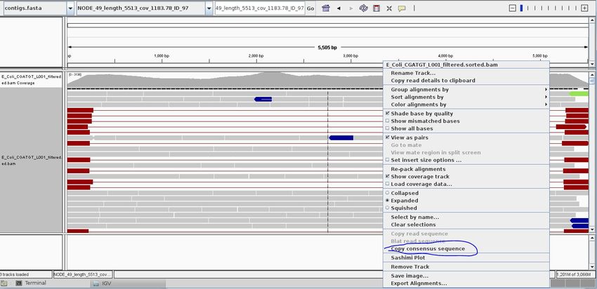
are very large (the RSII is almost 2 tons) and produces less than a tenth of the data of an Illumina
MiSeq run and for long reads >10kb error rates are generally around 10-12%. The Oxford Nanopore
MinION is another ‘third-generation’ single-molecule system which measures changes in electrical
current through a Nanopore as a single molecule is ratcheted through it. Although error rates are also
high (5-10%), and per-base costs are higher, the technology has improved rapidly and will probably
replace second generation systems over the next few years.
We will mainly look at the Illumina sequencing pipeline here, but the basic principles apply to other
second-generation sequencers. If you would like further details on other platforms then we
recommend reading: Mardis ER. Next-generation DNA sequencing methods. Annual Reviews
Genomics Hum Genet 2008; 9 :387–402.
A typical sequencing run would begin with the user supplying 1ng-1ug of genomic DNA to a
sequencing facility along with quality control information in the form of an automated electrophoresis
output (e.g. Agilent Bioanalyser/Tapestation trace) or gel image and quantification information.
DNA Library Preparation
For most sequencing applications, paired-end libraries are generated. Genomic DNA is
sheared into 300-500bp fragments (usually via sonication) and size-selected accordingly. Ends are
repaired and an overhanging adenine base is added, after which oligonucleotide adaptors are ligated.
In many cases the adaptors contain unique DNA sequences of 6-12bp which can be used to identify
the sample if they are 'multiplexed' together for sequencing. This type of sequencing is used
extensively when sequencing small genomes such as those of bacteria because it lowers the overall
per-genome cost.
7 of 88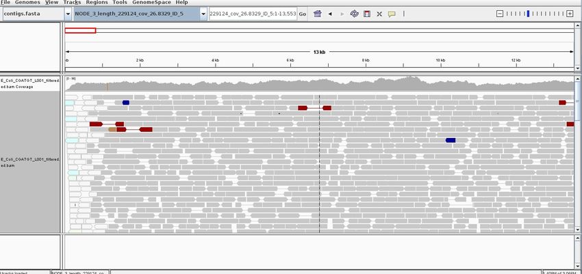
A) Steps a through e explain the main steps in Illumina sample preparation: a) the initial genomic
DNA, b) fragmentation of genomic DNA into 500bp fragments, c) end repair, d) addition of A bases to
the fragment ends and e) ligation of the adaptors to the fragments.
B) Overview of the automated the size selection protocol: The first precipitation discards fragments
larger than the desired interval. The second precipitation selects all fragments larger than the lower
boundary of the desired interval.
Borgström E, Lundin S, Lundeberg J, 2011 Large Scale Library Generation for High Throughput
Sequencing. PLoS ONE 6: e19119. doi:10.1371/journal.pone.0019119
Sequencing
(adapted from Margulis, E.R., reference below)
Once sufficient libraries have been prepared, the task is to amplify single strands of DNA to
form monoclonal clusters. The single molecule amplification step for the Illumina HiSeq 2500 starts
with an Illumina-specific adapter library and takes place on the oligo-derivatized surface of a flow cell,
and is performed by an automated device called a cBot Cluster Station. The flow cell is either a 2 or
8-channel sealed glass microfabricated device that allows bridge amplification of fragments on its
surface, and uses DNA polymerase to produce multiple DNA copies, or clusters, that each represent
the single molecule that initiated the cluster amplification.
Separate or multiple libraries can be added to each of the eight channels, or the same library can be
used in all eight, or combinations thereof. Each cluster contains approximately one million copies of
the original fragment, which is sufficient for reporting incorporated bases at the required signal
intensity for detection during sequencing. The Illumina system utilizes a sequencing- by-synthesis
approach in which all four nucleotides are added simultaneously to the flow cell channels, along with
DNA polymerase, for incorporation into the oligo-primed cluster fragments (see figure below for
details). Specifically, the nucleotides carry a base-unique fluorescent label and the 3 -OH group is
chemically blocked such that each incorporation is a unique event. An imaging step follows each base
incorporation step, during which each flow cell lane is imaged in three 100-tile segments by the
instrument optics at a cluster density of 600,000-800,000 per mm2. After each imaging step, the 3'
blocking group is chemically removed to prepare each strand for the next incorporation by DNA
polymerase. This series of steps continues for a specific number of cycles, as determined by
user-defined instrument settings, which permits discrete read lengths of 40–300 bases. A base-calling
algorithm assigns sequences and associated quality values to each read and a quality checking
pipeline evaluates the Illumina data from each run.
The next figures summarise the process:
8 of 88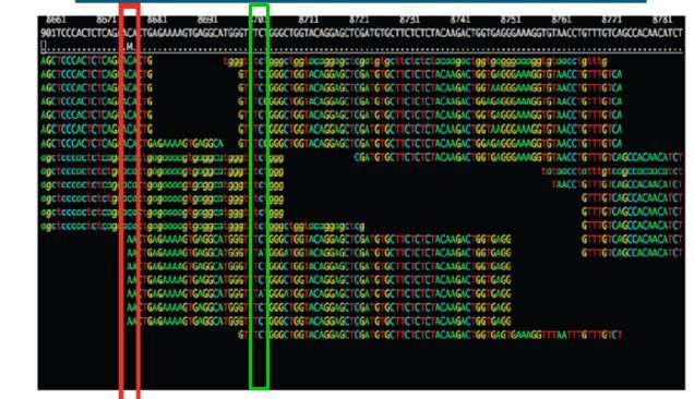
9 of 88
The Illumina sequencing-by-synthesis approach: Cluster strands created by bridge amplification are
primed and all four fluorescently labelled, 3 -OH blocked nucleotides are added to the flow cell with
DNA polymerase. The cluster strands are extended by one nucleotide. Following the incorporation
step, the unused nucleotides and DNA polymerase molecules are washed away, a scan buffer is
added to the flow cell, and the optics system scans each lane of the flow cell by imaging units called
tiles. Once imaging is completed, chemicals that affect cleavage of the fluorescent labels and the 3
-OH blocking groups are added to the flow cell, which prepares the cluster strands for another round of
fluorescent nucleotide incorporation. Next-Generation DNA Sequencing Methods Mardis, E.R. Annu.
Rev. Genomics Hum. Genet. 2008. 9:387–402

A short movie of the Illumina sequencing-by-synthesis approach can be found here:
https://www.youtube.com/watch?v=fCd6B5HRaZ8

Base-calling
        Base-calling involves evaluating the raw intensity values for each fluorophore and comparing
them to determine which base is actually present at a given position during a cycle. To call bases on
the Illumina platform, the positions of clusters need to be identified during the first few cycles. This is
because they are formed in random positions on the flowcell as the annealing process is stochastic.
        If there are too many clusters, the edges of the clusters will begin to merge and the image
analysis algorithms will not be able to distinguish one cluster from another (remember, the software is
dealing with upwards of half a million clusters per square millimeter – that's a lot of dots!).

                                                                                                  10 of 88
The above figure illustrates the principles of base-calling from cycles 1 to 9. If we focus on the
highlighted cluster, one can observe that the colour (wavelength) of light observed at each cycle
changes along with the brightness (intensity). This is due to the incorporation of complementary
ddNTPs containing fluorophores. So at cycle 1 we have a T base, at 2 a G base and so on. If the
colour or intensity is ambiguous the sequencer will mark it as an N. Other clusters are also visible in
the images; these will represent different monoclonal clusters with different sequences.
The base calling algorithms turn the raw intensity values into T,G,C,A or N base calls. There are a
variety of methods to do this and the one mentioned here is by no means the only one available, but it
is often used as the default method on the Illumina systems. Known as the 'Chastity filter' it will only
call a base if the intensity divided by the sum of the highest and second highest intensity is less than a
given threshold (usually 0.6). Otherwise the base is marked with an N. In addition the standard
Illumina pipeline will reject an entire read if two or more of these failures occur in the first 4 bases of a
read (it uses these cycles to determine the boundary of a cluster).
Note that these processes are carried out at the sequencing facility and you will not need to
perform any of these tasks under normal circumstances. They are explained here as useful
background information.
What are paired-end reads and why are they necessary?
Paired-end sequencing is a remarkably simple and powerful modification to the standard
sequencing protocol. It is nearly always worth obtaining paired-end reads if performing genomic
sequencing. Typically sequencers of any type are only able to sequence a portion of DNA (e.g. 100bp
11 of 88in the case of Illumina) before the fidelity of the enzyme and de-phasing of clusters (see later) increase
the error rate beyond tolerable levels. As a result, on the Illumina system, a fragment which is 500bp
long will only have the first 100bp sequenced.
If the size selection is tight enough and you know that nearly all the fragments are close to 500bp long,
you can repeat the sequencing reaction from the other end of the fragment. This will yield two reads
for each DNA fragment separated by a known distance. In the figure below the dashed regions
represent the complete DNA fragment and the solid lines the regions we are able to sequence:
Read 1
100bp
In the diagram below you can see a description of the nomenclature used when talking about paired
end reads
The added information gained by knowing the distance between the two reads can be invaluable for
spanning repetitive regions. In the figure below, the light coloured regions indicate repetitive sections
of DNA. If a read contains only repetitive DNA, an alignment algorithm will be able to map the read to
many locations in a reference genome. However, with paired-end reads, there is a greater chance that
12 of 88at least one of the two reads will map to a unique region of DNA. In this way one of the reads can be
used to anchor the other read in the pair and help resolve the repetitive region. Paired-end reads are
often used when performing de-novo genome sequencing (i.e. when a reference is not available to
align against) because they enable contiguous regions of DNA to be ordered, or when characterizing
variants such as large insertions or deletions.
Other forms of paired-end sequencing with much larger distances (e.g. 10kb) are possible with so
called 'mate-pair' libraries. These are usually used in specific projects to help order contigs in de-novo
sequencing projects. We will not cover them here, but the principles behind them are similar.
Inherent Sources of Error
No measurement is without a certain degree of error. This is true in sequencing. As such there
is a finite probability that a base will not be called correctly. There are several possible sources:
Frequency Cross-talk and Normalisation Errors
When reading an A base, a small amount of C will also be measured due to frequency overlap and
vice-versa. Similarly with G and T bases. Additionally, from the figure below, it should be clear that the
extent to which the dyes fluoresce differs. As such it is necessary to normalize the intensities. This
normalisation process can also introduce errors.
13 of 88Frequency response curve for A and C dyes
(Intensity y-axis and frequency on the x-axis)
Phasing/Pre-phasing
This occurs when a strand of DNA lags or leads the other DNA strands within a cluster. This
introduces additional background noise into the signal and reduces the intensity of the true base. In
the example below we have a cluster with 7 strands of DNA (very small, but this is just an example).
Five strands are on a C-base, whilst 1 is lagging behind (called phasing) on a G base and the
remaining strand is running ahead of the pack (confusingly called pre-phasing) on an A base. As such
the C signal will be reduced and A and G boosted for the rest of the sequencing run. Too much
phasing or pre-phasing (i.e. > 15-20%) usually causes problems for the base calling algorithm and
result in clusters being filtered out.
Other issues:
● Biases introduced by sample preparation – your sequencing is only as good as your
experimental design and DNA extraction. Also, remember that sometimes samples will be
put through several cycles of PCR before sequencing (unless they are PCR-free libraries).
This also introduces a potential source of bias.
● High AT or GC content sequences – this reduces the complexity of the sequence and
can result in higher error rates.
● Homopolymeric sequences – long stretches of a single base can make it difficult to
determine phasing and pre-phasing rates. This can introduce errors in determining the
precise length of a hompolymeric stretch of sequence. (This much more of a problem on
the old 454 and Ion Torrent than Illumina platforms but still worth bearing in mind).
Especially if you encounter indels which have been called in homopolymeric tracts.
● Some motifs can cause loops and other steric clashes.
14 of 88 akamura et al, Sequence-specific error profile of Illumina sequencers Nuc. Acid Res. first
See N
published online May 16, 2011 doi:10.1093/nar/gkr344
Reads Containing Adaptors
Some reads will contain adaptor sequences after sequencing, usually at the end of the read.
This is usually because of short sample DNA fragments, which result in the polymerase reading into
the adaptor region. Occasionally this can also happen because of mis-priming. It is important to
remove or trim sequences containing these reads as the adaptor sequences can prevent reads
mapping to a reference sequence and will adversely affect de-novo assembly.
Part 2: QC, Alignment and Variant Calling
Introduction
hich was sequenced at
In this section of the workshop we will be analysing a strain of E.coli w
the Exeter Sequencing Service. It is closely related to the K-12 substrain MG1655
(http://www.ncbi.nlm.nih.gov/nuccore/U00096). We want to obtain a list of single nucleotide
polymorphisms (SNPs), insertions/deletions (indels) and any genes which have been deleted.
Quality Control
In this section of the workshop we will be learning about evaluating the quality of an Illumina
MiSeq sequencing run. The process described here can be used with any FASTQ formatted file from
any platform (e.g. Illumina, PacBio etc).
Sequencers produce vast quantities of data. A single Illumina MiSeq lane can produce up to 15
Gigabases (Gbp) of data. However, the error rates of these platforms are 10-100x higher than Sanger
sequencing. They also have very different error profiles. Unlike Sanger sequencing, where the most
reliable sequences tend to be in the middle, NGS platforms tend to be most reliable near the
beginning of each read.
Quality control usually involves:
● Calculating the number of reads before quality control
● Calculating GC content, identifying overrepresented sequences
● Remove or trim reads containing adaptor sequences
● Remove or trim reads containing low quality bases
● Calculating the number of reads after quality control
● Rechecking GC content, identifying overrepresented sequences
Quality control is necessary because:
● CPU time required for alignment and assembly is reduced
15 of 88● Data storage requirements are reduced
● Reduce potential for bias in variant calling and/or de-novo assembly
Quality scores
To account for the possible errors and provide an estimate of confidence in a given base-call,
the Illumina sequencing pipeline assigns a quality score to each base called. Nowadays, all quality
scores are calculated using the Phred scale (Ewing B, Green P: Basecalling of automated sequencer traces
enome Research 8:186-194 (1998)). Each base call has an associated
using phred. II. Error probabilities. G
base call quality which estimates chance that the base call is incorrect.
Q10 = 1 in 10 chance of incorrect base call
Q20 = 1 in 100 chance of incorrect base call
Q30 = 1 in 1000 chance of incorrect base call
Q40 = 1 in 10,000 chance of incorrect base call
For most Illumina runs you should see quality scores between Q20 and Q40.
Note that these as only estimates of base-quality based on calibration runs performed by the
manufacturer against a sample of known sequence with (typically) a GC content of 50%. Extreme
GC biases and/or particular motifs or homopolymers can cause the quality scores to become
unreliable. Accurate base qualities are an essential part in ensuring variant calls are correct. As a
rough and ready rule we generally assume that with Illumina data anything less than Q20 is not useful
data and should be excluded.
Once you understand the FASTQ format try to work out what is happening to the quality scores here
and why:
FASTQ Format
A FASTQ entry consists of 4 lines
1. A header line beginning with '@' containing information about the name of the sequencer, and
the position at which the originating cluster was located and whether it passed purity filters.
2. The DNA sequence of the read
3. A header line or line beginning with just '+'
4. Quality scores for each base encoded in ASCII format
16 of 88To reduce storage requirements, the FASTQ quality scores are stored as single characters and
converted to numbers by obtaining the ASCII quality score and subtracting either 33 or 64. For
example, the above FASTQ file is Sanger formatted and the character ‘!’ has an ASCII value of 33.
Therefore the corresponding base would have a Phred quality score of 33-33=Q0 (i.e. totally
unreliable). On the other hand a base with a quality score denoted by ‘@’ which has an ASCII value
of 64 would have a Phred quality score of 64-33=Q31 (i.e. less than 1/1000 chance of being incorrect).
Just to confuse matters, there are several different methods of encoding quality scores in the ASCII
format. Although as of 2011, Illumina 1.8+/Phred+33 is used universally (and most likely, this will not
change in the future).
SSSSSSSSSSSSSSSSSSSSSSSSSSSSSSSSSSSSSSSSS............................................
.........
..........................XXXXXXXXXXXXXXXXXXXXXXXXXXXXXXXXXXXXXXXXXXXXXX.............
.........
...............................IIIIIIIIIIIIIIIIIIIIIIIIIIIIIIIIIIIIIIIII......................
.................................JJJJJJJJJJJJJJJJJJJJJJJJJJJJJJJJJJJJJJJ......................
LLLLLLLLLLLLLLLLLLLLLLLLLLLLLLLLLLLLLLLLLL....................................................
!"#$%&'()*+,-./0123456789:;?@ABCDEFGHIJKLMNOPQRSTUVWXYZ[\]^_`abcdefghijklmnopqrstuvwxyz{|}~
| | | | | |
33 59 64 73 104 126
0........................26...31.......40
-5....0........9.............................40
0........9.............................40
3.....9.............................40
0.2......................26...31.........41
S Sanger- Phred+33, raw reads typically (0, 40)
X Solexa- Solexa+64, raw reads typically (-5, 40)
I -
Illumina 1.3+ Phred+64, raw reads typically (0, 40)
J -
Illumina 1.5+ Phred+64, raw reads typically (3, 40)
with 0=unused, 1=unused, 2=Read Segment Quality Control Indicator (bold)
(Note: See discussion above).
L - Illumina 1.8+ Phred+33, raw reads typically (0, 41)
Note that the latest Illumina CASAVA 1.8 pipeline (released June 2011), outputs in fastq-sanger rather
than Illumina 1.3+. Thus Illumina 1.3+ and other Illumina scoring metrics are unlikely to be
encountered if you are using Illumina sequencing data generated after July 2011.
Quality control – Evaluating the Quality of Illumina Data
The first task when one receives sequencing data is to evaluate its quality and determine
whether all the cash you have handed over was well-spent! To do this we will use the FastQC toolkit
(https://www.bioinformatics.babraham.ac.uk/projects/fastqc/). FastQC offers a graphical visualisation
of QC metrics, but does not have the ability to filter data.
17 of 88Task 1
Open a terminal window. From your home directory change into:
workshop_materials/genomics_tutorial/data/sequencing/ecoli_exeter/ directory and list the directory
contents, e.g.
cd ~/workshop_materials/genomics_tutorial/data/sequencing/ecoli_exeter/
ls -l
***Note that you will also see two other directories here as well: blast_precompute and
denovo_assembly. Don’t worry about these directories for now as we will come back to them later in
the tutorial.
For the purposes of this tutorial, we have already cleaned the data so you will see four files
Raw reads:
● read 1 (E_Coli_CGATGT_L001_R1_001.fastq)
● read 2 (E_Coli_CGATGT_L001_R2_001.fastq)
Cleaned reads:
● read 1 (E_Coli_CGATGT_L001_R1_001.filtered.fastq)
● read 2 (E_Coli_CGATGT_L001_R2_001.filtered.fastq)
These are paired-end data and so reads from the same pair can be identified because they will have
the same header. Many programs require that the read 1 and read 2 files have the reads in the same
order. We will look at the raw reads. To view the first few headers we can use the head and grep
commands:
head E_Coli_CGATGT_L001_R1_001.fastq | grep MISEQ
head E_Coli_CGATGT_L001_R2_001.fastq | grep MISEQ
The only difference in the headers for the two reads is the read number. Of course this is no guarantee
that all the headers in the file are consistent. To get some more confidence repeat the above
commands using 'tail' instead of 'head' to compare reads at the end of the files.
You can also check that there is an identical number of reads in each file using cat, grep and wc –l:
cat E_Coli_CGATGT_L001_R1_001.fastq | grep MISEQ | wc -l
18 of 88cat E_Coli_CGATGT_L001_R2_001.fastq | grep MISEQ | wc -l
Now, let's run the fastqc program on the data. Unlike the QC lab, we will open up a Graphical User
Interface (GUI) and load the data this way. To do this, run:
fastqc &
Load the E_Coli_CGATGT_L001_R1_001.fastq file from the
~/workshop_materials/genomics_tutorial/data/sequencing/ecoli_exeter directory.
The fastqc program performs a number of tests which determines whether a green tick (pass),
exclamation mark (warning), or red cross (fail) is displayed. However, it is important to realise that
fastqc has no knowledge of what your library is or should look like. All of its tests are based on a
completely random library with 50% GC content. Therefore if you have a sample which does not
match these assumptions, it may 'fail' the library. For example, if you have a high AT or high GC
organism it may fail the per sequence GC content. If you have any barcodes or low complexity
libraries (e.g. small RNA libraries) they may also fail some of the sequence complexity tests.
The bottom line is that you need to be aware of what your library is and whether what fastqc is
reporting makes sense for that type of library.
19 of 88In this case we have a number of errors and warnings which at first sight suggest there has been a
problem - but don't worry too much yet. Let's go through them in turn.
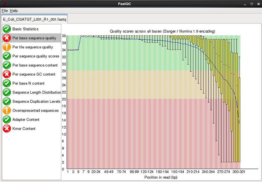
Quality Scores
This is one of the most important metrics. If the quality scores are poor, either the wrong
FASTQ encoding has been guessed by fastqc (see the title of the chart), or the data itself is poor
quality. This view shows an overview of the range of quality values across all bases at each position in
the FASTQ file. Generally anything with a median quality score greater than Q20 is regarded as
acceptable; anything above Q30 is regarded as 'good'. For more details, see the help documentation
in fastqc.
In this case this check is red - and it is true that the quality drops off at the end of the reads. It is
normal for read quality to get worse towards the end of the read. You can see that at 250 bases the
quality is still very good.
20 of 88Per tile Sequence Quality
This is a purely technical view on the sequencing run, it is more important for the team running
the sequencer. The sequencing flowcell is divided up into areas called cells. The colour of the tiles
indicate the read quality and you can see that the quality drops off in some cells faster than others.
This maybe because of the way the sample flowed over the flowcell or a mark or smear on the lens of
the optics.
Per-base Sequence Content:
For a completely randomly generated library with a GC content of 50% one expects that at any
given position within a read there will be a 25% chance of finding an A,C,T or G base. Here we can
see that our library satisfies these criteria, although there appears to be some minor bias at the
beginning of the read. This may be due to PCR duplicates during amplification or during library
preparation. It is unlikely that one will ever see a perfectly uniform distribution. See
http://sequencing.exeter.ac.uk/guide-to-your-data/quality-control/ f or examples of good vs bad runs as
well as the fastqc help for more details.
21 of 88Sequence Duplication Levels:
In a library that covers a whole genome uniformly most sequences will occur only once in the
final set. A low level of duplication may indicate a very high level of coverage of the target sequence,
but a high level of duplication is more likely to indicate some kind of enrichment bias (e.g. PCR
over-amplification).
This module counts the degree of duplication for every sequence in the set and creates a plot showing
the relative number of sequences with different degrees of duplication.
22 of 88Overrepresented Sequences
This checks for sequences that occur more frequently than expected in your data. It also
checks any sequences it finds against a small database of known sequences. In this case it has found
that a small number of reads 4000 out of 600000 appear to contain a sequence used in the
preparation for the library. A typical cause is that the original DNA was shorter than the length of the
read - so the sequencing overruns the actual DNA and runs in to the adaptors used to bind it to the
flowcell.
23 of 88There are other reports available:
Have a look at them and at what the author of FastQC has to say here:
https://www.bioinformatics.babraham.ac.uk/projects/fastqc/Help/3%20Analysis%20Modules/ or check
out their youtube tutorial video: https://www.youtube.com/watch?v=bz93ReOv87Y.
Remember the error and warning flags are his (albeit experienced) judgement of what typical data
should look like. It is up to you to use some initiative and understand whether what you are seeing is
typical for your dataset and how that might affect any analysis you are performing.
Task 2
Do the same for the raw read 2 as we have for raw read 1. Open fastqc and analyse the read 2 file.
Look at the various plots and metrics which are generated. How similar are they?
Also look at the cleaned reads. How do they differ? You should notice very little change (since
comparatively few reads were filtered). However, you should notice a significant improvement in
quality and the absence of adaptor sequences.
24 of 88We can perform a quick check (although this by no means guarantees) that the sequences in read 1
and read 2 are in the same order by checking the ends of the two files and making sure that the
headers are the same.
head E_Coli_CGATGT_L001_R1_001.filtered.fastq | grep MISEQ
head E_Coli_CGATGT_L001_R2_001.filtered.fastq | grep MISEQ
tail E_Coli_CGATGT_L001_R1_001.filtered.fastq | grep MISEQ
tail E_Coli_CGATGT_L001_R2_001.filtered.fastq | grep MISEQ
Check the number of reads in each filtered file. They should be the same. To do this use the grep
command to search for the number of times the header appears, e.g.
grep -c “MISEQ” E_Coli_CGATGT_L001_R1_001.filtered.fastq
Do the same for the E_Coli_CGATGT_L001_R2_001.filtered.fastq file.
Note: Typically when submitting raw Illumina data to NCBI or EBI you would submit unfiltered data, so
don't delete your original fastq files!
A note on quality control using MultiQC
MultiQC (https://multiqc.info/) is software which will aggregate reports (such as fastqc) across a whole
experiment. For example, it will aggregate fastqc reports for multiple samples. Say you have 1000
samples in an experiment, you’re not going to want to open 1000 tabs on an internet browser! MultiQC
supports many other QC softwares (such as outputs from qualimap, quast, bcftools). At the time of
writing (2019), MultiQC supports 72 commonly-used bioinformatics tools. Take a look!
A note on checking for contaminants:
A number of tools are available now which also enable to you to quickly search reads and assign them
to particular species or taxonomic groups. These can serve as a quick check to make sure your
samples or libraries are not contaminated with DNA from other sources. If you are performing a
de-novo assembly for example and unwittingly have DNA sequence present from multiple organisms,
you will risk poor results and chimeric contigs.
Some ‘contaminants’ can turn out to be inevitable by-products of sampling and DNA extraction. This is
often the case with algae or other symbionts. In addition, some groups have made some amazing
discoveries such as the discovery of a third symbiont (which turned out to be a yeast) in lichen.
http://science.sciencemag.org/content/353/6298/488.full
Some tools you can use to check the taxonomic classification of reads include:
● Kraken
25 of 88● Centrifuge
● Blobology
● Kaiju
● Blast (in conjunction with subsampling your reads) and Krona to plot results.
Blobtools is also a useful tool for quality control post assembly. Blobtools visualizes the GC content,
coverage, and taxonomic classification of assembled contigs to enable screening for potential
contaminants. You can read more about Blobtools here , but we won’t do either of these steps today.
Aligning Illumina Data to a Reference Sequence
Now that we have checked the quality of our raw data, we can begin to align the reads against
a reference sequence. In this way we can compare how the reference sequence and the strain we
have sequenced compare to one another.
To do this we will be using a program called BWA (Burrows Wheeler Aligner Li H. and Durbin R. (2009)
Fast and accurate short read alignment with Burrows-Wheeler Transform. Bioinformatics, 25:1754-60.). This
uses an algorithm called (unsurprisingly) Burrows Wheeler to rapidly map reads to the reference
genome. BWA also allows for a certain number of mismatches to account for variants which may be
present in strain 1 vs the reference genome. Unlike other alignment packages such as Bowtie (version
1) BWA allows for insertions or deletions as well. (Note, there is now a Bowtie2 tool that allows for insertions and
deletions, but we’ll continue to use BWA here). There are also a host of newer aligners such as minimap2
(https://github.com/lh3/minimap2) that allow for long-read sequencing and employ different algorithms.
In fact, Heng Li (creator of both BWA and minimap2) suggests that minimap2 is now superior,
although bwa is still recommended for short read genomic data. For information on this, please see
Heng Li’s post here: http://lh3.github.io/2018/04/02/minimap2-and-the-future-of-bwa
By mapping reads against a reference, what we mean is that we want to go from a FASTQ file listing
lots of reads, to another type of file (which we'll describe later) which lists the reads AND where/if it
maps against the reference genome. The figure below illustrates what we are trying to achieve here.
Along the top in grey is the reference sequence. The coloured sequences below indicate individual
sequences and how they map to the reference. If there is a real variant in a bacterial genome we
would expect that (nearly) all the reads would contain the variant at the relevant position rather than
the same base as the reference genome. Remember that error rates for any single read on second
generation platforms tend to be around 0.5-1%. Therefore a 300bp read is on average likely to contain
at 2-3 errors.
Let's look at 2 potential sources of artefacts.
Sequencing Error
The region highlighted in green on the right shows that most reads agree with the reference
sequence (i.e. C-base). However, 2 reads near the bottom show an A-base. In this situation we can
safely assume that the A-bases are due to a sequencing error rather than a genuine variant since the
26 of 88‘variant’ has only one read supporting it. If this occurred at a higher frequency however, we would
struggle to determine whether it was a genuine variant or an error.
PCR Duplication
The highlighted region in red on the left shows where there appears to be a variant. A C-base
is present in the reference and half the reads, whilst an A-base is present in a set of reads which all
start at the same position.
Is this a genuine difference or a sequencing or sample prep error? What do you think? If this was a
real sample, would you expect all the reads containing an A to start at the same location?
The answer is probably not. This 'SNP' is in fact probably an artefact of PCR duplication. I.e. the same
fragment of DNA has been replicated many times more than the average and happens to contain an
error at the first position. We can filter out such reads during alignment to the reference (see later).
Note that the entire region above seems to contain lots of PCR duplicates with reads starting at the
same location. In the case of the region highlighted in red, this will likely cause a false SNP call. The
area in green also contains PCR duplicates – the As at these positions are probably either sequencing
errors or errors introduced during PCR.
It's always important to think critically about any finding - don't assume that whatever bioinformatic
tools you are using are perfect. Or that you have used them perfectly.
27 of 88Indexing a Reference Genome
Before we can start aligning reads to a reference genome, the genome sequence needs to be
indexed. This means sorting the genome into easily searched chunks, a bit like an index in a book.
Task 3: Genera ting an index file from the reference sequence
Change directory to the reference directory:
cd ~/workshop_materials/genomics_tutorial/data/reference/U00096/
In this directory we have 2 files. U00096.fna is a FASTA file which contains the reference genome
sequence. The U00096.gff file contains the annotation for this genome. We will use this later.
First, let's looks at the bwa command itself. Type:
bwa
This should yield something like:
BWA is actually a suite of programs which all perform different functions. We are only going to use two
during this workshop, bwa index, bwa mem
If we type:
bwa index
28 of 88We can see more options for the bwa index command:
By default bwa index will use the IS algorithm to produce the index. This works well for most
genomes, but for very large ones (e.g. vertebrate) you may need to use bwtsw. For bacterial genomes
the default algorithm will work fine.
Now we will create a reference index for the genome using BWA:
bwa index U00096.fna
If you now list the directory contents, you will notice that the BWA index program has created a set of
new files. These are the index files BWA needs.
Task 4: Aligning Reads to the Indexed Reference Sequence
Now we can begin to align read 1 and read 2 to the reference genome. First of all change back
into the ~/workshop_materials/genomics_tutorial/data/sequencing/ecoli_exeter/ directory
and create a subdirectory to contain our remapping results.
cd ~/workshop_materials/genomics_tutorial/data/sequencing/ecoli_exeter/
mkdir remapping_to_reference
cd remapping_to_reference
We’ll use the ‘bwa mem’ alignment algorithm to map the reads to the target genome. Let's explore the
alignment options BWA MEM has to offer. Type:
bwa mem
29 of 88The basis format of the command is:
Usage: bwa mem [options]
We can see that we need to provide BWA with a FASTQ files containing the raw reads (denoted by
and ) to align to a reference file (listed as ). There are also a number of
options. The most important are the maximum number of differences in the seed (-k i.e. the first 32 bp
of the sequence vs the reference), the number of processors the program should use (your machine
has 2 processors).
Our reference sequence is in
~/workshop_materials/genomics_tutorial/data/reference/U00096/U00096.fna
Our filtered reads in
~/workshop_materials/genomics_tutorial/data/sequencing/ecoli_exeter/E_Coli_CGATGT_
L001_R1_001.filtered.fastq
~/workshop_materials/genomics_tutorial/data/sequencing/ecoli_exeter/E_Coli_CGATGT_
L001_R2_001.filtered.fastq
So to align our paired reads using processors and output to file
E_Coli_CGATGT_L001_filtered.sam:
type, all on one line:
30 of 88bwa mem -t 2
~/workshop_materials/genomics_tutorial/data/reference/U00096/U00096.fna
~/workshop_materials/genomics_tutorial/data/sequencing/ecoli_exeter/E_Coli_
CGATGT_L001_R1_001.filtered.fastq
~/workshop_materials/genomics_tutorial/data/sequencing/ecoli_exeter/E_Coli_
CGATGT_L001_R2_001.filtered.fastq > E_Coli_CGATGT_L001_filtered.sam
This will take about 5 minutes to complete.
There will be quite a lot of output but the end should look like:
31 of 88Viewing the alignment
Once the alignment is complete, list the directory contents and check that the alignment file is present.
ls -lh
Note: ls -lh outputs the size of the file in human readable format (780Mb in this case – yours may be
slightly different depending on the storage options you selected when you started the AMI)
The raw alignment is stored in what is called SAM format (Simple AlignMent format). It is in plain text
format and you can view it if you wish using the 'less' command. Do not try to open the whole file in a
text editor as you will likely run out of memory!
less E_Coli_CGATGT_L001_filtered.sam
Each alignment line has 11 mandatory fields for essential alignment information such as mapping
position, and a variable number of optional fields for flexible or aligner specific information. For further
details as to what each field means see https://en.wikipedia.org/wiki/SAM_(file_format) or
http://samtools.sourceforge.net/SAM1.pdf
Task 9: Convert SAM to BAM File
Before we can visualise the alignment however, we need to convert the SAM file to a BAM
(Binary AlignMent format) which can be read by most software analysis packages. To do this we will
use another suite of programs called samtools. Type:
samtools view
32 of 88We can see that we need to provide samtools view with a reference genome in FASTA format file (-T),
the -b and -S flags to say that the output should be in BAM format and the input in SAM, plus the
alignment file.
Remember our reference sequence is in:
~/workshop_materials/genomics_tutorial/data/reference/U00096/U00096.fna
Type (all on one line):
samtools view -bS -T
~/workshop_materials/genomics_tutorial/data/reference/U00096/U00096.fna
E_Coli_CGATGT_L001_filtered.sam > E_Coli_CGATGT_L001_filtered.bam
33 of 88This should take around 2 minutes. Note that for larger datasets you may wish to set multiple threads
as well with the --threads option.
ls -lh
It's always good to check that your files have processed correctly if something goes wrong it's better to
catch it immediately.
Note that the bam file is smaller than the sam file - this is to be expected as the binary format is more
efficient.
Task 5: Sort BAM File
Once this is complete we then need to sort the BAM file so that the reads are stored in the
order they appear along the chromosomes. We can do this using the samtools sort command. In this
instance, we will sort
samtools sort -n E_Coli_CGATGT_L001_filtered.bam -o
E_Coli_CGATGT_L001_filtered.sorted.bam
The -n option sorts the sam file by read name (which is needed below for samtools fixmate)
This will take another minute or so.
Task 6: Remove Suspected PCR Duplicates
Especially when using paired-end reads, samtools can do a reasonably good job of removing
potential PCR duplicates (see the first part of this workshop if you are unsure what this means).
Again, samtools has a great little command to do this called markdup. To run this tool, we will have to
generate some intermediate files (see Task 9 for cleaning these up afterwards), using other samtools
programs. At each stage of the process, we will document which tool has been run by appending the
name of the tool on the end of the file.
To run samtools markdup, you’ll first need to run samtools fixmate which fills in various coordinates
and flags from a name-sorted alignment (hence why used the -n option above)
On the command-line type:
samtools fixmate -m E_Coli_CGATGT_L001_filtered.sorted.bam
E_Coli_CGATGT_L001_filtered.sorted.fixmate.bam
And then sort the file again (this time without the -n option!), which will sort the file by genomic
coordinates.
34 of 88samtools sort E_Coli_CGATGT_L001_filtered.sorted.fixmate.bam -o
E_Coli_CGATGT_L001_filtered.sorted.fixmate.position.bam
Now we can run samtools markdup to remove PCR duplicates!
samtools markdup E_Coli_CGATGT_L001_filtered.sorted.fixmate.position.bam
E_Coli_CGATGT_L001_filtered.sorted.fixmate.position.markdup.bam
You may notice some warnings about inconsistent BAM file for pair - this is just a warning that a pair of
reads does not align together on the genome within the expected tolerance - it is normal to expect
some of these, and you can ignore.
Task 7: Index the BAM File
Most programs used to view BAM formatted data require an index file to locate the reads
mapping to a particular location quickly. You can think of this as an index in a book, telling you where
to go to find particular phrases or words. We'll use the samtools index command to do this.
Type:
samtools index
E_Coli_CGATGT_L001_filtered.sorted.fixmate.position.markdup.bam
We should obtain a .bai file (known as a BAM-index file).
Task 8: Obtain Mapping Statistics
Finally we can obtain some summary statistics.
samtools flagstat
E_Coli_CGATGT_L001_filtered.sorted.fixmate.position.markdup.bam >
mappingstats.txt
This should only take a few seconds. Once complete view the mappingstats.txt file using a text-editor
(e.g. gedit or nano) or the 'more' command.
35 of 88So here we can see we have 1269900 reads in total, none of which failed QC.
72.31% of reads mapped to the reference genome and 71.98% mapped with the expected 500-600bp
distance between them. 1414 reads could not have their read-pair mapped.
0 reads have mapped to a different chromosome than their pair (0 has a mapping quality > 5 – this is a
Phred scaled quality score much as we say in the FASTQ files). If there were any such reads they
would likely due to repetitive sequences
Task 9: Cleaning up
We have a number of leftover intermediate files which we can now remove to save space.
Type (all on one line):
rm E_Coli_CGATGT_L001_filtered.sam E_Coli_CGATGT_L001_filtered.sorted.bam
E_Coli_CGATGT_L001_filtered.sorted.fixmate.bam
E_Coli_CGATGT_L001_filtered.sorted.fixmate.position.bam
In case you get asked if you are sure to remove 4 arguments type in “yes” and hit enter.
You should now be left with the processed alignment file, the index file and the mapping stats.
Well done! You have now mapped, filtered and sorted your first whole genome data-set!
Let's take a look at it!
36 of 88Task 10: QualiMap
Qualimap (http://qualimap.bioinfo.cipf.es/) is a program that summarises the alignment in much
more detail than the mapping stats file we produced. It’s a technical tool which allows you to assess
the sequencing for any problems and biases in the sequencing and the alignment rather than a tool to
deduce biological features.
There are a few options to the program, We want to run bamqc. Type:
qualimap bamqc
to get some help on this command.
To get the report, first make sure you are in the directory:
~/workshop_materials/genomics_tutorial/data/sequencing/ecoli_exeter/remapping_to_r
eference
then run the command:
qualimap bamqc -outdir bamqc -bam
E_Coli_CGATGT_L001_filtered.sorted.fixmate.position.markdup.bam -gff
~/workshop_materials/genomics_tutorial/data/reference/U00096/U00096.gff
this creates a subfolder called bamqc
move into this directory and run
firefox qualimapReport.html
There is a lot in the report so just a few highlights:
37 of 88This shows the number of reads that 'cover' each section of the genome. The red line shows a rolling
average around 50x - this means that on average every part of the genome was sequenced 50X. It is
important to have sufficient depth of coverage in order to be confident that any features you find in
your data are real and not a result of sequencing errors.
What do you think the regions of low/zero coverage correspond to?
38 of 88The Insert Size Histogram displays the range of sizes of the DNA fragments. It shows how well your
DNA was size selected before sequencing. Note that the 'insert' refers to the DNA that was inserted
between the sequencing adaptors, so equates to the size range of the DNA that was used.
In this case we have 300 base pair paired end reads and our insert size varies around 600 bases - so
there should only be a small gap between the reads that was not sequenced.
Have a look at some of the other graphs produced.
Task 11: Load the Integrative Genomics Viewer
The Integrative Genome Viewer (IGV) is a tool developed by the Broad Institute for browsing
interactively the alignment data you produced. It has a wealth of features and we can only cover some
basics to get you started. Go to http://www.broadinstitute.org/igv/ to get more information.
In your terminal, type
igv.sh
39 of 88Or you can click the icon on the desktop.
IGV viewer should appear:
Notice that by default a human genome has been loaded.
Task 12a: Import the E.coli U00096 Reference Genome to IGV
By default IGV does not contain our reference genome. We'll need to import it.
Click on 'Genomes ->Create .genome file...'
40 of 88Enter the information above and click on ‘OK’ .
IGV will ask where it can save the genome file. Your home directory will be fine.
Click 'Save' again.
Note that the genome and the annotation have now been imported.
41 of 88Task 12b: Load the BAM File
Load the alignment file. Note that IGV requires the .bai index file to also be in the same directory.
Select File... and Load From File
Select the bam file and click open
Once loaded your screen should look similar to the following. Note that you can load more BAM files if
you wish to compare different samples or the results of different mapping programs.
42 of 88Select the chromosome U00096.3 if it is not already selected
Use the +/- keys to zoom in or use the zoom bar at the top right of the screen to zoom into
about 1-2kbases as above
Right click on the main area and select view as pairs
The gray graph at the top of the figure indicates the coverage of the genome:
The more reads mapping to a certain location, the higher the peak on the graph. You'll see a coloured
line of blue, green or red in this coverage plot if there are any SNPs (single-nucleotide polymorphisms)
present (there are none in the plot). If there are any regions in the genome which are not covered by
the reads, you will see these as gaps in the coverage graph. Sometimes these gaps are caused by
43 of 88repetitive regions; others are caused by genuine insertions/deletions in your new strain with respect to
the reference.
Below the coverage graph is a representation of each read pair as it is mapped to the genome. One
pair is highlighted.
This pair consists of 2 reads with a gap (there may be no gap if the reads overlap) Any areas of
mismatch either due to inconsistent distances between paired-end reads or due to differences
between the reference and the read are highlighted by a colour. The brighter (or less transparent) the
colour, the higher the base-calling quality is estimated to be. Differences in a single read are likely to
be sequencing errors. Differences consistent in all reads are likely to be mutations.
Hover over a read to get detailed information about the reads' alignment:
You don't need to understand every value, but compare this to the SAM format to get an idea of what
is there.
44 of 88SNPs and Indels
The following 3 tasks are open-ended. Please take your time with these. Read the examples
on the following page if you get stuck.
Task 13: Read about the Alignment Display Format
Visit http://www.broadinstitute.org/software/igv/AlignmentData
Task 14: Manually Identify a Region Without any Reads Mapping.
It can be quite difficult to find even with a very small genome. Zoom out as far as you can and
still see the reads. Use the coverage plot from QualiMap to try to find it. Are there genes associated?
Because of the way IGV handles BAM files, it will not display coverage information if you zoom out too
far. To get coverage information across the entire genome, regardless of how far you are zoomed out,
you’ll need to create a TDF file which contains a coverage information across windows of X number of
bases across the genome. You can do this within IGV:
Select Tools->Run igvtools:
Now load the BAM alignment file in the Input field and click Run:
45 of 88You can also read