Specimen-Based Modeling, Stopping Rules, and the Extinction of the Ivory-Billed Woodpecker
←
→
Page content transcription
If your browser does not render page correctly, please read the page content below
Contributed Paper

Specimen-Based Modeling, Stopping Rules, and
the Extinction of the Ivory-Billed Woodpecker
NICHOLAS J. GOTELLI,∗ ANNE CHAO,† ROBERT K. COLWELL,‡ WEN-HAN HWANG,§
AND GARY R. GRAVES#
∗
 Department of Biology, University of Vermont, Burlington, VT 05405, U.S.A., email ngotelli@uvm.edu
†Institute of Statistics, National Tsing Hua University, Hsin-Chu 30043, Taiwan
‡Department of Ecology and Evolutionary Biology, University of Connecticut, Storrs, CT 06269-3043, U.S.A.
§Department of Applied Mathematics, National Chung Hsing University, Tai-Chung 402, Taiwan
#Department of Vertebrate Zoology, MRC-116, National Museum of Natural History, Smithsonian Institution, PO Box 37012,
Washington, D.C. 20013-7012, U.S.A., and Center for Macroecology, Evolution, and Climate, University of Copenhagen, Denmark

Abstract: Assessing species survival status is an essential component of conservation programs. We devised
a new statistical method for estimating the probability of species persistence from the temporal sequence of
collection dates of museum specimens. To complement this approach, we developed quantitative stopping rules
for terminating the search for missing or allegedly extinct species. These stopping rules are based on survey
data for counts of co-occurring species that are encountered in the search for a target species. We illustrate
both these methods with a case study of the Ivory-billed Woodpecker ( Campephilus principalis), long assumed
to have become extinct in the United States in the 1950s, but reportedly rediscovered in 2004. We analyzed
the temporal pattern of the collection dates of 239 geo-referenced museum specimens collected throughout
the southeastern United States from 1853 to 1932 and estimated the probability of persistence in 2011 as
48                                                                                                   Specimen-Based Extinction Assessment

métodos con un estudio de caso de Campephilus principalis, considerada extinta en los Estados Unidos desde
la década de 1950, pero supuestamente redescubierta en 2004. Analizamos el patrón temporal de fechas de
colecta de 239 especı́menes de museo georeferenciados colectados en el sureste de Estados Unidos de 1853 a
1932 y estimamos que la probabilidad de persistencia en 2011 es < 6.4 × 10⁻⁵ , con una probable extinción
no posterior a 1980. De un análisis de datos de censos aviares (conteos de individuos) en 4 sitios en los que
realizaron búsquedas de C. principalis desde 2004, estimamos que cuando hay 1-3 especies no detectadas en
3 sitios (uno en Louisiana, Mississippi y Florida). En un cuarto sitio en el Rı́o Congaree (Carolina del Sur), no
hubo unidades simples (especies representadas por una observación) después de 15,500 conteos de individuos
de aves, lo cual indica que es poco probable que incremente el número de especies ya registradas (56) con
mayor esfuerzo de muestreo. Colectivamente, estos resultados sugieren que virtualmente no hay oportunidad
para que C. principalis exista actualmente en su rango de distribución histórica en el sureste de Estados
Unidos. Los resultados también sugieren que los recursos de conservación destinados a su redescubrimiento y
recuperación deberı́an ser asignados a otras especies. Los métodos que describimos para la estimación de las
fechas de extinción y la probabilidad de persistencia de especies generalmente son aplicables a otras especies
de las que se disponga de suficientes colecciones de museo y censos de campo.

Palabras Clave: Campephilus principalis, censos aviares, especı́menes de museo, estimación de la probabilidad
de extinción, estimadores de la riqueza de especies, reglas de decisión

Introduction                                                         (2009a, 2009b) used estimates of the probability of pres-
                                                                     ence after a number of consecutive absences as the basis
Increasing effort in conservation biology is being devoted           for decision making in light of trade-offs between the fi-
to the analysis of extinction risk (Sodhi et al. 2008) and           nancial cost of continued searching and the ecological
the search for rare, long unseen, or potentially extinct             benefit of confirmed eradication.
species (Eames et al. 2005). For many species, statisti-                Results of any method that assesses the probability of
cal methods offer a means to guide and assess these ef-              extinction hinge heavily on the quality of the data, which
forts. This paper introduces new statistical tools for this          can range from reliable physical evidence (such as actual
purpose that substantially extend the ability of existing            specimens or dated biological materials) to unconfirmed
methods (reviewed by Rivadeneira et al. 2009 and Vogel               visual sightings (McKelvey et al. 2008). Analyses that in-
et al. 2009) to maximize the use of available data sources.          corporate more liberal criteria for detection inevitably
   In practice, declaring a species extinct is rarely analo-         lead to estimates of more recent (or future) extinction
gous to a coroner’s certification of death. Instead, the as-         dates. If the confidence interval about these estimates
sessment of extinction requires a probabilistic statement            extends to include the present, the statistical analysis im-
(Elphick et al. 2010) because extinction is very difficult           plies that the species may be extant, even in the absence
to definitively establish (Diamond 1987). The search for             of recent occurrence records.
a putatively missing species routinely begins with a ret-               Rivadeneira et al. (2009) recently reviewed 7 exist-
rospective analysis of the temporal sequence of occur-               ing statistical methods used to estimate extinction dates
rence records, including both dated museum specimens                 and associated confidence intervals. All 7 methods treat
and field sightings. Imagine an idealized string of such             occurrence records as a binary sequence of presences
temporal records, perhaps derived from annual surveys                and absences and assume a stable population size fol-
for a species. If there were no failures to detect an ex-            lowed by sudden extinction. All but 2 methods poorly
tant species, the data would consist of an uninterrupted             predicted known dates of extinction in simulations that
string of ones (presences) until the date of extinction              modeled declining total detection probability (proba-
and thereafter a continued string of zeroes (absences)               bility of occurrence × probability of sampling). More-
after the extinction event.                                          over, both these possible exceptions (Roberts & Solow
   In reality, there are failures to detect an extant species,       2003; Solow & Roberts 2003) tended toward excessive
including historically rare species endemic to inaccessi-            type I error (i.e., an extant species is declared extinct)
ble places and formerly common, widespread species in                (Rivadeneira et al. 2009).
decline. Thus, empirical data of this form often consist                Collen et al. (2010) showed that, for declining popula-
of irregular sequences of ones and zeroes. The statistical           tions, the Roberts and Solow (2003) method (further dis-
challenge is to distinguish between a terminal string of             cussed by Solow [2005]) is prone to both type I and type
zeroes, ending in the present, that represents a probable            II errors (i.e., an extinct species is declared extant). In
extinction and one that more likely suggests nondetec-               some simulation scenarios, the Roberts and Solow (2003)
tion. In the related context of the intentional eradication          method tends to yield conservative confidence intervals
of invasive species, Regan et al. (2006) and Rout et al.             that are too wide. Solow (1993b) proposes nonstationary

Conservation Biology
Volume 26, No. 1, 2012
Gotelli et al. 49
Poisson models that assume, instead, that a population de- area once the probability of detecting a new species be-
clines before reaching extinction. However, these meth- comes very small.
ods have proven difficult to implement (Solow 2005). We analyzed museum specimen records and bird
On the basis of binary time series data for 27 possibly counts from contemporary censuses to illustrate the ap-
extinct bird populations, Vogel et al. (2009) endeavored plication of these methods to the case of the Ivory-billed
to assess the fit of such records to a series of underlying Woodpecker (Campephilus principalis), which is gen-
sampling distributions and were unable to reject the uni- erally assumed to have become extinct in southeast-
form distribution for presence–absence data over time. ern North America in the 1950s (Jackson 2004; Snyder
However, statistical power to discriminate among distri- et al. 2009), but was reportedly rediscovered in 2004
butions was low, and both the uniform distribution and (Fitzpatrick et al. 2005, Sibley et al. 2006). The last well-
2 declining distributions (truncated negative exponential documented population of this large, strikingly-patterned
and Pareto) offered a reasonable fit to the binary occur- woodpecker disappeared from northeastern Louisiana in
rence data. With this result in mind, Elphick et al. (2010; the mid-1940s (Jackson 2004; Snyder et al. 2009). Sight-
see also Roberts et al. 2010) applied Solow’s (1993a) sta- ings in subsequent decades were sporadic and uncon-
tionary Poisson method and Solow and Roberts’ (2003) firmed, and the Ivory-billed Woodpecker was generally
nonparametric method to estimate extinction dates for presumed extinct until the recent reports from Arkansas.
38 rare bird taxa on the basis of physical evidence and The video image recorded in the Cache River National
expert opinion. Wildlife Refuge in 2004 (Fitzpatrick et al. 2005) and a
In this paper, we propose a new statistical method for subsequent flurry of uncorroborated sightings captured
estimating extinction dates that does not assume popula- the public’s imagination, precipitated major, fully docu-
tion sizes are constant in the time periods before extinc- mented search efforts, and triggered recovery plans un-
tion and does not treat occurrence records as a binary der the U.S. Endangered Species Act (U.S. Fish & Wildlife
presence–absence sequence. Instead, our method takes Service 2009). However, the video evidence was soon
full advantage of counts of specimens (or other reliable disputed by independent researchers (Sibley et al. 2006;
occurrence records) recorded during specific time inter- Collinson 2007), who argue the images are of the simi-
vals (McCarthy 1998; Burgman et al. 2000). larly sized Pileated Woodpecker (Dryocopus pileatus).
Dated, georeferenced specimens, deposited in muse- Because of the symbolic importance of the Ivory-billed
ums and natural history collections around the world, Woodpecker and the potential economic impact of ac-
represent a rich source of data for conservation biologists tions mandated under the Endangered Species Act, we
(Burgman et al. 1995; McCarthy 1998; Pyke & Erhlich think it is essential to quantify the probability that it per-
2010) and are often the only source of information avail- sists and the probability of discovering it through ad-
able on past abundances and geographic distribution. ditional searches. We applied a statistical approach to
Museum specimen records correspond to distinct occur- answer 2 questions. First, on the basis of the tempo-
rence records of different individuals, which is often not ral distribution of museum specimens collected during
the case for visual sightings, photographic records, or the 19th and 20th centuries (Hahn 1963), what is the
other indirect signs of a species’ presence. Our method probability that the woodpecker survives in the 21st cen-
relates specimen records, in a simple way, to population tury? Second, given the investment in search efforts, since
sizes and provides estimates of the probability of occur- 2004, that have not resulted in an undisputed occurrence
rence in past or future time intervals. record, what is the probability that any additional species
Programs aimed at rediscovering possibly extinct will be found at the survey sites with further effort?
species (Roberts 2006) sometimes offer a second, and
relatively untapped, source of information for the statisti-
cal assessment of extinction that is independent of spec-
imen records. Rediscovery programs often use standard- Methods
ized sampling methods developed for species richness
Specimen-Based Analyses
inventories (e.g., Hamer et al. 2010) that record individu-
als of all species encountered or sampled. Although such Dated museum specimens from georeferenced locali-
data do not provide direct information on the probability ties provide an undisputed record of Ivory-billed Wood-
of the persistence of the target species, they can be used pecker occurrences in the United States (n = 239; Fig. 1
to estimate the minimum number of undetected species & Supporting Information). The oldest dated museum
in an area, one of which might include the target species. specimen was collected in 1806, when the woodpecker
Chao et al. (2009) estimated the probability that addi- was described as “common” within its historic range
tional sampling would reveal an additional species that (Audubon 1832). The rate of specimen accumulation
had been undetected by previous inventories. These anal- in museums and private collections did not accelerate
yses yield simple stopping rules for deciding whether the until after 1850. Some specimens were collected by or-
search for a species should be abandoned in a particular nithologists, but the majority of specimens were obtained
Conservation Biology
Volume 26, No. 1, 201250 Specimen-Based Extinction Assessment
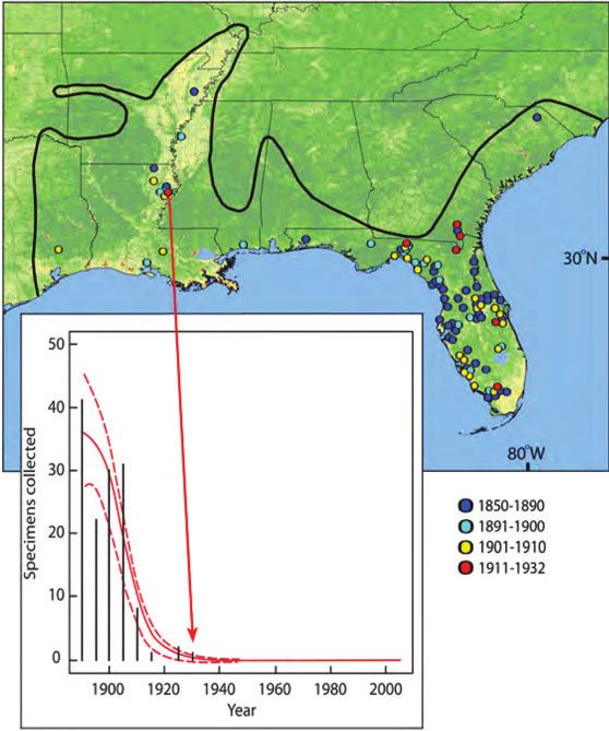
Figure 1. Spatial and temporal
distribution of Ivory-billed
Woodpecker specimens (black
line, approximate historical range
boundary of the Ivory-billed
Woodpecker [ Tanner 1942];
points, 1–6 museum specimens
with precise locality data [239
total specimens; Supporting
Information]; dark blue points,
collections made 1850–1890,
when specimen numbers in
museum collections were
increasing [Supporting
Information]; yellow, light blue,
and red points, collections made
1891–1932, when specimen
numbers were declining [see
inset]; solid red curve, data in
4-year interval bins fitted with
Poisson generalized additive
model; dashed red lines, 95% CI;
red arrow, originates in
northeastern Louisiana, where
the last specimen was collected in
1932).
through a network of professional collectors in the south- which the last museum specimen was collected legally
ern states, particularly Florida. As the species became pro- in 1932 (Jackson 2004).
gressively rarer during the 1870s and 1880s (Hasbrouck In short, the evidence indicates that the decrease in
1891), the demand for specimens increased, resulting in the number of Ivory-billed Woodpecker specimens col-
high retail prices and intensive unregulated hunting by lected between 1894 and 1932 reflects a true decline
professional collectors (Hasbrouck 1891; Snyder 2007; in abundance, rather than a decline in collection efforts,
Snyder et al. 2009). The number of specimens collected which were driven by free-market supply and demand, as
peaked between 1885 and 1894 and then declined rapidly evidenced by the high maximum prices for Ivory-billed
as local populations were extirpated by changes in land Woodpeckers at a time when the supply of specimens
use, subsistence and trophy hunting, and collecting for dried up (Snyder 2007; Snyder et al. 2009). The long his-
museums (Fig. 1 & Supporting Information). The de- tory of habitat loss from logging, and of sport and subsis-
cline in abundance and specimen accumulation rates oc- tence hunting, strongly suggests that the modest number
curred well before commercial hunting activities were of scientific specimens collected, in itself, contributed
effectively regulated by wildlife protection laws. Scien- relatively little to the woodpecker’s range-wide decline.
tific collecting permits for Ivory-billed Woodpeckers con- The diminishing curve of museum specimens collected
tinued to be issued until the early 1930s. After 1932, can be considered a proxy of total population size (Sup-
collecting was prohibited as concern for the species’ sur- porting Information).
vival increased. However, individuals continued to be To model the scientific specimen record as a proxy
sighted periodically for another decade. The last undis- of population size, we treated the years between 1893
puted sightings of the species occurred in 1944, in the (the starting year of the peak 4-year interval for specimen
same remnant population in northeastern Louisiana from collection) and 2008 (the final year of the most recent
Conservation Biology
Volume 26, No. 1, 2012Gotelli et al. 51
complete 4-year interval) as a series of 29 consecutive 4- was 0.0532. Suppose that, in 1929–1932, the total pop-
year intervals (Supporting Information). We fitted a Pois- ulation size (N) was 100, so that p ≈ 1/100 = 0.01. The
son generalized additive model to this series (Wood 2006; expected population size in 1941–1944 would then be
Supporting Information), estimated the expected num- nt = 0.0532/p = 5.32 birds. From the Poisson distribution
ber of records (µt ) in each 4-year interval after 1932, and with a mean of 5.32, the probability of persistence would
calculated a corresponding 95% CI (Fig. 1 & Supporting exceed 0.995. Therefore, if the 1929–1932 population
Information). was at least as large as 100 individuals, the species was
The last museum specimen was collected in 1932. If almost certainly present in 1941–1944. If the hypothet-
the total population size of the Ivory-billed Woodpecker ical 1929–1932 total population size was only 20, then
between 1929 and 1932 was N, then the proportion of p = 0.05. In this case, nt in 1941–1944 would be only
the population represented by this single specimen is 1.064, and the Poisson probability of presence would
p ≈ 1/N. One can interpret p as the per capita probabil- decrease to 0.655, which is still greater than the proba-
ity that a woodpecker would be collected as a specimen bility of absence (0.345). Thus, the generalized additive
(or unequivocally documented) within a single, 4-year model that we based on specimen data alone correctly im-
time interval. If one assumes this per-individual, condi- plied the persistence of the Ivory-billed Woodpecker in
tional probability of detection is roughly constant after the 1941–1944 interval, during which individuals were
the 1929–1932 interval, the expected number of speci- repeatedly sighted in a single dwindling population in
mens µt depends on the probability of detection p and Louisiana. However, in the following period, 1945–1948,
the population size nt in the tth 4-year interval: the expected number of records became 0.524, and in
this period the Poisson probability of absence (0.592)
μt = pnt .
exceeded the probability of presence (0.408).
From this relation, nt can be estimated for any subse-
quent time interval from the fitted µ̂ as
Analyses of Contemporary Census Data
nt ≈ μ̂t / p ≈ μ̂t N .
We analyzed contemporary avian census data collected
We treated the population size of Ivory-billed Wood- in the southeastern United States during the search for
peckers in any specific 4-year interval as a Poisson the Ivory-billed Woodpecker to estimate the probability
random variable. Thus, we estimated the probabil- of observing a species previously undetected by the cen-
ity of population persistence in the tth interval as sus. A 4-person team surveyed winter bird populations
1 − exp(−nt ), the total probability of the nonzero classes (December–February) at 4 sites deemed to be among the
of the Poisson distribution with mean nt (Supporting In- most promising for relictual populations of the Ivory-
formation). We assumed a Poisson distribution for 2 rea- billed Woodpecker (Rohrbaugh et al. 2007). Censuses
sons. First, because the sample size was relatively small, it were conducted from sunrise to sunset on foot and from
was statistically preferable for us to use a single-parameter canoes, and similar field methods were used at all census
model that could be estimated directly from the data (Mc- sites. (Raw census data [MST06–07] are available from
Cullagh & Nelder 1989). A 2-parameter negative binomial eBird [2009].)
distribution is a generalized form of the Poisson, but it Although no Ivory-billed Woodpeckers were found,
did not provide stable parameter estimates for these data. searchers generated standardized census data for other
Second, mechanistic population-growth models of birth species observed in potential Ivory-billed Woodpecker
and death processes can lead to a Poisson distribution of habitat (Rohrbaugh et al. 2007). We based our analyses
population sizes (Iofescu & Táutu 1973). on data from the 2006 to 2007 avian censuses from the
The assumption that the probability of detection per Congaree River, South Carolina (15,500 individuals, 56
individual (p) (but not the population’s size [nt ]) was species), Choctawhatchee River, Florida (6,282 individ-
constant over all the time intervals was conservative for uals, 55 species), Pearl River, Louisiana and Mississippi
the purpose of estimating the probability of population (3,343 individuals, 54 species), and Pascagoula River, Mis-
persistence. If this assumption were in error, and p ac- sissippi (6,701 individuals, 54 species; Supporting Infor-
tually increased after 1932 because increased detection mation).
effort was focused on a declining population, then our We evaluated whether the census efforts at these lo-
estimates represent a conservative upper bound for the calities were sufficient to discover an Ivory-billed Wood-
probability of population persistence. pecker if it had been present and derived a practical
Because the last undisputed sighting was in 1944, we stopping rule for deciding when to abandon the search
were able to conduct an important benchmark test of our in a particular site. An efficient stopping rule that in-
specimen-based model by estimating persistence proba- corporates rewards of discovery and costs of additional
bility in the 1941–1944 interval. With the specimen-based sampling should be triggered at the smallest sample size
generalized additive model, the expected number of q satisfying f 1 /q < c/R, where f 1 is the number of sin-
records for this interval (Fig. 1 & Supporting Information) gletons (species observed exactly once during a census),
Conservation Biology
Volume 26, No. 1, 201252 Specimen-Based Extinction Assessment
c is the cost of making a single observation, and R is the Table 1. Hypothetical total population sizes of Ivory-billed
reward for detecting each previously undetected species Woodpeckers from 1929 to 1932, the corresponding predicted
probability of persistence in the time interval 2005 to 2008, and the
(Rasmussen & Starr 1979). Because R for an Ivory-billed estimated extinction interval (the earliest period for which the
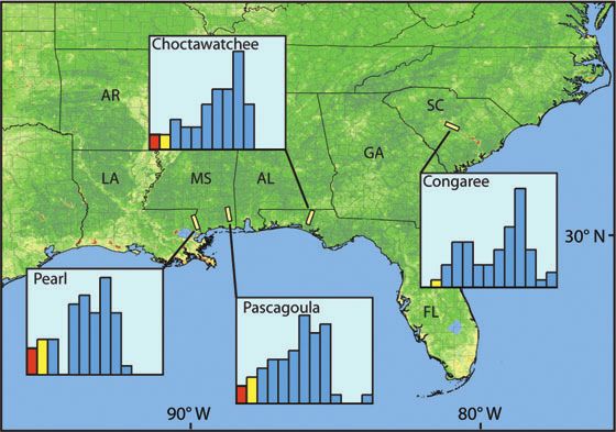
Woodpecker is extremely large relative to c, c/R is close probability of persistence isGotelli et al. 53 Figure 2. Avian data from 4 bottomland sites in the southeastern United States, where searches for Ivory-billed Woodpeckers were conducted in 2006 and 2007: Congaree River, South Carolina (15,500 individuals, 56 species), Choctawhatchee River, Florida (6,282 individuals, 55 species), Pearl River, Louisiana and Mississippi (3,343 individuals, 54 species), Pascagoula River, Mississippi (6,701 individuals, 54 species). Histograms depict the number of species represented by a particular number of individuals on an octave scale (1, 2, 3–4, 5–8, 9–16, . . . , 2049–4096), which is commonly used to represent species abundance data ( Magurran 2004) (red, singletons [species for which exactly 1 individual has been recorded in a census]; yellow, doubletons [species for which exactly 2 individuals have been recorded in a census]; y-axis range, 0–15 species). No singletons were detected at Congaree River. Pascagoula River site, the required additional number of Discussion observations was estimated at 4179, approximately two- thirds of the number sampled to date. Our results suggest that the probability of persistence At all 4 sites, the probability p∗ that the next individual in 2011 of the Ivory-billed Woodpecker was
54                                                                                            Specimen-Based Extinction Assessment

assume a constant search effort, are on the optimistic          conclusion that the Ivory-billed Woodpecker is now
side because the collective search effort for the Ivory-        extinct.
billed Woodpecker has increased tremendously since                 The reported rediscovery of the Ivory-billed Wood-
1932.                                                           pecker has been one of the most controversial findings in
   The exhaustive avian censuses carried out to date in         conservation biology, and the survey program designed
the search for the Ivory-billed Woodpecker (Fig. 2 & Sup-       to confirm that report among the most intensive and
porting Information) also make it unlikely that additional      costly. Certainly, such rigorous, quantitative rediscovery
species will be detected at these 4 sites (Table 2) with-       programs will not be implemented for most possibly ex-
out expending almost as much additional effort as has           tinct species; thus, the methods we used to analyze cen-
already been invested. Of course, even if extensive fur-        sus data for the woodpecker cannot be applied often.
ther censuses were to yield additional species, there is        Similarly, for many species, museum specimen series are
no guarantee that the Ivory-billed Woodpecker would be          either too meagre or too idiosyncratically obtained (Pyke
among them. At the Pearl River site, for example, more          & Ehrlich 2010) to justify the application of our Poisson
plausible candidates for new species observations are           generalized additive model.
American Woodcock (Scolopax minor) and Red-headed                  Nevertheless, when the data justify it, the analytical
Woodpecker (Melanerpes erythrocephalus).                        methods we developed can be applied to other retrospec-
   Inevitably, considerable uncertainty must be associ-         tive analyses of museum-collection records and to records
ated with the statistical estimation of extinction times        from standardized field surveys, 2 important sources of
from historical specimen records. For example, use of           data that are based on evidentiary standards (McKelvey
the Poisson generalized additive model to project spec-         et al. 2008). Moreover, our method can be adapted for
imen numbers (Fig. 1) cannot be rigorously justified for        use with Rout et al.’s (2009a, 2009b) analyses of eradica-
application to sparse data, and parameter estimates, such       tion programs for invasive species. These tools can help
as the size of the Ivory-billed Woodpecker population in        guide expectations of search-efforts and optimize the al-
1929–1932 (Table 1), can be difficult to establish.             location of limited conservation resources in the search
   In view of these uncertainties, an effective strategy is     for other rare species (Chadès et al. 2008) or for invasive
to analyze extinction times from a completely different         species that have putatively been eradicated (Rout et al.
statistical perspective and determine whether the results       2009a, 2009b).
are consistent. Elphick et al. (2010) and Roberts et al.
(2010) applied Solow’s (1993a, 2005) method, which is           Acknowledgments
derived from extreme value theory, to estimate the ex-
tinction year of the Ivory-billed Woodpecker. They based        We thank S. Haber and P. Sweet for providing informa-
their analyses on physical evidence of museum speci-            tion on Ivory-billed Woodpecker specimens in the Amer-
mens, photographs, and sound recordings as well as on           ican Museum of Natural History, C. Elphick for extensive
reports of visual sightings confirmed by independent ex-        comments on the manuscript, and M. Rivadeneira and
perts. These data were represented as a binary sequence         K. Roy for help in understanding their related work.
of annual presences (at least one individual detected in        N.J.G. and R.K.C. were supported by the U.S. National Sci-
year t) and absences (no individual detected in year t). El-    ence Foundation. A.C. and W.H. were funded by the Tai-
phick et al. (2010) and Roberts et al. (2010, their Table 2)    wan National Science Council. G.R.G. was supported by
based their analysis on 39 presences between 1897 and           the Alexander Wetmore Fund, Smithsonian Institution,
1944, which correspond to the quantitative data used            and the Center for Macroecology, Evolution, and Climate,
in our analyses (Supplemental Information) reduced to           University of Copenhagen. This study is a contribution of
simple yearly presence data plus additional records after       the Synthetic Macroecological Models of Species Diver-
1932.                                                           sity Working Group supported by the National Center for
   In spite of the differing assumptions and treatment of       Ecological Analysis and Synthesis, a Center funded by the
the data (discussed fully in Supporting Information), the       National Science Foundation, the University of California,
conclusions of Elphick et al. (2010) and Roberts et al.         Santa Barbara, and the State of California.
(2010) are qualitatively consistent with our findings.
Their analysis of physical evidence yielded a probable
extinction date for the Ivory-billed Woodpecker of 1941,        Supporting Information
with an upper 95% confidence interval of 1945 (Table 1 in
Elphick et al. 2010; Fig. 1 in Roberts et al. 2010). Although   The following information is available online: general
their estimated extinction dates differ from ours (1941         statistical methods for analysis of museum specimen
vs. 1980), our analyses of museum specimens (Fig. 1)            data (Appendix S1); compilation of Ivory-billed Wood-
and records from contemporary avian censuses (Fig. 2)           pecker museum specimen data (Appendix S2); statistical
and the alternative analyses of Roberts et al. (2010)           analyses of Ivory-billed Woodpecker museum specimen
and Elphick et al. (2010) all point to the inescapable          data (Appendix S3); statistical analyses of Ivory-billed

Conservation Biology
Volume 26, No. 1, 2012
Gotelli et al.                                                                                                                                         55

Woodpecker contemporary census data (Appendix S4);                             Elphick, C. S., D. L Roberts, and J. M. Reed. 2010. Estimated dates of re-
comparisons with other published analyses of Ivory-billed                          cent extinctions for North American and Hawaiian birds. Biological
                                                                                   Conservation 143:617–624.
Woodpecker extinctions (Appendix S5); frequency dis-
                                                                               Fitzpatrick, J. W., et al. 2005. Ivory-billed Woodpecker (Campephilus
tribution of museum specimen data (Appendix S6); fre-                              principalis) persists in continental North America. Science
quency counts of museum specimen data (Appendix                                    308:1460–1462.
S7); frequency distribution of binned specimen data (Ap-                       Good, I. J. 1953. The population frequencies of species and the estima-
pendix S8); fitted Poisson general additive model (Ap-                             tion of population parameters. Biometrika 40:237–264.
                                                                               Good, I. J. 2000. Turing’s anticipation of empirical Bayes in connection
pendix S9); persistence probabilities as a function of
                                                                                   with the cryptanalysis of the naval Enigma. Journal of Statistical
population size (Appendix S10); frequency counts for                               Computation and Simulation 66:101–111.
contemporary avian census data (Appendix S11); and                             Hahn, P. 1963. Where is that vanished bird? An index to the known
species counts at each of 4 census sites (Appendix S12).                           specimens of the extinct and near extinct North American species.
The authors are responsible for the content and func-                              Royal Ontario Museum, University of Toronto, Toronto.
                                                                               Hamer, A. J., S. J. Lane, and M. J. Mahony. 2010. Using probabilistic mod-
tionality of these materials. Queries (other than absence
                                                                                   els to investigate the disappearance of a widespread frog-species
of the material) should be directed to the corresponding                           complex in high-altitude regions of south-eastern Australia. Animal
author.                                                                            Conservation 13:275–285.
                                                                               Hasbrouck, E. M. 1891. The present status of the Ivory-billed Wood-
                                                                                   pecker (Campephilus principalis). Auk 8:174–186.
                                                                               Iofescu, M., and P. Táutu. 1973. Stochastic processes and applications
Literature Cited                                                                   in biology and medicine. Volume II. Models. Springer-Verlag, Berlin.
                                                                               Jackson, J. A. 2004. In search of the Ivory-billed Woodpecker. Smithso-
Audubon, J. J. 1832. Ornithological biography. E. L. Carey and A. Hart,            nian Institution Press, Washington, D.C.
   editors. Philadelphia, Pennsylvania.                                        Magurran, A. E. 2004. Measuring biological diversity. Blackwell Science,
Burgman, M. A., R. C. Grimson, and S. Ferson. 1995. Inferring threat               Oxford, United Kingdom.
   from scientific collections. Conservation Biology 9:923–928.                McCarthy, M. A. 1998. Identifying declining and threatened species
Burgman, M., B. Maslin, D. Andrewartha, M. Keatley, C. Boek, and M.                with museum data. Biological Conservation 83:9–17.
   McCarthy. 2000. Inferring threat from scientific collections: power         McCullagh, P., and J. A. Nelder. 1989. Generalized linear models. 2nd
   tests and an application to Western Australian Acacia species. Pages            edition. Chapman and Hall/CRC, Boca Raton, Florida.
   7–26 in S. Ferson and M. Burgman, editors. Quantitative methods             McKelvey, K. S., K. B. Aubry, and M. K. Schwartz. 2008. Using anecdotal
   for conservation biology. Springer-Verlag, New York.                            occurrence data for rare or elusive species: the illusion of reality and
Chadès, I., E. McDonald-Madden, M. A. McCarthy, B. Wintle, M. Linkie,             a call for evidentiary standards. BioScience 58:549–555.
   and H. P. Possingham. 2008. When to stop managing or sur-                   Pyke, G. H., and P. R. Ehrlich. 2010. Biological collections and ecologi-
   veying cryptic threatened species. Proceedings of the National                  cal/environmental research: a review, some observations and a look
   Academy of Sciences of the United States of America 105:13936–                  to the future. Biological Reviews 85:247–266.
   13940.                                                                      Rasmussen, S., and N. Starr. 1979. Optimal and adaptive search for a
Chao, A. 2005. Species estimation and applications. Pages 7907–7916 in             new species. Journal of American Statistical Association 74:661–
   N. Balakrishnan, C. B. Read, and B. Vidakovic, editors. Encyclopedia            667.
   of statistical sciences 12. 2nd edition. Wiley, New York.                   Regan, T. J., M. A. McCarthy, P. W. J. Baxter, F. Dane Panetta, and H. P.
Chao, A., R. K. Colwell, C.-W. Lin, and N. J. Gotelli. 2009. Sufficient sam-       Possingham. 2006. Optimal eradication: when to stop looking for
   pling for asymptotic minimum species richness estimators. Ecology               an invasive plant. Ecology Letters 9:759–766.
   90:1125–1133.                                                               Rivadeneira, M. M., G. Hunt, and K. Roy. 2009. The use of sighting
Collen, B., A. Purvis, and G. M. Mace. 2010. When is a species really              records to infer species extinctions: an evaluation of different meth-
   extinct? Testing extinction inference from a sighting record to in-             ods. Ecology 90:1291–1300.
   form conservation assessment. Diversity and Distributions 16:755–           Roberts, D. L. 2006. Extinct or possibly extinct? Science 312:997.
   764.                                                                        Roberts, D. L., C. S. Elphick, and J. M. Reed. 2010. Identifying anomalous
Collinson, J. M. 2007. Video analysis of the escape flight of Pileated             reports of putatively extinct species and why it matters. Biological
   Woodpecker Dryocopus pileatus: does the Ivory-billed Wood-                      Conservation 24:189–196.
   pecker Campephilus principalis persist in continental North Amer-           Roberts, D. L., and A. R. Solow. 2003. When did the dodo become
   ica? BMC Biology 5:8.                                                           extinct? Nature 426:245.
Colwell, R. K., and J. A. Coddington. 1994. Estimating terrestrial bio-        Rohrbaugh, R., M. Lammertink, K. Rosenberg, M. Piorkowski, S. Barker,
   diversity through extrapolation. Philosophical Transactions of the              and K. Levenstein. 2007. 2006–07 Ivory-billed Woodpecker sur-
   Royal Society of London Series B: Biological Sciences 345:101–                  veys and equipment loan program. Report. Cornell Laboratory of
   118.                                                                            Ornithology, Ithaca, New York. Available from http://www.birds.
Diamond, J. M. 1987. Extant unless proven extinct? Or, extinct unless              cornell.edu/ivory/pdf/FinalReportIBWO_071121_TEXT.pdf (acces-
   proven extant? Conservation Biology 1:77–79.                                    sed December 2010).
Eames, J. C., H. Hla, P. Leimgruber, D. S. Kelly, S. M. Aung, S. Moses, and    Rout, T. M., Y. Salomon, and M. A. McCarthy. 2009a. Using sighting
   S. N. Tin. 2005. Priority contribution. The rediscovery of Gurney’s             records to declare eradication of an invasive species. Journal of
   Pitta Pitta gurneyi in Myanmar and an estimate of its population size           Applied Ecology 46:110–117.
   based on remaining forest cover. Bird Conservation International            Rout, T. M., C. J. Thompson, and M. A. McCarthy. 2009b. Robust deci-
   15:3–26.                                                                        sions for declaring eradication of invasive species. Journal of Applied
eBird. 2009. An online database of bird distribution and abundance.                Ecology 46:782–786.
   Avian Knowledge Network and Cornell Laboratory of Ornithology,              Sibley, D. A., L. R. Bevier, M. A Patten, and C. S. Elphick. 2006. Comment
   Ithaca, New York, and National Audubon Society, Washington, D.C.                on ‘Ivory-billed Woodpecker (Campephilus principalis) persists in
   Available from http://www.avianknowledge.net (accessed Decem-                   continental North America. Science Online 311:DOI: 10.1126/sci-
   ber 2010).                                                                      ence.1114103.

                                                                                                                                    Conservation Biology
                                                                                                                                    Volume 26, No. 1, 2012
56 Specimen-Based Extinction Assessment Snyder, N. F. R. 2007. An alternative hypothesis for the cause of Solow, A. R., and D. L. Roberts. 2003. A nonparametric test the Ivory-billed Woodpecker’s decline. Monograph of the Western for extinction based on a sighting record. Ecology 84:1329– Foundation of Vertebrate Zoology 2:1–58. 1332. Snyder, N. F. R., D. E. Brown, and K. B. Clark. 2009. The travails of two Tanner, J. T. 1942. The Ivory-billed woodpecker. Research report 1. woodpeckers: Ivory-bills and Imperials. University of New Mexico National Audubon Society, New York. Press, Albuquerque. U.S. Fish and Wildlife Service. 2009. Recovery plan for the Ivory-billed Sodhi, N. S., et al. 2008. Correlates of extinction proneness in tropical Woodpecker (Campephilus principalis). U.S. Fish and Wildlife Ser- angiosperms. Diversity and Distributions 14:1–10. vice, Atlanta. Solow, A. R. 1993a. Inferring extinction from sighting data. Ecology Vogel, R. M., J. R. M. Hosking, C. S. Elphick, D. L. Roberts, and J. M. 74:962–964. Reed. 2009. Goodness of fit of probability distributions for sightings Solow, A. R. 1993b. Inferring extinction in a declining population. as species approach extinction. Bulletin of Mathematical Biology Journal of Mathematical Biology 32:79–82. 71:701–719. Solow, A. R. 2005. Inferring extinction from a sighting record. Mathe- Wood, S. N. 2006. Generalized additive models: an introduction with matical Biosciences 195:47–55. R. Chapman and Hall/CRC Press, Boca Raton, Florida. Conservation Biology Volume 26, No. 1, 2012
Appendix S1. A general statistical method for estimating the probability of persistence from

museum specimen records

Step 1. The analysis uses museum specimen frequency data in the form of yearly records as in

Appendix S6. Because the raw (yearly) counts typically vary greatly from one year to the next, it

is difficult to model the temporal trend as a smooth curve. Therefore, it will usually be necessary

to first group (bin) the data into multi-year intervals to reveal prominent temporal trends. The

results of the statistical anlaysis are potentially sensitive to the size of the binned interval.

Typically, large intervals (i.e. more data points per bin) lead to a smaller variance but a larger

bias, whereas narrow intervals (fewer data points per bin) lead to a smaller bias but a larger

variance. Appendix S3 demonstrates how to determine an optimal bin size using the Ivory-billed

Woodpecker data as an example.

Step 2. After binning, there are T time-interval bins. Let Yt , t = 1, 2, .., T be the the number of

records for the t-th period, where t =1 is the first binned interval. We first fit a smoothed curve to

the specimen data. If we can assume that the fitted curve of specimen numbers generally reflects

population size pattern, then the fitted series can be used to estimate population abundance.

There are many statistical models can be used to model a time series (and any covariate predictor

variables). We use a generalized additive model (GAM), which combines the properties of

generalized linear models with additive models. The GAM model specifies a distribution

function for Yt (Poisson, normal, binomial etc.) and a link function g, which relates μt = E(Yt) to

the time-varying covariates {x1t , x2t ,..., xmt ; t 1, 2,..., T } as:

                           g( t )         f1 ( x1t )   f 2 ( x2 t ) ....   f m ( xmt ) .        (S1)

Here “additive” refers to the sum of the functions of f1, f2,…, fm. Each function of f1, f2,…, fm

can be parametric (including linear or quadratic or generalized linear models) or non-parametric

                                                             1
(including nonparametric regression). Thus the GAM is flexible and can be fit to many different
kinds of temporal trends. To estimate each f(t), we fit the widely used penalized regression spline
model (Wahba 1990, Ruppert et al. 2006) and selected cubic regression splines as the basis for
constructing each f(t). The penalized regression spline model controls the degree of smoothness
by adding a penalty to the likelihood function. This model usually provides a better fit than
parametric linear or quadratic models. The implementation of the penalized regression spline can
be found in many software applications, including the Proc Glimmix in SAS. A widely used and
free software is the mgcv package in R (Wood, 2006) which can be downloaded from
http://www.r-project.org/. We used Ivory-billed Woodpecker data as an example in Appendix S3
to illustrate the model fitting procedures.
Step 3. After the model fitting, we obtain a fitted time series { ˆt ; t 1, 2,..., T } . Let k be the latest
time period with non-zero specimen records. That is, after time period k, there are no specimen
records (Yt = 0 for t > k). For a hypothetical population size N in the time interval k, define p as
the probability that any individual would be collected as a specimen within a single time interval.
This probability p in the k-th period can be estimated by the sample proportion Yk/N. We assume
this probability p is a constant in all intervals after time k. Next we estimate the expected
population size in any time interval t > k as nt ˆt / p ˆ t N / Yk . The probability of persistence
(of at least one individual) in the t-th interval can be estimated as P(nt 0) .
The fitting results in Step 3 can be used to determine an optimal bin size for a particular data set.
For each size interval that is tested, we obtain the fitted series and calculate the adjusted R-
square as a measure of the closeness of the fitted values and the data. The bin size that yields the
largest adjusted R2 from the fitted models is then selected (e.g., a 4-year interval for the Ivory-
2billed Woodpecker data).
Supplementary Literature Cited
Ruppert, D., Wand, M. P., and R. J. Carroll. 2006. Semiparametric regression. Cambridge
University Press, New York.
Wahba, G. 1990. Smoothing models for observational data. SIAM, Philadelphia.
Wood, S. N. 2006. Generalized additive models: An introduction with R. Chapman and
Hall/CRC Press, Boca Raton.
3Appendix S2. Compilation of museum specimen data for the Ivory-billed Woodpecker and
historical trends in collecting activity.
Specimen data were compiled from Hahn (1963) with additional data from Jackson (2004) and
Ornis (2004). More than 400 Ivory-billed Woodpecker specimens are deposited in North
American and European museums. Many specimens prepared as taxidermy mounts during the
first half of the 19th century lack museum labels with date and locality data. However, the quality
of data accompanying specimens collected after 1880 was relatively good because the species
was already considered rare by ornithologists and specimens were highly coveted by museums
and private collectors, both of which placed a premium on well-prepared skins and accurate
locality data.
A substantial proportion of specimens obtained by professional collectors after 1890 were sold
directly to museums and private collectors (Jackson 2004; Snyder et al. 2009). Professional
collectors often employed networks of local hunters to obtain specimens. In the early 1890s,
Arthur T. Wayne, one of the more prolific collectors of Ivory-billed Woodpeckers in Florida, paid
local hunters and trappers up to US$5 ($123 in today’s currency) for specimens in good
condition (Snyder et al. 2009). For comparison, unskilled laborers in rural regions of the
southeastern United States were paid < $1 per day during the 1890s (U.S. Bureau of Labor 1904).
Cash bounties offered by professional collectors and specimen dealers were potent incentives for
local woodsmen to seek out relictual populations. During 1894, specimens were offered for retail
sale at $15 per specimen ($369 in today’s currency; Jackson 2004). Retail valuations of
specimens more than tripled after 1900 as demand greatly outstripped supply (Jackson 2004).
None of the states (Texas, Louisiana, Mississippi, Georgia, Florida, South Carolina) known to
1support Ivory-billed Woodpecker populations after 1900 (Tanner 1942; Jackson 2004) had laws
protecting the species from commercial collecting in 1903 (Ducher 1903).
Despite the enormous economic incentive, specimen production decreased markedly after 1906
as most of the well-known populations were extirpated. Legal prohibition of commercial
collecting did not occur until the passage of the Migratory Bird Treaty Act of 1918, but effective
regulation of hunting activity of any kind was rare or nonexistent in remote regions of the rural
southeastern United States through the 1930s. State-sanctioned collecting permits for Ivory-
billed Woodpeckers were issued as late as 1932 (Jackson 2004). Populations were also subjected
to intense subsistence hunting and curiosity shooting (Snyder et al. 2009). These sources of
mortality are thought to have greatly outweighed the impact of specimen collecting on relict
populations in the 20th century (Snyder et al. 2009).
It is likely that the decline of Ivory-billed Woodpecker populations began more than a
millennium ago when American Indian populations expanded greatly in eastern North America
after the introduction of maize cultivation from Mexico. Prized for their bills and plumage, this
species figures frequently in Mississippian culture (800-1500 CE) burial goods, including carved
pipe bowls, shell gorgets, and ceramics (Brain & Phillips 1996; Jackson 2004). Ivory-billed
Woodpecker plumage and bills were traded as curios and ceremonial objects by American
Indians as late as the 19th century, whereas intensive subsistence hunting, trophy hunting, and
scientific collecting by European Americans continued through the early 20th century (Jackson
2004; Snyder et al. 2009).
2Range contraction undoubtedly began in earnest with clearing of forests along the lower Atlantic
coastal plain in the Colonial period. The final period of extinction started after the Civil War,
when northern timber companies purchased huge tracts of cheap "government-owned" land in
the southern states. Most virgin timber was cut between 1870 and 1930 (Williams 1989).
Remnant stands lasted until the early 1940s, but the demand for lumber during WW II for gun
stocks, cargo pallets, and plywood for PT boats finished those tracts off (and the woodpeckers
they harbored), including the Singer Tract and another large parcel near Rosedale, Mississippi
(Jackson 2004; Snyder et al. 2009).
In short, the museum specimens on which our analysis is based represent the tail of a long
decline in populations. Our models are based on the premise that the dwindling rate of specimen
accumulation in museum collections mirrors steep population declines throughout the historic
range of the species, particularly given the premium prices paid for specimens by museums and
private collectors after 1880.
Analyses were limited to dated specimens with locality data (at least state). Date refers to the
date of collection rather than the accession date in museums. A few specimens of doubtful
provenance or lacking verifiable dates on museum labels were omitted from the analysis.
Although we only used specimens with reliable locality data, it should be noted that our analyses
are not spatially structured, and instead model the temporal decline of the Ivory-billed
Woodpecker after 1880 throughout its geographic range.
3Supplementary Literature Cited
Brain, J. P., and P. Phillips. 1996. Shell gorgets. Styles of the late prehistoric and protohistoric
Southeast. Peabody Museum Press, Peabody Museum of Archaeology and Ethnology,
Harvard University, Cambridge.
Dutcher, W. 1903. Report of the A. O. U. committee on the protection of North American birds.
Auk 20:101-159.
Hahn, P. 1963. Where is that vanished bird? An index to the known specimens of the extinct and
near extinct North American species. Royal Ontario Museum, University of Toronto.
Jackson, J. A. 2004. In search of the Ivory-billed Woodpecker. Smithsonian Press, Washington,
D.C.
Ornis. 2004. Ornithological Information System. http://ornisnet.org. Accessed 20 December
2010.
Snyder, N. F. R., D. E. Brown, and K. B. Clark. 2009. The travails of two woodpeckers: Ivory-
bills and Imperials. University of New Mexico Press, Albuquerque.
United States Bureau of Labor. 1904 Wages and hours of labor. Nineteenth Annual Report of the
Commissioner of Labor. Department of Commerce and Labor. Government Printing
Office, Washington, D.C., 976 p.
Williams, M. 1989. Americans and their forests: A historical geography. Cambridge University
Press, Cambridge.
4Appendix S3. Application to Ivory-billed Woodpecker museum specimen frequency data
In this Appendix, we apply the general estimation procedures in Appendix S1 to the Ivory-billed
Woodpecker specimen data and present details that are specific to this data set. Because the
yearly specimen totals for Ivory-billed Woodpecker in museums (Appendix S7; panel A of
Appendix S6) varied considerably, we binned these data in 4-year intervals to smooth the series
(Appendix S8; panel B of Appendix S6). The interval size of 4-year was selected because it
generated the largest adjusted R2 compared with other bin intervals from 1-year to 5-years
(adjusted R2 values were 50%, 69%, 82%,86%, and 84% respectively). The time series for
collected specimens in the binned intervals (vertical black lines in Fig. 1) includes not only the
counts of specimens collected from 1893 to 1932, but also the uninterrupted string of zeroes
from 1933 to 2008, during which no additional specimens were collected. To our knowledge,
scientific collecting permits for Ivory-billed Woodpeckers were not issued after 1932 and no
additional specimens were collected after this date. For this reason, projection of the curve in Fig.
1, detailed below, must be interpreted as the expected number of IBW specimens that could have
been collected, had hunting continued, in each four-year interval after 1932, on the assumption
that the decline illustrated in Appendix S6 continued on the same trajectory after 1932.
We fitted a smoothed curve to the museum specimen data (solid and dashed red lines in text Fig.
1) and used the fitted series to estimate Ivory-billed Woodpecker abundance in each 4-year
interval. We then converted the projected abundance into an estimate of the probability of
persistence of the woodpeckers in each 4-year interval, including the most recent complete
interval of 2005-2008.
1As discussed in the main text, we assume that the decrease in specimens after 1894 reflects a true
decline in Ivory-billed Woodpecker abundance. To model this decline, we assume that Y t is a
Poisson random variable with mean E (Yt ) = µt where Y t is the number of records for the t-th
four-year period, where t =1 stands for the time period 1893-1896 (the interval with the greatest
number of specimens). We fitted a Poisson GAM to the data after the specimen peak of 1893. In
the model, {Y t ; t = 1, 2, …} have different means due to decreasing population size, and the
means are dependent on time. We considered a log link function and the following simple form
of a GAM in Eq. (S1) with time as the sole predictor variable:
log µt= α + f (t ) , (S2)
where α denotes an unknown baseline constant and f(t) denotes an unknown smooth function of
time. Both α and f(t) are estimated from the data.
We used the mgcv package (Wood 2006) in the R software environment (R Development Core
Team 2008) to carry out the fitting and computation of the penalized regression spline model
(Wahba 1990; Ruppert et al. 2006), We used cubic regression splines (Wahba 1990; Ruppert et al.
2006) to construct a smooth function f(t). For these data, the goodness of fit test yielded a chi-
squared statistic χ2 = 21.95 with 25.7 effective degrees of freedom. From the chi-square
distribution, the P-value = 0.68, implying that the fit of the model to the data was adequate. The
fitted model projects the decline in specimen abundance after 1893 (Fig. 1, Appendix S9) into
more recent time intervals. We focus on inference after 1932 because the last specimen was
collected in that year.
To relate the estimated number of Ivory-billed Woodpecker records in each four-year interval to
2the corresponding estimated population size, we define p as the probability that any individual,
living woodpeckers would be collected as a specimen or otherwise reliably detected and
recorded within a single, 4-year time interval. Because the last specimen was collected during the
1929-32 interval, and collecting was illegal after 1932, this interval represents the latest
opportunity to infer p from specimen data. Assume the total living population size from 1929-32
is N, then p is approximately 1/N because there was only one specimen collected in this interval.
Thus, we have p ≈ 1 / N in the interval 1929-32. For purposes of the model, we assume that
probability of detection p is roughly a constant after 1932. In fact, the intensity of searches for
Ivory-billed Woodpecker increased substantially after the last known population in Louisiana
disappeared in 1944. If p increased with time, then our analyses over-estimate persistence
probabilities.
Given a hypothetical value of the 1929-32 population size N, we can then estimate the expected
population size of Ivory-billed Woodpeckers in time interval t after 1932 as nt ≈ µˆ t / p ≈ µˆ t N .
Assuming the population size in any time interval is a Poisson random variable, the probability
of persistence (of at least one individual) in the t-th interval can be estimated as 1 − exp(−nt ) ,
which is the probability that a Poisson random variable with mean n t takes a non-zero value
(Table S4).
Supplementary Literature Cited
R Development Core Team. 2008. R: A language and environment for statistical computing. R
Foundation for Statistical Computing, Vienna.
Ruppert, D., Wand, M. P., and R. J. Carroll. 2006. Semiparametric regression. Cambridge
University Press, New York.
3Wahba, G. 1990. Smoothing models for observational data. SIAM, Philadelphia.
Wood, S. N. 2006. Generalized additive models: An introduction with R. Chapman and
Hall/CRC Press, Boca Raton.
4Appendix S4. Statistical analysis of field survey data
Our statistical method for analyzing census data is based principally on the concept of the Good-
Turing frequency formulas (Good 1953, 2000), which helped the British decode German military
ciphers for the Wehrmacht Enigma cryptographic machine during World War II. Alan Turing is
considered to be the founder of modern computer science. His non-intuitive idea (an empirical
Bayesian approach), as applied to the Ivory-billed Woodpecker search problem, is that inference
regarding the probable number of undetected species depends on frequencies of rare species in
the same census area. To apply this concept to our multinomial model for the Ivory-billed
Woodpecker search problem, the species pool considered must be sufficiently large, frequency
data for rare (detected) species must be available, and the sample size should be large.
Ivory-billed Woodpeckers are (or were) conspicuous, diurnal, and sedentary, occupying year-
round territories (Tanner 1942; Jackson 2004). For the purpose of analysis, the pool of species
could be limited appropriately to species that are known to be sedentary, year-round residents of
bottomland forests at the four census sites. We expanded the analyses, however, to include both
resident and migratory species that normally winter in floodplain forest habitats, including early
successional regeneration in canopy gaps. Expanding the sampling pool in this way increases
information about rare species, and therefore potentially increases the estimated number of
undetected species that might be present. We included some species found along roadsides in
bottomland forested habitats (e.g., Mourning Dove) that typically occur in agricultural areas and
old-fields. However, species strongly associated with agriculture and pastures (e.g., Killdeer,
Eastern Meadowlark) were excluded from the analyses. Herons, cormorant, anhinga, ducks, and
coot were excluded, but we included a few species generally associated with rivers and oxbow
1You can also read