Repeat mapping of snow depth across an alpine catchment with RPAS photogrammetry - The Cryosphere
←
→
Page content transcription
If your browser does not render page correctly, please read the page content below
The Cryosphere, 12, 3477–3497, 2018
https://doi.org/10.5194/tc-12-3477-2018
© Author(s) 2018. This work is distributed under
the Creative Commons Attribution 4.0 License.

Repeat mapping of snow depth across an alpine catchment with
RPAS photogrammetry
Todd A. N. Redpath1,2 , Pascal Sirguey2 , and Nicolas J. Cullen1
1 Department    of Geography, University of Otago, Dunedin, 9016, New Zealand
2 National   School of Surveying, University of Otago, Dunedin, 9016, New Zealand

Correspondence: Todd A. N. Redpath (todd.redpath@otago.ac.nz)

Received: 14 May 2018 – Discussion started: 6 June 2018
Revised: 8 September 2018 – Accepted: 3 October 2018 – Published: 8 November 2018

Abstract. Being dynamic in time and space, seasonal snow          relevant to similar applications of surface and volume change
represents a difficult target for ongoing in situ measurement     analysis, this study demonstrates a repeatable means of accu-
and characterisation. Improved understanding and modelling        rately mapping snow depth for an entire, yet relatively small,
of the seasonal snowpack requires mapping snow depth at           hydrological catchment (∼ 0.4 km2 ) at very high resolution.
fine spatial resolution. The potential of remotely piloted air-   Resolving snowpack features associated with redistribution
craft system (RPAS) photogrammetry to resolve spatial vari-       and preferential accumulation and ablation, snow depth maps
ability of snow depth is evaluated within an alpine catch-        provide geostatistically robust insights into seasonal snow
ment of the Pisa Range, New Zealand. Digital surface mod-         processes, with unprecedented detail. Such data will enhance
els (DSMs) at 0.15 m spatial resolution in autumn (snow-free      understanding of physical processes controlling spatial dis-
reference) winter (2 August 2016) and spring (10 Septem-          tributions of seasonal snow and their relative importance on
ber 2016) allowed mapping of snow depth via DSM differ-           varying spatial and temporal scales.
encing. The consistency and accuracy of the RPAS-derived
surface was assessed by the propagation of check point resid-
uals from the aero-triangulation of constituent DSMs and
via comparison of snow-free regions of the spring and au-
tumn DSMs. The accuracy of RPAS-derived snow depth was            1   Introduction
validated with in situ snow probe measurements. Results
for snow-free areas between DSMs acquired in autumn and           Seasonal snow provides a globally important water resource
spring demonstrate repeatability yet also reveal that elevation   (Mankin et al., 2015; Sturm et al., 2017), which is highly
errors follow a distribution that substantially departs from a    variable in space and time (Clark et al., 2011). Difficulties
normal distribution, symptomatic of the influence of DSM          associated with collecting field observations limit the char-
co-registration and terrain characteristics on vertical uncer-    acterisation and understanding of spatial variability in snow
tainty. Error propagation saw snow depth mapped with an           depth and, in turn, our ability to improve spatially distributed
accuracy of ± 0.08 m (90 % c.l.). This is lower than the char-    modelling of seasonal snow. While insight can be gained via
acterization of uncertainties on snow-free areas (±0.14 m).       modelling on moderate to large scales (Winstral et al., 2013),
Comparisons between RPAS and in situ snow depth measure-          resolving the fine-scale variability and its controlling pro-
ments confirm this level of performance of RPAS photogram-        cesses remains limited by the ability to capture such variabil-
metry while also highlighting the influence of vegetation on      ity in the field (Clark et al., 2011). Since water storage within
snow depth uncertainty and bias. Semi-variogram analysis          a snowpack is a function of snow depth and density, and the
revealed that the RPAS outperformed systematic in situ mea-       former exhibits higher spatial variability than the latter, ad-
surements in resolving fine-scale spatial variability. Despite    vances in measuring snow depth at high spatial resolution of-
limitations accompanying RPAS photogrammetry, which are           fer promise for improved estimates of snow water equivalent
                                                                  (SWE) (Harder et al., 2016).

Published by Copernicus Publications on behalf of the European Geosciences Union.
3478                                     T. A. N. Redpath et al.: Repeat mapping of snow depth across an alpine catchment

   Historically, studies of seasonal snow processes have re-        and logistical challenges of placing equipment in situ in
lied on in situ observations. With biweekly temporal resolu-        complex terrain. Airborne lidar provides a balance of spa-
tion, Anderson et al. (2014) gained substantial insights into       tial resolution and accurate surface elevation measurement
physical controls on seasonal snow processes, albeit with a         and, combined with density estimates, can provide SWE es-
dependence on statistical scaling to relate transect-scale ob-      timates on the catchment scale across substantial areas of
servations to basin-scale processes. Alternatively, the nature      hundreds of square kilometres (Painter et al., 2016). High
of automated snow measurement instrumentation often pre-            financial costs and logistical challenges, however, preclude
cludes continuous in situ measurement across networks suf-          regular airborne lidar data capture in many regions globally.
ficiently dense to characterise fine-scale spatial variability.     Treichler and Kääb (2017) assessed ICESat lidar data, which
Kinar and Pomeroy (2015) provide a comprehensive review             is designed primarily for measuring surface elevation over
of instrumentation and techniques for measuring snow depth          polar regions to characterise seasonal snow depth in subpo-
and characterising snowpacks. In summary, while instrumen-          lar southern Norway. Despite reasonable estimates of snow
tation and methodologies exist for obtaining accurate and           depth, measurements were accompanied by relatively large
temporally continuous, measurements of snow depth and re-           errors for most temperate locations. ICESat measurements
lated snowpack properties at point locations, adequately re-        are also limited by their punctual nature and footprint, yield-
solving the high spatial variability of snow depth remains a        ing a relatively sparse and coarse spatial distribution, in turn
challenge. This is exacerbated by local field conditions, such      complicating inferences about spatial variability.
as exposure to wind or the complexity of the topography and            Recent technological advances, including the miniaturi-
vegetation further increasing the spatial variability in snow       sation of imaging and positioning sensors, as well as im-
depth (Clark et al., 2011; Kerr et al., 2013; Winstral and          provements in battery power and autonomous navigation
Marks, 2014).                                                       have significantly lowered the barriers associated with a re-
   Remote sensing has provided substantial advances in              motely piloted aircraft system (RPAS, also known as un-
quantification of seasonal snow variability, with imaging sen-      manned aerial systems, UAS, and unmanned aerial vehicles)
sors supporting spatial and temporal resolutions that allow a       operation (Watts et al., 2012). This, combined with ever-
range of scales to be explored. Space-borne satellite imagers       increasing computing power and significant improvements
provide a synoptic view and accompanying step-change ca-            in machine-vision for dense photogrammetric reconstruction
pability in capturing properties of snow-covered areas, al-         (Hirschmuller, 2008; Lindeberg, 2015), provides new op-
though trade-offs exist between competing spatial, spectral         portunities to map small areas photogrammetrically at very
and temporal resolutions (Dozier, 1989; Nolin and Dozier,           high resolution in a temporally flexible, on-demand, fashion.
1993; Hall et al., 2002, 2015; Sirguey et al., 2009; Malen-         Examples of RPAS use related to mapping snow depth are
ovský et al., 2012; Rittger et al., 2013; Roy et al., 2014;         promising but tend to apply to sub-catchment scales and to
Bessho et al., 2016). Passive and active microwave sensors          not fully characterise the uncertainty associated with pho-
offer the capacity to retrieve estimates of snow water equiva-      togrammetric modelling (Vander Jagt et al., 2015; Bühler
lent directly from space-borne platforms but also suffer sub-       et al., 2016; De Michele et al., 2016; Harder et al., 2016,
stantial limitations, including coarse spatial resolution in the    Cimoli et al., 2017; Avanzi et al., 2018). Furthermore, most
case of passive microwave sensors and complexities in suc-          RPAS studies of snow depth to date have mapped terrain
cessfully processing snow signals and accounting for com-           of relatively low complexity (e.g. Avanzi et al., 2018; Fer-
plex terrain in the case of both passive and active sensors         nandes et al., 2018). Additionally, with a few exceptions
(Lemmetyinen et al., 2018). Despite the progress in remotely        (e.g. Harder et al., 2016; Bühler et al., 2017; Marti et al.,
mapping snow, reliable determination of snow depth, partic-         2016), previous studies have often relied on multirotor plat-
ularly in complex terrain, remains challenging. Modern, very        forms despite their relatively short endurance and reduced
high-resolution stereo-capable imagers show promise for re-         spatial coverage relative to fixed-wing alternatives. Merit re-
trieving snow depth over large areas from space, although           mains in characterising fine-scale variability in snow depth
the influence of topography on uncertainties and complica-          distribution across an entire catchment, a scale that fixed-
tions introduced by shadows in alpine terrain demand atten-         wing RPAS can more easily capture. However, increased ter-
tion (Marti et al., 2016).                                          rain complexity and the magnitude of the image block can,
   Advances in light detection and ranging (lidar) technolo-        in turn, challenge photogrammetric modelling. Determina-
gies have become increasingly relevant for measurement of           tion of snow depth via RPAS photogrammetry relies first on
snow depth, firstly from air (Deems et al., 2013; Painter et al.,   the reconstruction of three-dimensional scenes from a set of
2016) and more recently from space-borne platforms (Tre-            overlapping images and then on the principal of differencing
ichler and Kääb, 2017). Of the three modes of lidar data            between temporally subsequent surfaces, provided by point
capture, terrestrial laser scanning (TLS) (e.g. Revuelto et al.,    clouds or digital surface models (DSMs) (Vander Jagt et al.,
2016) offers the best performance in terms of precision and         2015; Harder et al., 2016). A snow-free surface provides a
accuracy. TLS can resolve snow depth on a fine scale across         reference data set for absolute snow depth, while changes in
relatively large areas but remains limited by view-obstruction      snow distribution through winter can be assessed by com-

The Cryosphere, 12, 3477–3497, 2018                                                     www.the-cryosphere.net/12/3477/2018/
T. A. N. Redpath et al.: Repeat mapping of snow depth across an alpine catchment 3479
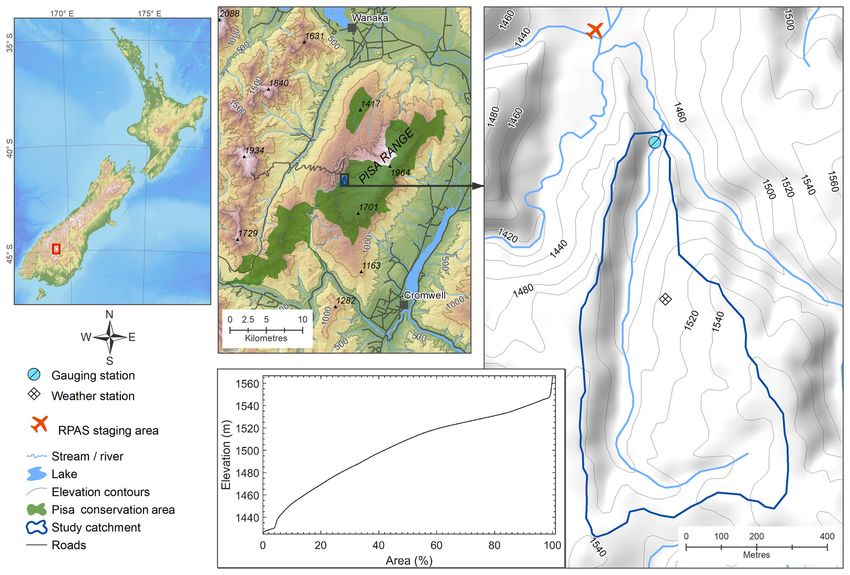
Figure 1. Location and hypsometry of the study catchment within the Pisa Range, New Zealand.
paring surfaces obtained while snow cover is present in the ploring and assessing the potential of RPAS photogramme-
catchment. Because changes in snow depth through time, ei- try for measuring seasonal snowpack, this study has broader
ther through processes of accumulation, ablation or redistri- implications for the wider field of modern close-range pho-
bution, may be subtle, the repeatability and vertical accuracy togrammetry, as typically implemented from low-cost (rel-
achieved by photogrammetric modelling is paramount. The ative to manned systems) unmanned systems. While con-
aim of this paper is to test a methodology for retrieving snow sidered here in terms of seasonal snow, the characterisation
depth across an entire catchment via RPAS photogrammetry of RPAS photogrammetry performance presented also ap-
from a fixed-wing platform. We seek to evaluate the perfor- plies to other applications involving three-dimensional sur-
mance, limitations and usefulness of this approach and assess face and/or volume change analysis.
how well snow depth can be resolved on the catchment scale.
Associated challenges include minimising spatial uncertain-
ties sufficiently to reliably detect changes in snow depth over 2 Study site
time, with a decimetre level of vertical accuracy targeted,
while also reducing the need and complication of extensive The study catchment (Fig. 1), a tributary of the Leopold
in situ collection of ground control points (GCPs). This ap- Burn located in the Pisa Range of the Southern Alps/Kā
proach was assessed during a campaign of winter RPAS- Tiritiri-o-te-Moana of New Zealand (44.882◦ S, 169.081◦ E),
based photogrammetric surveys of an alpine catchment in the is 0.41 km2 in size and has been the subject of prior snow-
Pisa Range, New Zealand, was undertaken. hydrology investigations (Sims and Orwin, 2011). Elevation
The paper describes the field site, field and photogram- of the catchment ranges between 1440 and 1580 m a.s.l. with
metric methods, as well as the quality and accuracy assess- a near-uniform area-elevation distribution (Fig. 1). The av-
ment. Results are considered in terms of the validation and erage slope is moderate, with 80 % of the catchment hav-
repeatability of the method, as well as considering the spa- ing a surface slope of 24◦ or less. The catchment runs north
tial distribution of snow within the catchment. The discus- to south and is drained by a small stream. While east of
sion addresses the performance of RPAS photogrammetry in the Main Divide of the Southern Alps, the Pisa Range is
this context, sources and nature of the associated uncertainty representative of several large fault-block mountain ranges
as well as pitfalls and limitations that were encountered, be- that dominate the eastern portion of the Clutha Catchment
fore demonstrating the insight that RPAS-derived data can within the Otago region. These ranges are bounded by mod-
provide for the study of seasonal snow. While primarily ex- erately steep slopes, rising to broad continuous ridge and
plateau systems, in turn dissected by relatively shallow gul-
www.the-cryosphere.net/12/3477/2018/ The Cryosphere, 12, 3477–3497, 2018
3480                                     T. A. N. Redpath et al.: Repeat mapping of snow depth across an alpine catchment

Table 1. Timing details for RPAS flights during 2016. All flights were completed between noon and early afternoon.

    Mission/flight   Date           Season        Snow cover                                             Sky conditions
    M001f01          17 May 2016    Autumn        Minimal – remaining traces of early snowfall           Clear sky, light winds
    M002f01          2 Aug 2016     Midwinter     Extensive – winter snowpack, high surface roughness    Thin high cloud, light winds
    M003f01          10 Sep 2016    Spring        Spring melt underway, extensive snow-free areas.       Clear sky, light winds
                                                  Reduced snow surface roughness

lies, basins and gorges. These ranges feature relatively large         blurring and automatic ISO sensitivity. Camera settings were
areas above the winter snowline, with complex micro-terrain            checked prior to each flight to accommodate varying light
features, which are of interest in the context of redistribution,      conditions and the relative share of ground cover (vegetation
preferential accumulation and ablation of seasonal snow. In            vs. snow).
combination with typically windy conditions, the topogra-
phy is expected to produce complex, highly variable spa-               3.1.2   RPAS flights
tial distributions of seasonal snow, convolved with and po-
tentially overtaking the role of elevation in influencing vari-        Three RPAS missions were undertaken with identical plan-
ability in snow depth. The catchment mapped in this study              ning and differing states of snow cover in the catchment (Ta-
is larger than areas mapped for similar studies published              ble 1). Flight planning was carried out using the Trimble
to date (Vander Jagt et al., 2015; Bühler et al., 2016; De             Aerial Imaging software. All flights imaged 15 strips, aligned
Michele et al., 2016; Harder et al., 2016) and has a relatively        along the major axis of the study catchment (Fig. 2). The
complex topography, with several gullies dissecting the main           study area was imaged with 90/80 % forward/sideward over-
slopes, separated by broad, steep-sided ridges. Visual assess-         lap with respect to the lowest elevation to ensure that suffi-
ment of Landsat, Sentinel-2, and MODIS imagery revealed                cient overlap was maintained when mapping rising ground.
that, while the catchment could be considered to be in the             Exposure locations are determined automatically by the soft-
marginal snow zone, snow cover persists from June to late              ware to achieve the desired overlap, with the camera being
September in most years, thus providing opportunities for re-          triggered accordingly during flight using on-board Global
peated mapping and the capture of the snowpack in various              Navigation Satellite System (GNSS) navigation. The dura-
states.                                                                tion of each flight was ∼ 35 min, with about 900 images be-
                                                                       ing captured per flight. The average flying altitude of the
                                                                       flights was 1650 m a.s.l., with a standard deviation of less
3     Data and methods                                                 than 1.5 m during the mapping phase of the flight. For both
                                                                       the winter and spring flights, the snow surface had consider-
3.1     Field approach                                                 able texture, with a greater surface roughness overall for win-
                                                                       ter missions. Wind-affected recent fresh snow was present for
3.1.1    RPAS platform and payload                                     the winter flight. It is recognised that homogeneous snow sur-
                                                                       faces may represent particularly challenging targets for pho-
We used the Trimble UX5 Unmanned Aircraft System, a                    togrammetry (Bühler et al., 2017). Nevertheless, the imag-
fixed-wing RPAS manufactured by Trimble Navigation for                 ing quality and dynamic range of the camera used in this
photogrammetric applications. A single two-blade propeller,            study provided sufficient contrast for all flights, across snow
driven by a 700 W electric motor, propels the platform.                as well as when imaging mixed snow-bare ground condi-
Power is supplied from a 14.8 V, 6000 mAh lithium-polymer              tions. Subsequently, full photogrammetric restitution could
battery allowing a flight endurance of 50 min. Autonomous              be completed without the need for image post-processing
navigation is supported by a single-channel GPS receiver,              (e.g. Cimoli et al., 2017).
which also provides approximate coordinates for each photo
centre, while an accelerometer logs orientation data.                  3.1.3   Ground control survey
   Imagery is captured by a large-sensor (APS-C) Sony NEX
5R mirrorless reflex digital camera providing a maximum                Achieving a robust constraint of exterior orientation pa-
imaging resolution of 4912 pixels by 3264 pixels or about              rameters during aero-triangulation (AT) depends on the
0.04 m GSD at 400 ft (122 m) a.g.l. The camera is fitted with          availability of a set of high-quality ground control points
a Voigtlander Super Wide-Heliar 15 mm f /4.5 Aspherical                (GCPs). This is particularly true if the imaging platform
II lens, with focus fixed to infinity. Appropriate exposure            lacks a precise-point-positioning capability (e.g. it carries
to ensure suitable contrast on the range of imaged targets             only single-frequency GPS and is not capable of determining
was achieved with maximum aperture, high shutter speeds                differentially corrected positions). Such code-only GPS navi-
between 1/1000 and 1/4000 s to minimize forward-motion                 gation is accompanied by uncertainties 2 orders of magnitude

The Cryosphere, 12, 3477–3497, 2018                                                         www.the-cryosphere.net/12/3477/2018/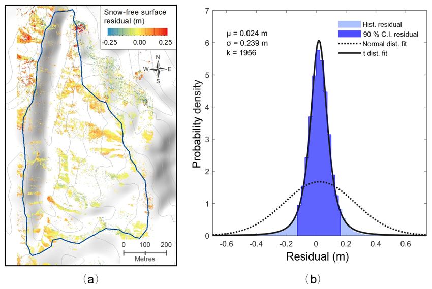
T. A. N. Redpath et al.: Repeat mapping of snow depth across an alpine catchment                                                      3481

Figure 2. Typical flight path for the mapping of the study catchment using the Trimble UX5, GCP network established for each flight mission,
and reference snow depth locations. Flight log is from the spring flight mission. The configuration of the ground control point (GCP) and
check point (CP) assignment for the triangulation of each flight is shown in the panels on the right-hand side.

greater than the expected accuracy of the models. Ground                tions. GNSS data were processed using Trimble Business
control networks were established for each RPAS flight mis-             Center (TBC) v3.40 software.
sion using real-time kinematic (RTK) GNSS surveying with                   It is well established that photogrammetric control is best
a Trimble R7 base station and R6 rover units. GCP locations             achieved within the bounds of the GCP network (Linder,
were measured with accuracy of the order of ∼ 0.02–0.03 m.              2016), while the uncertainty associated with the geolocation
GCPs were signalled with 0.6 × 0.6 m mats painted with a                of resected points increases beyond the control network. To
high-contrast circular quadrant pattern for the autumn and              constrain the area within the study catchment for photogram-
winter flights. For the spring flight, chalk powder was used            metric processing, the GCP network was distributed around
with a stencil to mark the target directly on the snow sur-             the catchment perimeter, as well as through the central area
face, using the same pattern as for previous flights. The use           of the catchment. Additionally, the placement of GCPs on
of chalk powder eliminated the need to retrieve GCP targets             the valley floor and at mid-elevation within the catchment
following RPAS flights. All survey work, as well as produc-             ensured that the network also sampled the elevation range of
tion of deliverables from photogrammetry, was carried out               the catchment. An extensive GCP network was established
in terms of the New Zealand Transverse Mercator (NZTM)                  for the first flight with no snow on the ground, which per-
reference system. All RTK survey work utilised a base sta-              mitted the robustness of AT to be tested under different GCP
tion established on a common benchmark, established for                 scenarios, as discussed further in Sect. 3.2.1. This allowed
this project, the position of which was differentially corrected        the network to be refined and reduced in size for subsequent
with respect to nearby continually operating reference sta-             missions, a matter of practical importance when working in
                                                                        alpine areas during the winter. Control point networks for

www.the-cryosphere.net/12/3477/2018/                                                           The Cryosphere, 12, 3477–3497, 2018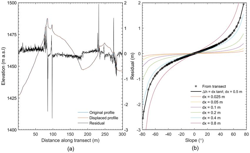
3482 T. A. N. Redpath et al.: Repeat mapping of snow depth across an alpine catchment
each mission are illustrated in Fig. 2. A new GCP network Brown (1971):
was established for each survey campaign due to the inabil-
ity to establish permanent markers (e.g. on poles) due to the x 0 = 1 + K1 r 3 + K2 r 5 + K3 r 7 x + 2T1 xy + T2 r 2 + 2x 2
conservation status of the study area. Although the layout of (1)
the network was similar for each mission, there were no com-
mon GCPs shared between different flights, with the only y 0 = 1 + K1 r + K2 r + K3 r y + 2T2 xy + T1 r + 2y 2 ,
3 5 7 2
common setting being the set-up of the base station for each
RTK survey. in which K terms are the radial distortion coefficients, T
terms are the tangential distortion coefficients, and
3.1.4 Reference snow depth measurements
x = x − x0 (2)
To assess the quality of snow depth data derived from RPAS y = y − y0 (3)
photogrammetry, independent measurements were collected q
by manual snow probing on 10 September 2016, the same r = x2 + y2. (4)
day as the spring RPAS mission. This approach has been es-
Image coordinates corrected for lens distortion are then used
tablished as standard practice in similar studies (e.g. Nolan
in the set of collinearity equations relating object point coor-
et al., 2015; De Michele et al., 2016). Aluminium avalanche
dinates (XA , YA , ZA ) to the corresponding image point coor-
probes with 0.01 m graduations, providing a nominal preci-
dinates (x 0 A , y 0 A ) to solve for the exterior orientation (Vander
sion of 0.01 m, were used. The sampling strategy involved
Jagt et al., 2015; Linder, 2016):
the measurement of snow depth every 50 m along three eleva-
tion contours within the study catchment, namely 1460, 1500
x0A
and 1540 m (Fig. 2). This strategy ensured that snow depth = (5)
y0A
was measured across a representative sample of slope aspect r (X − X ) + r (Y − Y ) + r (Z − Z )
and elevation, while optimizing navigation across the catch- 11 A 0 12 A 0 13 A 0
f
ment. Snow depths were measured at each location by prob- r31 (XA − X0 ) + r32 (YA − Y0 ) + r33 (ZA − Z0 )
r (X − X ) + r (Y − Y ) + r (Z − Z ) .
ing 5 times within arm’s reach, and the location of the central 21 A 0 22 A 0 23 A 0
f
measurement was surveyed with RTK GNSS, under the same r31 (XA − X0 ) + r32 (YA − Y0 ) + r33 (ZA − Z0 )
protocol and achieving the same level of accuracy as the GCP (X0 , Y0 , Z0 ) are the coordinates of the perspective centre of
survey. This provided 430 measurements of snow depth, with the image frame in the ground coordinate system. The rij
the mean snow depth at each of the 86 locations providing a terms represent the 3 × 3 rotation matrix relating the sensor
sample for comparisons with RPAS-derived snow depth. coordinate system orientation to the ground coordinate sys-
tem. Since the UX5 camera is fixed with respect to the plat-
3.2 Data processing form, the latter combines the roll, pitch and yaw (ω, ϕ, κ) of
the platform at the time of exposure. The nature of bundle-
3.2.1 Photogrammetric processing block adjustment with camera self-calibration dictates that
the quality of the final photogrammetric model is highly sen-
The goal of aero-triangulation (AT) in photogrammetry is sitive to errors in both sensor position and orientation as well
to transform a set of images into a scene in which geo- as inaccurate refinements of the interior orientation parame-
metrically accurate measurements can be made in three- ters (Ebner and Fritz, 1980).
dimensional, often geographic, space. This georeferencing
process requires a transformation from the inherent coordi- 3.2.2 Software and workflow
nate system of the device capturing imagery (a camera) to
an appropriate geographic coordinate system (Vander Jagt et Initially, AT was carried out using the photogrammetry mod-
al., 2015; Linder, 2016). While traditional photogrammetry ule of Trimble Business Center, v3.40 (TBC), which relies on
has long relied on metric (calibrated) cameras, the use of a simplified implementation of the adjustment process from
off-the-shelf non-metric cameras requires the simultaneous Inpho UAS Master. Deliverables produced using TBC, how-
solving of both interior orientation (the camera model) and ever, suffered from severe elevation artefacts which limited
exterior orientation. This process, known as self-calibration, their usefulness for further analysis. This is discussed further
applies a bundle-block adjustment to solve the camera model in Sect. 5.3.
describing the precise focal length (f ), the offset between Following the identification of shortfalls in TBC, AT was
the principal point of autocollimation and the centre of the carried out using Trimble Inpho UAS Master® v8.0 (UAS
imaging sensor plane (x0 , y0 ), and the departure between the Master). UAS Master is a feature-rich photogrammetry pack-
image point coordinate (x, y) and the idealized linear projec- age that is targeted to RPAS applications (Trimble, 2015,
tion due to lens distortion. Camera calibration parameterises 2016) and is a comprehensive alternative to software often
radial and decentering distortion with models such as that of used in similar studies such as Pix4D or Agisoft Photoscan.
The Cryosphere, 12, 3477–3497, 2018 www.the-cryosphere.net/12/3477/2018/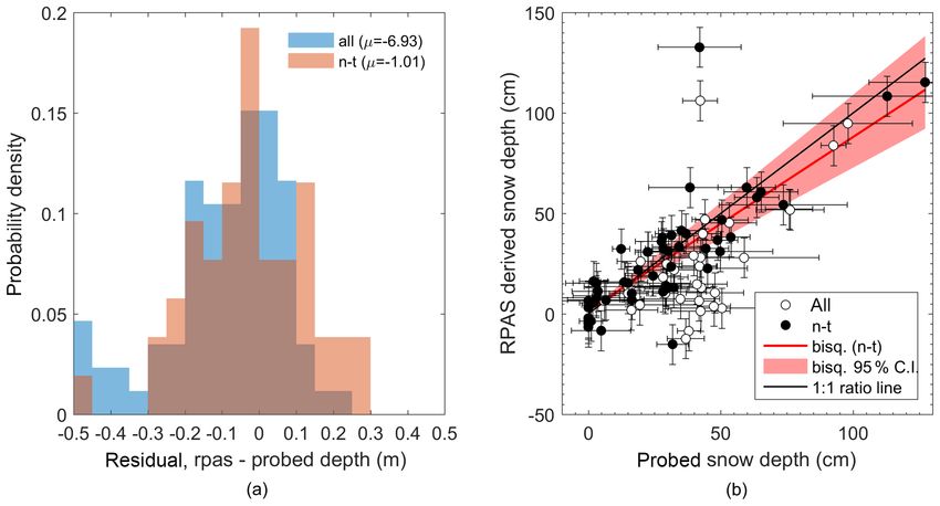
T. A. N. Redpath et al.: Repeat mapping of snow depth across an alpine catchment                                                    3483

Table 2. Summary results of alternative ground control point (GCP) and check point (CP) scenarios tested for aero-triangulation within UAS
Master.

                                                GCP RMSE (m)                           CP RMSE (m)
                            Scenario     n         x         y          z      n         x        y         z
                            1           23    0.0069    0.0076    0.0055      0         N/A      N/A      N/A
                            2           14    0.0017    0.0010    0.0004      9      0.0119   0.0184   0.0320
                            3            6    0.0033    0.0039    0.0009     17      0.0263   0.0207   0.0575

The AT solution is initialised by the positional parameters            3.2.3       Intermediate deliverables
(X0 , Y0 , Z0 ) for each photo centre, as provided by the on-
board GPS receiver. Relative adjustment is achieved after              Standard deliverables from the photogrammetric modelling
automatic tie point (TP) collection. TPs are common targets            included a dense point cloud; a digital surface model, inter-
recognised in multiple overlapping images, which allow the             polated to 0.15 m spatial resolution; and an ortho-mosaic,
relative position and orientation of images within the block           resampled to 0.05 m spatial resolution. The DSM and the
to be determined. Subsequent measurement of GCP positions              ortho-mosaic are the principal products for further analysis.
in images enables absolute adjustment. GCPs may be col-                Each DSM provides the basis for determining snow depth,
lected manually or automatically via feature recognition. In           while the ortho-mosaics allow for assessment of the snow-
this case, targets marking GCPs were identified and selected           covered area, and for snow-free areas to be identified when
manually. The absolute bundle-block adjustment then con-               assessing the quality and repeatability of DSMs between
currently refines the exterior and interior orientation param-         flight missions.
eters.
   The robustness of photogrammetric modelling was as-                 3.2.4       Derivation of snow depth
sessed by testing several alternate control scenarios, based
on the autumn mission when 23 GCPs were placed and mea-                Snow depth was derived by differencing DSM of flights 2
sured in the field. The following scenarios were evaluated:            and 3 from the baseline obtained during flight 1 (ref) as fol-
                                                                       lows:
  1. all 23 control points as horizontal and vertical GCPs,
                                                                       dDSMn = DSMn − DSMref .                                        (6)
  2. 14 control points as horizontal and vertical GCPs,
                                                                       Equation (6) provides a map of difference between the two
  3. 6 control points as horizontal and vertical GCPs.                 DSMs, henceforth referred to as the dDSM (after Nolan et
                                                                       al., 2015). Values of the dDSM are considered to represent
   In each scenario, the balance of the control points was             snow depth, with the associated uncertainty considered in
provided as check points (CPs). In retaining GCPs, we en-              Sect. 3.3.
sured that the perimeter of the study catchment remained
fully constrained within the network. As the number of GCPs            3.3     Quality and accuracy assessment
decreased, the root mean square error (RMSE) for CPs pro-
vided an indication of AT robustness. It was found that as few         Summary statistics, typically based on the rms error of GCPs
as 14 GCPs provided an acceptable triangulation across the             and CPs from the AT, indicate the expected accuracy of de-
study area, with some degradation apparent when only six               liverables. Since snow depth is determined by differencing
GCPs were used, primarily in terms of z (Table 2). No spa-             two DSMs, error propagation can provide an assessment of
tial structure was evident in the distribution of GCP or CP            uncertainty associated with the dDSM. The overall accuracy
error. This assessment aided the determination of an optimal           of the DSM differencing approach should also be validated
number of GCPs to minimise the time required to place and              against independent reference data (e.g. snow depth mea-
survey control points when snow is present in the catchment.           sured in situ), temporally coincident with RPAS measure-
On this basis, 14 control points were placed and measured              ments. Areas of snow-free terrain during Flight 3 further sup-
in the field for each of the winter and spring missions. For           plement snow depth observations by providing an extensive
all missions, the AT from which deliverables were produced             source of samples with which to assess the repeatability of
utilised all surveyed points as GCPs. A second AT was car-             the photogrammetric modelling process.
ried out using a subset of control points as CPs, as shown                Previous studies have considered the accuracy of RPAS-
in Table 3. Thus, the RMSE provided by CPs is expected to              derived snow depth by comparison with reference data from
be conservative compared to the quality of the deliverables            in situ snow depth alone (Bühler et al., 2016; De Michele et
obtained from the fully constrained AT.                                al., 2016; Harder et al., 2016) while ignoring the uncertainty

www.the-cryosphere.net/12/3477/2018/                                                           The Cryosphere, 12, 3477–3497, 2018
3484 T. A. N. Redpath et al.: Repeat mapping of snow depth across an alpine catchment
Table 3. Summary statistics for each of the triangulations used to produce DSMs and ortho-mosaics from each of the three flight missions
for ground control points (GCPs) and check points (CPs).
Flight n images n images GCP RMSE (m) CP RMSE (m)
captured used n TP n x y z n x y z
1 885 885 100 390 14 0.0083 0.0073 0.0034 9 0.0134 0.0163 0.0220
2 920 917 98 730 8 0.0067 0.0085 0.0018 6 0.0368 0.0293 0.0409
3 891 889 88 791 8 0.0105 0.0108 0.0028 6 0.0246 0.0247 0.0457
inherent to each photogrammetric model and their propaga- snow-free areas to characterise the experimental distribution
tion into the dDSM. Here, the accuracy of photogrammetri- of errors and assess the validity of the Gaussian assumption
cally derived snow depth is assessed by exploring both ap- in this context.
proaches. Relating photogrammetric model quality, as in-
ferred from GCPs and CPs, to observed uncertainties in the 3.3.2 Validation against reference snow depth
determination of snow depth provides the basis for realis- measurements
tically informing uncertainties in snow depth from ongoing
RPAS measurements. This in turn allows rigorous inferences The approach above provides a means to determine the ex-
about the evolution of snow depth to be made, without the pected accuracy of snow depth derived from RPAS pho-
need for further campaigns of in situ validation. While high- togrammetric surveys. In order to validate this estimate, a
resolution reference elevation data, such as lidar-derived ele- reference data set of in situ observations was sampled in
vation or surface models would provide a useful benchmark the field using snow probes, with a nominal precision of
for assessing RPAS DSM quality, no such data were available ±0.01 m, as described in Sect. 3.1.4. De Michele et al. (2016)
for the study area. assessed the accuracy of RPAS-derived snow depths against
snow depth surfaces interpolated from 12 point measure-
3.3.1 Uncertainty associated with RPAS-derived snow ments. This approach, however, may be limited by an inabil-
depth ity to accurately resolve the spatial variability of snow depth,
as well as the compounding effects of uncertainty associated
Since snow depth is determined via DSM differencing as with the interpolation scheme, particularly beyond the do-
a linear combination of two independently measured vari- main defined by the measured points.
ables (Eq. 6), the uncertainty associated with snow depth Here, 430 measurements of snow depth provided 86 mean
(SD), measured in the vertical dimension, for each measure- reference values, with the standard deviation of each set of
ment date (n) can be obtained via Gaussian error propagation five measurements providing 95 % confidence intervals. The
(James et al., 2012) as follows: aim of this sampling strategy was to assess and account for
q co-location uncertainty and spatial variability between the
εdDSM = εn2 + εref2 , (7) RPAS and reference snow depth data sets. Reference snow
depths were compared with those from the spatially coin-
where ε for each DSM is the elevation error determined from cident pixels from the map of RPAS-derived snow depth.
the AT as the RMSEZ value for the set of CPs. Inherent in RPAS-derived snow depth quality was assessed in terms of
this simple approach is the assumption that the planimetric residuals and weighted linear regression between reference
accuracy of each constituent DSM has negligible contribu- and RPAS-derived snow depths.
tion to εdDSM . Calculating εdDSM provides a single estimate
of uncertainty assumed to apply equally throughout the map 3.3.3 Repeatability of photogrammetric modelling
of RPAS-derived snow depth for each date. Under the as-
sumption that errors are normally distributed and bias-free, Emergence of snow-free areas at the time of the spring flight
the RMSEz derived from CPs identifies the standard devia- facilitated comparison between autumn and spring DSMs on
tion σz , allowing the 90 % confidence level of z to be deter- those areas. As the same terrain surface mapped from two in-
mined as 1.65×σZ . In turn, inferences associated with uncer- dependent flights should yield identical DSMs, the residual
tainties for elevation differences, εdDSM , also depend on the between them provides a means to characterise the distribu-
Gaussian assumption to provide the 90 % confidence level. tion of errors in the photogrammetric processing, which can
In reality, perfect co-registration between constituent be readily compared to the assessment made from CPs.
DSMs and the Gaussian assumption are unwarranted. Sub- Snow-covered and snow-free areas were segmented using
sequently, inferences associated with the evolution of snow an unsupervised classification of the spring ortho-image us-
depth may be compromised due to confidence intervals be- ing the Iso Cluster classification tool in ArcGIS v10.3. With
ing conservative or immoderate. Therefore, we use dDSM for five output classes, this approach enabled discrimination be-
The Cryosphere, 12, 3477–3497, 2018 www.the-cryosphere.net/12/3477/2018/T. A. N. Redpath et al.: Repeat mapping of snow depth across an alpine catchment 3485
tween illuminated snow pixels, shaded snow pixels, and veg- snow depths, despite the reduced control for subsequent ATs.
etation and soil-dominated snow-free pixels. Snow-free pixel For all flight missions, the photogrammetric processing per-
classes were then grouped to provide a mask within which formed well in the correlation of images and the construc-
the distribution of spring dDSM values could be character- tion of the image block, as indicated in Table 3. Tie point
ized. While this approach relies on the characterisation of (TP) generation relies on the successful match of unique tar-
repeatability for snow areas, good image contrast and the gets across multiple images, which was achieved despite the
high overall density of TPs generated across the image block, complicated contrast over snow. For all flights > 80 000, TPs
regardless of the presence or absence of snow, indicates were generated across the imaged area.
that photogrammetric reconstruction performance should be
comparable for both snow-free and snow-covered areas. This 4.1.2 Determination of snow depth
is a product of the camera properties, which maintain high
dynamic range across scenes of mixed land cover and exten- Snow depth was found to be highly variable across the study
sive snow cover. Therefore, this residual represents a mea- catchment for both winter and spring (Fig. 3). The mid-
sure of the repeatability of the technique for measuring sur- winter flight mapped near-complete snow cover across the
face height change, including derivation of snow depth. study catchment, while large snow-free areas developed by
the spring flight, where snow-covered area was reduced by
3.3.4 Resolution of fine-scale spatial variability about one-third (Fig. 3a and b). Where snow was present,
depths ranged from less than 0.10 m, typically on exposed
A primary motivation for exploring the use of RPAS pho- ridgelines and broad elevated slopes, to 2 m or more where
togrammetry for mapping a snowpack is the ability to re- cornices formed along ridgelines, as well as in gullies. Av-
solve fine-scale spatial variability in snow depth. This capa- erage snow depth was greater for winter, although maximum
bility was assessed by computing and comparing the semi- depths were comparable between winter and spring. Between
variograms of reference and RPAS-derived snow depths winter and spring, considerable ablation was observed. Ar-
from the autumn flight. While the sample size for reference eas of deepest snow were spatially coincident between win-
snow depths remained fixed (n = 86), the semi-variogram of ter and spring, with the greatest retention of snow in cornices
RPAS-derived snow depths could be calculated from many and gullies. Where shallow snow was present on ridgelines
more samples. Two random samples were extracted from the in winter, it was largely lost by spring.
spring dDSM map (n = 1000 and n = 5000), each yielding
a semi-variogram capturing the spatial variability of snow 4.2 Accuracy assessment and validation of snow depth
depth with increasing detail, which were compared to that
of the in situ observations. 4.2.1 Propagation of aero-triangulation error
Propagation of errors under the Gaussian assumption, based
4 Results
on the RMSE from each AT, yielded vertical uncertainties
4.1 Photogrammetric processing for snow depths at the 90 % confidence level of ±0.077 m
for the winter flight and ±0.084 m for the spring flight. This
4.1.1 Quality of the triangulation one-dimensional approach to error propagation assumes that
the planimetric geolocation of individual surfaces, and sub-
Since GCPs are used to solve the photogrammetric model, sequently the co-registration of surface pairs, does not con-
they do not provide an independent assessment of accuracy. tribute significantly to the vertical uncertainty.
Such an assessment is provided by the CPs, the RMSE of
which was of the order of centimetres for all flights (Ta- 4.2.2 Assessment against reference probe data
ble 3). Planimetric RMSE (i.e. x and y) was always sub-
stantially less than the GSD. Vertical RMSE (z) tended to Comparison of RPAS-derived and reference snow depth
be about double that achieved planimetrically but never ex- yielded a mean residual of −0.069 m, indicating that, on
ceeded 0.05 m. The final models were produced from a sec- average, reference depths were greater than RPAS-derived
ond and more constrained AT with all surveyed points used depths. Filtering the reference data set to exclude reference
as GCPs, thus making the assessment conservative relative to measurements that were made in areas occupied by tus-
the final products. sock (Chionochloa rigida) vegetation, however, improved
While the RMSE of CPs increased for the winter and the mean residual to −0.01 m (Fig. 4a). The small residual
spring flights, possibly due to a less constrained model, the is indicative of good agreement between the two data sets
level of accuracy achieved is compatible with expectations while also indicating that, overall, snow depths measured by
for the determination of snow depth. Additionally, the more probing may be overestimated. Limitations of probing and
tightly constrained first AT reduced the error for the baseline uncertainty introduced due to the presence of vegetation is
model, in turn contributing a reduced uncertainty in derived discussed further in Sect. 5.2.1.
www.the-cryosphere.net/12/3477/2018/ The Cryosphere, 12, 3477–3497, 20183486 T. A. N. Redpath et al.: Repeat mapping of snow depth across an alpine catchment
Figure 3. Processed ortho-mosaics for autumn (a), winter (b) and spring (c) flights, with corresponding autumn hill-shaded DSM (d) and
maps of snow depth derived for winter (e) and spring (f).
Good agreement between data sets is further demonstrated Table 4. Parameters of weighted regression between reference and
in Fig. 4b. Relatively large horizontal error bars accompany- RPAS-derived snow depths.
ing the reference measurements (Fig. 4b) reflect the substan-
tial spatial variability in snow depth measured by probing, n β0 β1 RMSE R2 p value
even within arm’s reach. Substantial departure occurs for ref- All points 86 0.92 0.80 14.7 0.67 0.000
erence snow depths between 0.20 and 0.60 m which tend to Non-tussock 52 1.69 0.86 11.3 0.82 0.000
exceed RPAS measurements. Negative depths in the RPAS-
derived data set is a product of co-registration uncertainty,
particularly in areas where the surface model represents large
vegetation or is influenced by rock outcrops, as well as spuri- derived and probed snow depths is likely due to the vary-
ous values from the constituent DSMs. Agreement between ing areas over which snow depth was sampled by the two
reference and RPAS-derived data sets improved with the re- techniques, and resulting spatial uncertainty in comparing
moval of reference measurements made above tussocks. This the two data sets.
filtering saw the R 2 value improve by 22 %, while RMSE
decreased by 23 % (Table 4). The 1 : 1 ratio line was con- 4.2.3 Comparison of DSMs from independent RPAS
tained within the 95 % confidence interval of the weighted flights
(bi-square) regression between RPAS-derived and filtered
reference snow depths. Some disagreement between RPAS The emergence of snow-free areas for the September flight
permitted a comparison of height derived on snow-free sur-
The Cryosphere, 12, 3477–3497, 2018 www.the-cryosphere.net/12/3477/2018/T. A. N. Redpath et al.: Repeat mapping of snow depth across an alpine catchment 3487
Figure 4. Residuals between snow depths measured by RPAS photogrammetry and probing for all probe locations (“all”, blue) and non-
tussock probe locations (“n-t”, red) (a), and bi-square (bisq.) weighted regression between snow depth derived from a 0.15 m RPAS grid
and probed snow depths (b). Vertical error bars are determined from the error propagation associated with DSM differencing and have
a magnitude of ±0.094 m, while horizontal error bars are calculated from the standard deviation of probe measurements made at each
reference sampling location.
Figure 5. Map (a) and histogram (b) of the vertical residual for snow-free areas for surface models derived from the autumn and spring
flights. The histogram includes fitted normal and t location-scale (t) distributions.
faces between the pre-winter and spring flights (Fig. 5). residual (bias) detected with respect to the pre-winter DSM
The small magnitude of the residuals, compatible with er- was 0.024 m (σ = 0.239 m) (Fig. 5).
rors consistent with the uncertainty of the triangulation CPs, The set of residuals departed substantially from the Gaus-
demonstrates the repeatability in the derivation of snow-free sian distribution and was better represented by the Student’s
surfaces. Furthermore, the absence of any spatially struc- t location-scale distribution (Fig. 6):
tured trend in the distribution of the residual indicates ro-
bust photogrammetric modelling from the RPAS platform.
! v+1
At 0.15 m resolution, the snow-free pixels from the spring 0 v+1
2 v + x−µ − 2
σ
f (x) = √ , (8)
σ vπ 0 v2
mission provided a large sample (n = 5 936 428). The mean v
www.the-cryosphere.net/12/3477/2018/ The Cryosphere, 12, 3477–3497, 20183488 T. A. N. Redpath et al.: Repeat mapping of snow depth across an alpine catchment
Table 5. Observed (calculated under Gaussian assumption) and fit-
ted normal and t location-scale (t l-s) parameters for the residual
distributions shown in Fig. 5b.
Parameter Distribution Value
Observed 0.024
µ (m) Normal fit 0.036
t l-s fit 0.019
Observed 0.239
σ (m) Normal fit 0.236
t l-s fit 0.056
ν t l-s fit 2.579
Figure 7. Comparison of histograms and accompanying descrip-
Figure 6. Mean, µ (a), standard deviation, σ (b) and distribution tive statistics for the residual between DSMs for slopes between 5
kurtosis (c) for the residual, in terms of discrete classes of slope (5◦ and 10◦ and slopes between 70 and 75◦ . Flatter slopes are found
width), up to the 90th percentile of slope. Kurtosis is plotted on a to exhibit extreme kurtosis relative to steeper slopes. Normal and t
log-scale and is accompanied by a standard error of 606. The slope location-scale (t) distributions are shown.
histogram has been clipped to the 90th percentile.
togrammetric modelling. Importantly, the significant depar-
where µ, σ and v are the location, scale and shape parame- ture from a normal distribution shows that assessing the vari-
ters, respectively. Large kurtosis (calculated k = 1956) asso- ability from a Gaussian fit on stable targets (±0.39 m at the
ciated with the histogram of residuals in Fig. 6 shows sig- 90 % level) would significantly overestimate the confidence
nificant departure from a Gaussian law (for which k = 3) interval. On the other hand, the 90% confidence interval cal-
of equal standard deviation, σ . The leptokurtic experimen- culated from the fitted Student’s t location-scale is ±0.10 m
tal distribution results in a narrower 90 % confidence inter- (Table 5). The significance of this result with respect to sta-
val than that estimated under the Gaussian assumption with tistical inferences is discussed further in Sect. 5.2.2.
σ = 0.24 m, while the probability of large residuals is larger The non-Gaussian nature of the residual distribution de-
than predicted by a Gaussian distribution. Overall, the mean serves further scrutiny. Similar distributions have been iden-
residual (µ = 0.02 m) and the precision of ±0.14 m (90 % tified for comparable repeatability assessments of pho-
confidence level, calculated from the distribution 90th per- togrammetric dDSMs used for mapping snow depth (Nolan
centile; Fig. 6) exceeds the uncertainties estimated from er- et al., 2015), but have not been explored in detail. Analysing
ror propagation alone (±0.08 m at 90 % confidence level; see the variability of the mean and standard deviation of the
Sect. 4.1.1) yet support the suitable repeatability of the pho- residual for discrete classes of slope, as well as the kurto-
The Cryosphere, 12, 3477–3497, 2018 www.the-cryosphere.net/12/3477/2018/T. A. N. Redpath et al.: Repeat mapping of snow depth across an alpine catchment 3489
Figure 8. Semi-variograms for snow depth, based on measurements provided by probing (86 samples), and two random samples drawn from
RPAS-derived snow depth of 1000 and 5000 observations.
sis of the residual distribution, provided insight into the role Table 6. Observed (calculated under Gaussian assumption) and fit-
of terrain. For classes of slope up to 65◦ the mean residual ted normal and t location-scale (t l-s) parameters for the residual
remains within the standard error, before becoming increas- distributions shown in Fig. 7.
ingly negative for the remaining classes (Fig. 6). Standard
deviation exhibits a similar trend, remaining largely within Slope class
the overall standard error for slope classes up to 45◦ , beyond Parameter Distribution 5–10◦ 70–75◦
which variability increases.
The observed pattern in the mean and standard deviation of Observed 0.026 −0.022
µ (m) Normal fit 0.026 −0.022
the residual indicates that larger and more variable errors are
t l-s fit 0.021 −0.118
associated with steeper slopes. Reduced kurtosis accompa-
nying the error distribution on larger slopes (Fig. 6) reveals Observed 0.186 0.892
a tendency towards a Gaussian distribution of residuals as σ (m) Normal fit 0.186 0.892
mean slope increases. Here, for slopes > 50◦ , kurtosis was t l-s fit 0.046 0.376
reduced below 100, and for slopes > 85◦ , kurtosis was less ν t l-s fit 4.104 2.093
than 10, approaching that of the normal distribution. There-
fore, the statistical distribution of error, while non-normal,
also varies significantly with terrain characteristics, as high-
lighted by the comparison of the residual histogram for dis-
crete classes of slope (Fig. 7 and Table 6). Subsequently, the Both the 1000 and 5000 random point samples captured a
overall distribution of residuals (Fig. 5b) is the result of a comparable structure of spatial auto-correlation with a range
convolution between non-normal distributions and the hyp- of ca. 40 m. The 5000-point sample improved the resolution
sometry of the area (i.e. area-elevation distribution). of the semi-variogram, with an improved signal-to-noise ra-
tio. In contrast, the reference data, despite being demanding
4.2.4 Characterising the spatial variability of snow in fieldwork, performed poorly at capturing the spatial vari-
depth ability, as most measurements were separated by a minimum
distance of 50 m. A lack of spatial auto-correlation in the ref-
The semi-variograms for RPAS-derived snow depth, com- erence data confirms a posteriori that probing samples could
pared to that from the reference measurements, are shown be assumed to be independent of each other, which is desir-
Fig. 8. They exemplify the new insight that high-resolution able for the accuracy assessment. Additionally, it also reveals
mapping provides into the spatial variability of snow depth. that probing failed to capture most of the spatial structure of
www.the-cryosphere.net/12/3477/2018/ The Cryosphere, 12, 3477–3497, 20183490 T. A. N. Redpath et al.: Repeat mapping of snow depth across an alpine catchment
the snow depth field, thus stressing a limitation of this clas- As identified by Nolan et al. (2015), photogrammetrically
sical method to characterise the snowpack. derived snow depths may also be affected by the compaction
of vegetation below the snowpack, which may introduce an
anomalous signal of surface height change, to the point of
5 Discussion returning false negative snow depths. Correcting observed
surface height change would not be straightforward, and is
5.1 Performance of RPAS photogrammetry for not possible with the data acquired within this study. The ef-
resolving snow depth fects of vegetation compaction are likely to be greatest in the
early winter. As grass typically does not rebound until after
Overall, RPAS photogrammetry is found to be suitable for
the complete removal of the winter snowpack, ongoing sub-
determining snow depth via DSM differencing. Primarily,
sidence of vegetation below the snowpack through midwinter
the achievement of uncertainties < 0.14 m at the 90 % con-
and spring is expected to be minimal. Ongoing future mea-
fidence level for derived snow depth, demonstrated empiri-
surement of snow depth via surface differencing (regardless
cally by the repeatability analysis (Fig. 5), provides a basis
of the source of DSMs) will benefit from the development
for useful data capture, and robust inferences and interpreta-
and incorporation of vegetation compaction and cavity mod-
tions. The reported magnitudes of uncertainties account for
els.
the sources discussed further below, and compare favourably
Ultimately, this study suggests that, for areas dominated
with other similar studies (Vander Jagt et al., 2015; Bühler
by tussock vegetation, RPAS photogrammetry may provide a
et al., 2016; De Michele et al., 2016; Harder et al., 2016).
more reliable means of measurement than probing. A lack of
Decimetre levels of uncertainty appear to be an emerging
knowledge regarding the specific location of sub-snow veg-
benchmark for snow depths measured by RPAS photogram-
etation when making measurements by probing is likely to
metry and also considered as standard for airborne lidar
provide a systematic overestimation of snow depth (Fig. 4).
(Deems et al., 2013). In terms of comparisons with in situ
In the New Zealand context, almost all seasonal snow oc-
data, Fig. 4 shows good agreement between RPAS and ref-
curs above the treeline, so the inability of photogrammetry
erence snow depth, and that RPAS photogrammetry perfor-
to penetrate the forest canopy is a lesser concern than for the
mance improves as snow depth increases. At the same time,
Northern Hemisphere.
use of probed snow depths as references for validating such
data can be compromised by the nature of the underlying
5.2.2 Geolocation and co-registration
vegetation.
Mapping snow depth continuously at 0.15 m resolution,
In mapping snow depth across a catchment with relatively
across an entire hydrological catchment, represents a new
complex terrain, we have been able to characterise the in-
contribution to the quantification and characterisation of spa-
fluence of terrain on dDSM uncertainty. The assumption
tial variability in snow depth on this scale, which is up to
that error associated with physical measurements is normally
2 orders of magnitude greater than many similar studies to
distributed and often underpins subsequent statistical infer-
date. Before considering the broader implications of this in
ences. As demonstrated in Sect. 4.2.3, the error associated
terms of snow processes, uncertainty, limitations and pitfalls
with the bias between independently acquired DSMs signif-
of the approach are considered.
icantly departed from normal and was better approximated
5.2 Sources and nature of uncertainty by the Student’s t location-scale distribution. This extremely
leptokurtic distribution of residuals reflects the influence of
5.2.1 Vegetation relatively low frequency, but high-magnitude residuals be-
yond the probability of the normal law, despite an overall
Vegetation contributes to uncertainty, particularly when val- dominance of residuals about and close to the mean. A pos-
idating RPAS-derived snow depths against reference snow sible source of large residuals between two DSMs is their
depths. As described in Sect. 4.2.2, the agreement between relative planimetric accuracy and subsequent co-registration
RPAS-derived and probed snow depths improved substan- quality (Kääb, 2005). For steep terrain in particular, a hori-
tially when areas of large tussock vegetation were excluded. zontal displacement between DSMs could add a component
It is likely that the presence of tussock introduces a bias into to dDSM uncertainty beyond the vertical accuracy of con-
the snow depth measurement, whereby a probe may penetrate stituent DSMs. The residual (1h) between two surface pro-
the tussock foliage, and possibly also a sub-vegetation void, files, which are identical but horizontally displaced by 0.5 m,
before striking the ground surface. This is similar to the cav- is shown in Fig. 9a. The error introduced to DSM differ-
ity effect highlighted for airborne lidar measurement of snow encing resulting from co-registration uncertainty increases
(Painter et al., 2016), and similar challenges have been docu- with steepening slope. Maximum residuals coincide with the
mented by Vander Jagt et al. (2015). High-resolution dDSMs, steepest terrain (near-vertical areas associated with rock out-
on the other hand, resolve the vegetation surface, and so veg- crops) and exceed 2 m. The sign of the error is aspect depen-
etation height is inherently better accounted for. dent, assuming a uniform horizontal displacement.
The Cryosphere, 12, 3477–3497, 2018 www.the-cryosphere.net/12/3477/2018/You can also read