Holographic topometry with high resolution for forensic facial reconstruction
←
→
Page content transcription
If your browser does not render page correctly, please read the page content below
Aus dem Institut für Lasermedizin
                 Direktor: Prof. Dr. Peter Hering

Holographic topometry with high resolution for
        forensic facial reconstruction

                       DISSERTATION

               zur Erlangung des Grades eines Doktors der
                              Zahnmedizin

        Der Medizinischen Fakultät der Heinrich-Heine-Universität
                              Düsseldorf

                              vorgelegt von

                              Frank Prieels

                             Dezember 2009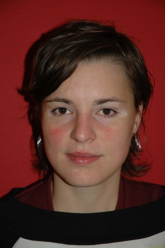
Contents                                                                                                                                                                            i

Contents

1 Introduction                                                                                                                                                                     2

2 The   human face                                                                                                                                                                 3
  2.1   Importance of the face     .   .   .   .   .   .   .   .   .   .   .   .   .   .   .   .   .   .   .   .   .   .   .   .   .   .   .   .   .   .   .   .   .   .   .   .   3
  2.2   Facial Recognition . .     .   .   .   .   .   .   .   .   .   .   .   .   .   .   .   .   .   .   .   .   .   .   .   .   .   .   .   .   .   .   .   .   .   .   .   .   3
  2.3   Facial Structure . . . .   .   .   .   .   .   .   .   .   .   .   .   .   .   .   .   .   .   .   .   .   .   .   .   .   .   .   .   .   .   .   .   .   .   .   .   .   4
        2.3.1 Skull . . . . . .    .   .   .   .   .   .   .   .   .   .   .   .   .   .   .   .   .   .   .   .   .   .   .   .   .   .   .   .   .   .   .   .   .   .   .   .   4
        2.3.2 Soft Tissue . .      .   .   .   .   .   .   .   .   .   .   .   .   .   .   .   .   .   .   .   .   .   .   .   .   .   .   .   .   .   .   .   .   .   .   .   .   8

3 Facial Reconstruction                                                                                                                                                            11
  3.1 History - overview . . . . . . . . . . . . . . . . . . . . . . . . . . . . . . . . . . . . . .                                                                               11
  3.2 Soft tissue measurement . . . . . . . . . . . . . . . . . . . . . . . . . . . . . . . . . . .                                                                                17
  3.3 Problems - difficulties . . . . . . . . . . . . . . . . . . . . . . . . . . . . . . . . . . . .                                                                              19

4 Holography                                                                                                                                                                       21
  4.1 Introduction - history       .   .   .   .   .   .   .   .   .   .   .   .   .   .   .   .   .   .   .   .   .   .   .   .   .   .   .   .   .   .   .   .   .   .   .   .   21
  4.2 Preceding works . . . .      .   .   .   .   .   .   .   .   .   .   .   .   .   .   .   .   .   .   .   .   .   .   .   .   .   .   .   .   .   .   .   .   .   .   .   .   21
  4.3 Holographic principle .      .   .   .   .   .   .   .   .   .   .   .   .   .   .   .   .   .   .   .   .   .   .   .   .   .   .   .   .   .   .   .   .   .   .   .   .   22
  4.4 Holographic camera .         .   .   .   .   .   .   .   .   .   .   .   .   .   .   .   .   .   .   .   .   .   .   .   .   .   .   .   .   .   .   .   .   .   .   .   .   23
  4.5 Optical reconstruction       .   .   .   .   .   .   .   .   .   .   .   .   .   .   .   .   .   .   .   .   .   .   .   .   .   .   .   .   .   .   .   .   .   .   .   .   25

5 Computed Tomography                                                                                                                                                              30
  5.1 Introduction . . . . . . . . . . . . . . . . . . . . . . . . . . . . . . . . . . . . . . . . . .                                                                             30
  5.2 Segmentation of CT data . . . . . . . . . . . . . . . . . . . . . . . . . . . . . . . . . .                                                                                  32

6 Experiment - probands                                                                                                                                                            34
  6.1 Introduction . . . . . . . . .           .   .   .   .   .   .   .   .   .   .   .   .   .   .   .   .   .   .   .   .   .   .   .   .   .   .   .   .   .   .   .   .   .   34
  6.2 Set up experiment . . . . .              .   .   .   .   .   .   .   .   .   .   .   .   .   .   .   .   .   .   .   .   .   .   .   .   .   .   .   .   .   .   .   .   .   34
  6.3 Mobile holographic camera .              .   .   .   .   .   .   .   .   .   .   .   .   .   .   .   .   .   .   .   .   .   .   .   .   .   .   .   .   .   .   .   .   .   36
  6.4 Protocol low-dose CT . . .               .   .   .   .   .   .   .   .   .   .   .   .   .   .   .   .   .   .   .   .   .   .   .   .   .   .   .   .   .   .   .   .   .   38

7 Methods                                                                                                                                                                          40
  7.1 Introduction . . . . . . . . . . . . . . . . . . . . . . . . . . . . . . . . . . . . . . . . . .                                                                             40
  7.2 Soft tissue measurement . . . . . . . . . . . . . . . . . . . . . . . . . . . . . . . . . . .                                                                                40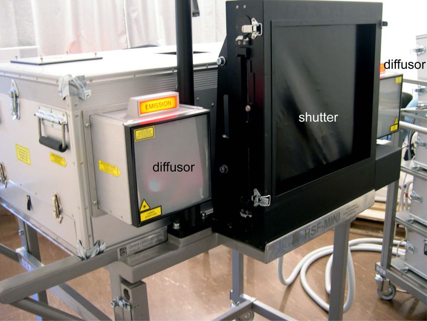
Contents                                                                                                     1

   7.3   Reproducability of the technique . . . . . . . . . . . . . . . . . . . . . . . . . . . . . .       44
   7.4   Results - evaluation . . . . . . . . . . . . . . . . . . . . . . . . . . . . . . . . . . . . . .   45

8 Problems - considerations                                                                                 54
  8.1 Segmentation of low-dose CT data . . . . . . . . . . . . . . . . . . . . . . . . . . . . .            54
  8.2 Soft tissue shift . . . . . . . . . . . . . . . . . . . . . . . . . . . . . . . . . . . . . . . .     55
  8.3 Tilted image . . . . . . . . . . . . . . . . . . . . . . . . . . . . . . . . . . . . . . . . . .      59

9 Conclusion                                                                                                60

Bibliography                                                                                                62
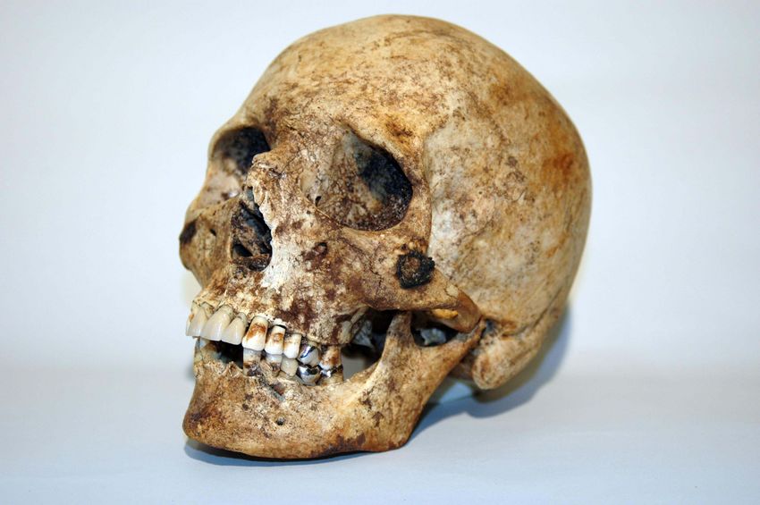
1 Introduction                                                                                          2

1 Introduction

Forensic facial reconstruction is a small field within the area of forensic medicine. Forensic odontolo-
gists, forensic anthropologists and specific trained artists are performing facial reconstructions. This
forensic technique can be useful when other identification methods fail.

Since more than 100 years, scientists are trying to measure the thickness of the facial soft tissue layer,
necessary to reconstruct a face. Measurements were performed both on living and dead persons. In
the early years, probes and needles were used to measure the soft tissue thickness. Later on, both
computers and ultrasonic equipment were introduced. Scientists faced some major problems though:
the number of facial measuring points were very limited and the measurements were not accurate.
Thus it was not possible to create a soft tissue database. On the other hand, there is a strong need for
a reliable database of facial soft tissue thickness in the medical and anthropological forensic world.

The aim of my research project was to develop an easy, efficient and reliable way to measure soft tissue
thickness of the face. We used a small number of probands, within the same subcategory (age, ethnic).
Holography was the perfect solution to reproduce the facial outline.

In order to develop a new technique to do high precision facial soft tissue measurements, it is necessary
to compare the holographic data to bone surface information. Computed Tomography can be a good
source to provide these data. It is the first time a technique is developed to do high precision facial
soft tissue thickness measurements, resulting in a dense field of measurement points.
2 The human face                                                                                        3

2 The human face

2.1 Importance of the face

The human face is an important social tool. We use our face to produce signals expressing emotion
and attention. Each face is unique. We are able to notice small variations between faces; this will help
us in recognizing and identifying persons. The morphology of the face provides us information about
age, health, ethnic group, gender...

The underlying skeleton affects the morphology of the face. The different shapes of the individual skull
bones provide a large variation between skulls.
The overlying soft tissue and secondary details such as skin colour, hair, ears, eye colour, wrinkles...
will determine the unique character of the face.

2.2 Facial Recognition

A human face reveals lots of information to a perceiver; it can tell about mood and intuition, but it can
also serve as an identification tool. Facial recognition is one of the most studied areas in psychology.
Still, the process of recognizing and other aspects of face processing were described by Bruce et al
[RE1]. They presented a theoretical framework for face recognition. They argued that there are at
least seven distinct types of information that can be derived from faces. In facial recognition, two
codes are involved in face processing: the pictorial code and the structural code.

A pictorial code is a description of a picture. It is a more abstract level, and it can be used to make
yes/no recognition memory decisions. Structural codes give us the ability to distinguish a face from
other faces. Codes for familiar faces differ from those formed to unfamiliar faces. The recognition of
unfamiliar faces is not simple. And it is well documented that most people find it easier to memorise,
interpret and recognise faces of persons belonging to their own racial group ([RE2] Shepherd, 1981;
[RE3] Wilkinson). This is called the ’other-race’ effect. For example, hair colour can be a distinguishing
factor among caucasians, it is not the case in a black or asian population. It is however described that
increased contact with a different racial group will improve performance of recognition in that racial
group ([RE4] Mc Kelvie, 1978; Shepherd, 1981).
2.3 Facial Structure                                                                                   4

2.3 Facial Structure

2.3.1 Skull

The skull is the term used to name the bonal framework of the head. It is the most complex part of
the skeleton as it protects and supports both the brain as well as the organs of sight, smell, taste and
hearing.

It is of major importance for physical anthropology . The skull develops under the influences of tension,
maturation and growth.

Some knowledge of the correct cranial terminology is important when assessing the skull:

   • Skull: the entire skeletal framework of the head.

   • Cranium: the skull minus the mandible.

   • Calvarium: the cranium minus the face.

   • Mandible: the lower jaw.

   • Splanchnocranium: the facial skeleton.

   • Neurocranium: the brain case.

There are 22 bones in the skull: 6 unpaired and 8 paired; 14 facial bones and 8 cranial bones. Although
the hyoid is often grouped with the skull, it is usually not considered a part of it. The bones of the
skull unite along serrated joints known as sutures. Most sutures take their names from the two bones
of the skull that go together to form the suture. But there are 5 exceptions to this rule:

   • coronal suture: between frontal and parietals.

   • Sagittal suture: between the two parietals.

   • Lambdoidal suture: between parietals and occipital.

   • Baselar suture: between sphenoid and occipital.

   • Squamosal suture: between parietal and temporal.
2.3 Facial Structure                                                                                   5

Description of the bones of the skull:

                                     Figure 2.1: Bones of the skull.
                                          Left: frontal view.
                                          Right: lateral view.

Frontal bone: forms the forehead and the upper part of the orbital cavity. Important is the supra-orbital
ridge, a prominence above the orbits, often seen in males.

Parietal bones: compose part of the top and the sides of the cranium, posterior of the frontal bone.

Temporal bones: form the lower, lateral sides of the cranium.

Occipital bones: form the back and the base of the cranium. Not so important in facial forensic
reconstruction.

Nasal bones: join the maxillae and the frontal bone.

Maxillae: form the upper jaw.

Zygomatic bones: forms the prominence of the cheek, and can be felt under the skin just below and
lateral to the eye socket.

Mandible: separate bone, hinged to the cranium at the temporomandibular joint. The mandible has
three important parts: the ramus, the condyle and the coronoid process.

Description of the common cranial landmarks:

Alare (al): the most lateral point on the margin of the nasal aperture.

Bregma (b): the cranial point where the coronal and sagittal sutures intersect.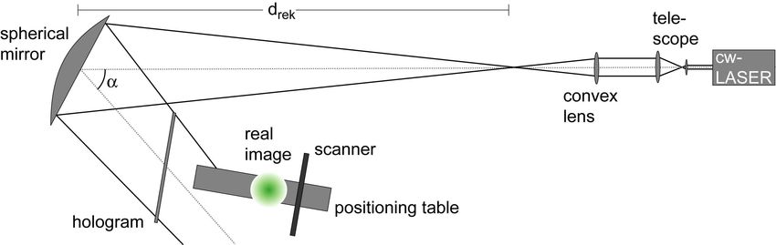
2.3 Facial Structure                                                                                    6

Coronium (cr): point at the top of the mandibular coronoid process.

Ectoconchion (ek): the most lateral point on the orbital margin.

Euryon (eu): the cranial point at the greatest cranial breadth.

Glabella (g): the most prominent point between the supra-orbital ridges in the midsagittal plane.

Gnathion (gn): the most inferior midline point on the mandible.

Gonion (go): point at the centre of the mandibular angle.

Incision (inc): point where the central incisors meet on the incisal line.

lambda (l): intersection of the sagittal and lambdoidal sutures in the midplane.

Mentale (ml): the most inferior point on the margin of the mental foramen.

Metopion (m): cranial midline point on the frontal bone where the elevation of the curve is greatest.

Nasion (n): midpoint of the suture between the frontal and the two nasal bones.

Nasospinale (ns): midline point of a tangent between the most inferior points of the nasal aperture.

Opisthocranion (op): the midline cranial point on the occipital bone, most distant from the glabella.

Orbitale (or): most inferior point on the orbital ridge.

Pogonion (pg): most anterior midline point on the skin.

Porion (po): the uppermost point on the margin of the external auditory meatus.

Prosthion (pr): most anterior midline point on the alveolar process of the maxilla.

Rhinion (rhi): midline point at the inferior end of the internasal suture.

Vertex (v): highest midline cranial point on the zygomaticomaxillary suture.

Zygion (zy): most lateral point on the lateral surface of the zygomatic arch.
2.3 Facial Structure                                                                                 7

Sex determination of the skull:

Due to the influence of interpopulation variation, sex determination from the skull alone may be
problematic; there is a certain overlapping of the two sexes. Stewart [SK1] showed he could determine
the sex of an entire adult skeleton with 90-95 % accuracy, and 80 % for the skull alone. He also stated
that female measurements are 92 % of the male measurements.

Krogman and Iscan [2D2] investigated 750 skeletons and had 100 % success rate when sexing the entire
skeleton, 95 % with pelvis alone, and 92 % with skull alone. It should however be pointed out that the
male/female ratio of the specimens investigated was about 15/1.

Absolute differences seldom or never exist, and many intermediate skull forms do exist. Krogman
and Iscan [2D2], White and Folkens [SK2] and Iscan and Helmer [SK3] did find some distinguishing
characteristics. The female skull is generally smaller, smoother and more gracile than the male. The
forehead contour in the female is higher, more rounded, more vertical and smoother than in the male.

Supra-orbital ridges are more prominent in males than in females (fig. 1.2). The glabellar region is
larger in the male. Female skulls have sharper orbital margins, the orbits are higher and more rounded.
Muscle ridges, especially on the occipital bone, are larger in males. Also the mastoid processes are
larger in males. The male mandible has a greater body height, is larger and thicker.

                              Figure 2.2: Sex determination of the skull.
                                 Left: male skull. Right: female skull.

These variations in skulls lead to differences between male and female faces. Enlow [SK6] pointed out
that the male face is typically larger, with a larger and more protrusive nose, and more deep-set eyes.
Typical is the bulging glabella and the supra-orbital ridges.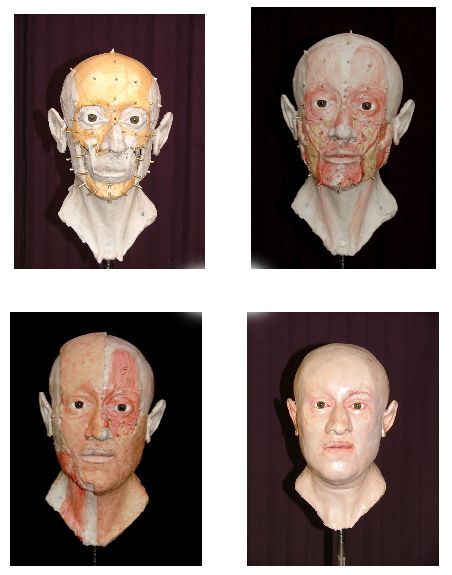
2.3 Facial Structure                                                                                       8

Race estimation of the skull:

The skull is the only area from the skeleton from which an accurate race estimation may be obtained.
Nevertheless, it is a difficult assessment to determine the racial affiliation; classifying groups on the
basis of facial appearance is not evident - Sauer [SK4], Brothwell [SK5].There is some genetic mixing,
due to migrating populations around the world. Secondly, there are overlaps between different racial
groups, and thirdly there is much variation within the same racial group. The most common racial
groups are Caucasoid, Negroid and Mongoloid.

     CAUCASOID skull                   NEGROID skull                   MONGOLOID skull
     long, narrow shape                long head shape                 round head shape
     narrow nasal opening              wide nasal aperture             medium-width nasal aperture
     little or no prognathism          strong alveolar prognathism     moderate prognathism
     depressed nasal root              low rounded nasal root          short nasal spine
     moderate supra-orbital ridge      sharp upper orbital ridge       no brow ridges
     narrow interorbital distance      wide interorbital distance      wide facial breadth
     depressed glabella                rounded glabella                prominent zygomatic bones
     large mastoid processes           bregmatic depression            flatter face

2.3.2 Soft Tissue

The skull is covered by a soft tissue layer, consisting of fat, muscles, vessels, salivary glands, nerves and
skin (fig. 2.4). The facial outline is mostly determined by the musculature and fat. Because muscles
control expressions of the face, they are sometimes referred to as muscles of "facial expression". They
also act as sphincters and dilators of the orofices of the face (i.e. orbits, nose and mouth).

Facial muscles can be divided in 4 groups:

   • orbital group

   • nasal group

   • oral group

   • other

Gerasimov (1971) [FR12] stated that when reconstructing a face, the artist / scientist should have
a deep understanding of the muscles of the face and neck, their attachments, origins and actions.
Research into facial soft tissue through dissection will allow an anatomically correct facial outline (fig.
2.5).
2.3 Facial Structure 9
Figure 2.3: Race stereotypes of the skull.
a) caucasoid skull. b) negroid skull. c) mongoloid skull.2.3 Facial Structure 10
Figure 2.4: Muscles of the head. Image source: Richard Neave.
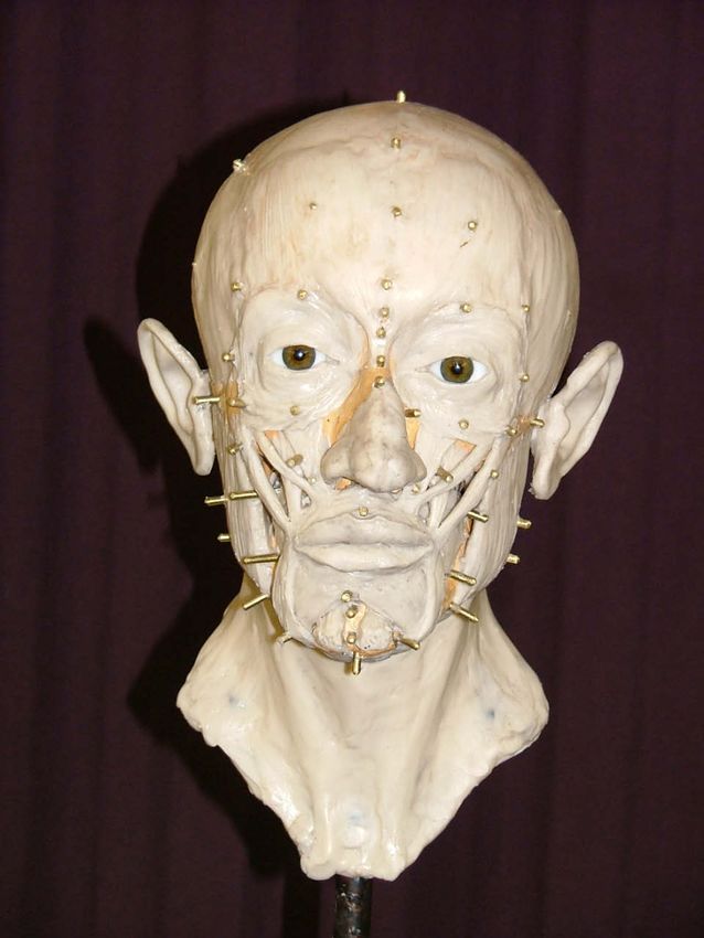
Figure 2.5: Facial muscles and markers, showing main tissue depth at specific anatomical points, in an in-
termediate stage of a plastic reconstruction, according to the Manchester method. Image source: Richard
Neave.3 Facial Reconstruction 11 3 Facial Reconstruction 3.1 History - overview Facial reconstruction, the scientific art of visualising faces on skulls for the purpose of identification, has been exercised for over a century. Scientific art is the use of artistic skills following scientific rules. Within forensic anthropology, facial reconstruction is used when all other alternatives are unsuccessful. The technique is indicated when dealing with burnt, severely mutilated, skeletonised or decomposed bodies or remains. The aim is to get a resembling image of the person prior to death. The reconstruction may be presented on television or in newspapers. Hopefully someone, somewhere will be able to identify the deceased. Anatomists in the late 19th century conducted much of the early research in facial reconstruction. There have been many applications of facial reconstruction in the past, including its use in the reproduction of busts from skulls of famous people. Faces of these historical people were created by comparing them with death masks and portraits in order to corroborate the authenticity of skulls found in tombs. Between 1867 and 1883, the German anatomist Welcker [HI1, HI2, HI3] used two-dimensional recon- structions to discuss the skulls and death masks of Dante, Schiller and Kant. He utilised tissue depths he had collected from cadavers. A variation of this method was used by His [HI4] in 1895, to reconstruct Johann Sebastian Bach’s face and compare it to the portraits of the composer that were available. In that period, faces were categorised according to the tissue thickness; average male, average female, and maximum-minimum variations for both sexes. In 1898, Kollman and Büchly [HI5] made a modelled reconstruction of a prehistoric skull, using tissue depth markers and clay. They also compared their results with those of His, and combined the data to obtain mean values, and maximum-minimum variations. It is generally recognised that there are three different techniques for facial reconstruction: 1. two-dimensional facial reconstruction (2D) 2. video superimposition
3.1 History - overview                                                                                 12

  3. three-dimensional facial reconstruction (3D)

1. 2D-facial reconstruction

In the 2D-facial reconstruction, an artistic drawing is placed over the representation of the skull. This
reconstruction method creates a face from the skull with the aid of soft tissue depth estimates. In
1977, Cherry and Angel [2D1] produced a drawing of the face by using a skull photograph. Krogman
and Iscan [2D2] used lateral and frontal radiographs to make tracings (1986). Also George [2D3] used
lateral radiographs; he mentioned this data set could be important for calculating facial profiles (1987).
Ubelaker [2D4] developed a technique, using soft tissue thickness markers on the skull. A photograph
is then taken in the Frankfurt plane. Later, computer-assisted approaches to facial reconstruction
became more popular. In 1992, Ubelaker and O’Donnell [2D5] described the F.A.C.E.™ system, which
is a a two-dimensional computerised and digitised version of Ubelaker’s earlier work. The C.A.R.E.S.™
system also produces composite images, as the result of an overlay of both a photograph and a sketched
image, using contours of the skull. The advantage of these computerised systems is that they can
produce different composite images from the same skull contour, by using different facial features.

                       Figure 3.1: Different features of one basic composite picture.
3.1 History - overview 13 2. video superimposition The technique of video superimposition is used to compare the skull with a pre-mortem photograph; it is an attempt to supply a face for a found skull. The purpose is to establish a close enough relationship between the two images, to state that these belong to the same individual, with a high degree of confidence. The first image is that of the unidentified skull. The image of the face can be derived from a photograph (most common), or from radiographs. One of the difficulties of superimposition is the orientation of the skull to the image of the face. Iten [FR1] related the eye level to the external auditory meatus, in order to determine the anterior-posterior tilt. Seta and Yoshino [FR2] mounted the skulls and adjusted the orientation using a joystick. Smeets and Prieels used a combination of relation between the eye level l external auditory meatus (fig. 2.3). A robot can digitally move over 6 different axes, in order to get the exact position of the skull. Two video cameras are mounted and fixed; one camera is recording the photograph, the other one is recording the skull. All movements should be recorded digitally, to make the investigation work reproducible (fig. 2.2). If we want to match the skull and face image correctly, both should have the same size. Maat [FR4] searched on the positioning and magnification of skulls and faces. The validity of superimposition techniques has always been a point of discussion. Cocks [FR5] compared triangulated anthropological points marked on the skull and on the face photograph, to quantify the comparison. Brown [FR6] argued that it is difficult to find the points on a face photograph. In a study on 52 European skulls, Helmer [FR7] concluded that skulls were comparable in their in- dividuality to fingerprints. In his work, Helmer defined 34 distinctive points on the skull, which very often serve as the reference (Helmer points) [SK3]. De Vore [FR8] pointed out that photographic superimposition is of better use in exclusion rather than inclusion. Brown [FR9] reported that Australian courts accept video superimposition as an identification method.
3.1 History - overview                                          14

Figure 3.2: Skull mounted on robot.
  Video superimposition technique used by Smeets and Prieels.
  Image source: Bregt Smeets (on unpublished work)
3.1 History - overview                                                            15

                Figure 3.3: Superimposition of a picture over an unknown skull.
3.1 History - overview 16 3. 3D-facial reconstruction Several methods exist which utilise soft tissue depth markers fixed to the skull or a cast. The soft tissue of the face are then built up with clay, plasticine or wax. The method is dependent on the knowledge of certain features of the skull, as well as the use of tables of mean values of facial soft tissue thickness, measured at some specific landmarks. Neave [FR10] said that it is often a collaboration between the anthropologist and the artist, where the artist works using instructions from the anthropologist. Normally the reconstruction is made on a copy of the skull, to avoid any damage to the skull; it can be a plaster model or a rapid prototyping model. In case of a plaster model, an alginate impression is taken of the skull. Both skull and mandible are fixated in a central relation (rest position of the two jaws without occlusion). They can be fixed using dental wax. The choice of tissue depth data is determined by sex, age and ethnic origin of the skull. Holes are drilled into the model , rectangular to the model surface. Markers (rubber or wooden pegs) are cut off to the length according to the soft tissue thickness at that specific landmark, and fixed to the model. The Russian anthropologist Gerasimow was a pioneer in developing the Russian or anatomical method of three-dimensional reconstruction. The face was rebuilt muscle by muscle, without the use of tissue depth measurements. He believed there was a correlation between details of nose, eyes, mouth, ears, and the relief of the skull at specific areas [FR12]. The following subcategories of 3D facial reconstruction exist: 3-1: strip plastic facial reconstruction. In this technique, strips of clay are used to fill up the spaces between the landmarks. The skin is formed by filling in any gaps and smoothing the whole surface [FR11]. The disadvantage of this method is that the surface information between landmarks remains inaccurate. In areas with few landmarks, this may have an influence on the changes in contour over the soft tissue surface. Any interferences noticed from the skull, should be added to the reconstruction in a second step. 3-2: anatomical facial reconstruction As in the former technique, markers are placed to the landmark sites corresponding to tissue depth values, found in reference tables. The Manchester method of facial reconstruction is developed by Neave and Wilkinson [FR10]. Plastic eyeballs are positioned in the orbita. One by one, the muscles of the face are modelled on the skull. Position and form of these muscles are related to the shape and form of the face. The tissue depth pegs can act as a guide, but sometimes these pegs are misleading, according to the specific morphology of the skull. The reconstruction practitioner should keep in mind that the soft tissue thickness data are average tissue measurements that will not be accurate for an individual skull.
3.2 Soft tissue measurement                                                                             17

In the next stage, a layer of clay will reconstruct the subcutaneous fat and skin. Every detail of
the reconstructed face must be based on scientific assessment of the skull morphology. Hairstyles,
wrinkles, beard, scars and glasses should only be added if these are suggested according to the post-
mortem information provided by the forensic pathologist. False information may mislead the observer.
In contrast, Taylor [FR13] uses eye colour, skin tone etc from population statistics. In the Manchester
method, practitioners prefer to add only those facial features that are certain.

Figure 3.4: Different steps in anatomical facial reconstruction.
  Skull, muscles, fat, skin. Image source: Richard Neave.

3.2 Soft tissue measurement

Collecting data on facial soft tissue measurements is important in order to perform an adequate recon-
struction of the face. The first research into facial soft tissue depth was done by the early practitioners
of facial reconstruction. They provided their own tissue depth measurements. Welcker [HI3] carried
out the first documented research in 1883. He collected measurements from cadavers by sliding the
3.2 Soft tissue measurement                                                                       18

blade of a scalpel through the tissue at predefined landmarks. The blade was then marked and the
depth of the scalpel’s penetration was measured. He studied 13 white male cadavers of middle age. In
1895 His [HI4] used a modification of Welcker’s technique to obtain tissue depth information; he used
a needle pushed into the skin of the cadaver, which displaced a rubber disc, representing the depth.
Kollman and Büchly (1898 [HI5]) expanded on His’s research; they bused a needle, covered on soot,
with the clean area of the needle indicating the thickness of the soft tissue.
Other earlier research on soft tissue thickness was done by Czekanowski (1907 - [STM1]), Berger (1965
- [STM2]), Leopold (1968 - [STM3]), Suzuki (1948 - [STM4]).
In 1980, Rhine and Campbell [STM5] took measurements from Black American cadavers, they chose
unembalmed bodies (deceased no longer than 12 hours) to minimise post-mortem effect on the soft
tissue. Rhine and Moore (1982 - [STM6]) did a similar work, measuring tissue depths on White
Americans.

There are some problems with cadaver studies (ctr later); different and more accurate of soft tissue
thickness measurements were therefore studied.

One of the new techniques was to take different measurements from cranial radiographs. Research on
making soft tissue measurements on White Europeans was done by Bankowski (1958 - [STM7]) and
Leopold (1968 - [STM3]); Weining (1958 - [STM8]) and George (1987 - [2D3]) investigated craniographs
of White Americans.
A study of Aulsebroock (1996 - [STM9]) measured the faces of 55 male Zulus, using both radiographs
and ultrasound. Phillips and Smuts (1996 - [STM10]) studied 32 Mixed Race subjects using CT scans,
whilst Sahni (2003, [STM11]) took MRI scans of a population of 60 Indians.
Ultrasound was introduced as a safe and effective way to measure soft tissue thickness. Helmer (1984,
[STM12]) studied 123 White European subjects. The results were divided into ten-year interval age
groups and by sex.
Lebedinskaya and her team (1993 - [STM13]) studied 1695 individuals, from nine ethnic groups within
the former USSR.
De Greef (2005 - [STM14]) used an ultrasound-based system to measure soft tissue thickness of 967
Caucasians.
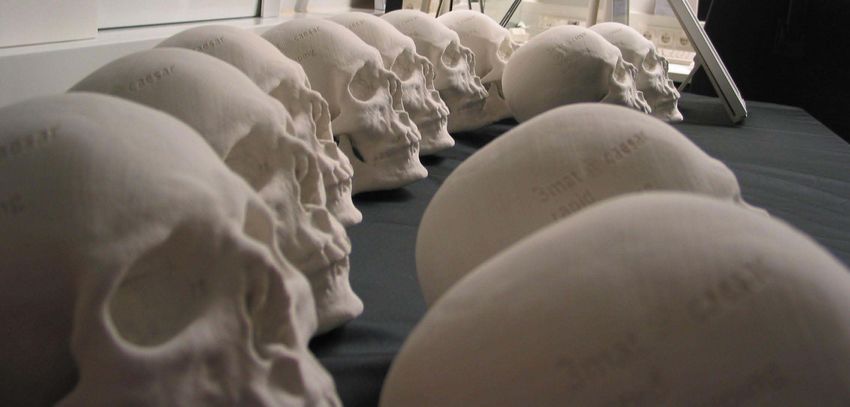
3.3 Problems - difficulties                                                                            19

3.3 Problems - difficulties

Not only the problem of accuracy of soft tissue depth data, but also the lack of understanding of
how soft tissue changes between the landmarks, make facial reconstruction widely criticised. Many
studies showed that the lack of accurate and comprehensive soft tissue depth data is one of the factors
contributing to the inaccuracy of facial reconstruction [FR14, FR15]. The problems regarding the soft
tissue depth data are both the mode of collection of the data, and the choice of landmarks. The results
of the cadaver measurements are not considered to be an accurate representation of the amount of
tissue on the face in a living person (shrinkage, loss of muscle tone, general signs of putrefaction). One
problem associated with the ultrasonic technique is the placing of the pen tip at the correct anatomical
point over the skull; it is not always simple to locate these points. Values of measurements also depend
on the angle of the needle or the ultrasound probe. A slight angle deviation can change the measuring
results dramatically. An additional problem is the lack of landmarks in some areas (e.g. cheek area);
this makes it difficult to find the right cheek contour [FR16].

These measurement datasets have further limitations; there is only a small number of subjects in the
soft tissue depth studies, and there are limited data available of different age, sex and race groups.

In preparation of the 2nd International Conference on Reconstruction of Soft Facial Parts in Remagen,
Germany (2005), participants were asked to perform a reconstruction on an unidentified skull (fig.
3.5). A Rapid Prototyping (RP) model of the skull - prepared by the CAESAR RP group - and a
report of the anthropological examination - done by the Institute of Anthropology of the University
of Goettingen - were presented to the participants (fig. 3.6). They had the choice between a drawing,
2D- and 3D-computer reconstruction and a sculpture.

The results were rather fascinating as they showed a large variation on reconstructions. The whole
experiment showed that both science and artistic skills will influence the result of a facial reconstruc-
tion.
3.3 Problems - difficulties 20
2nd International Conference on Reconstruction of Soft Facial Parts (Jens Bongartz, Remagen 2005).
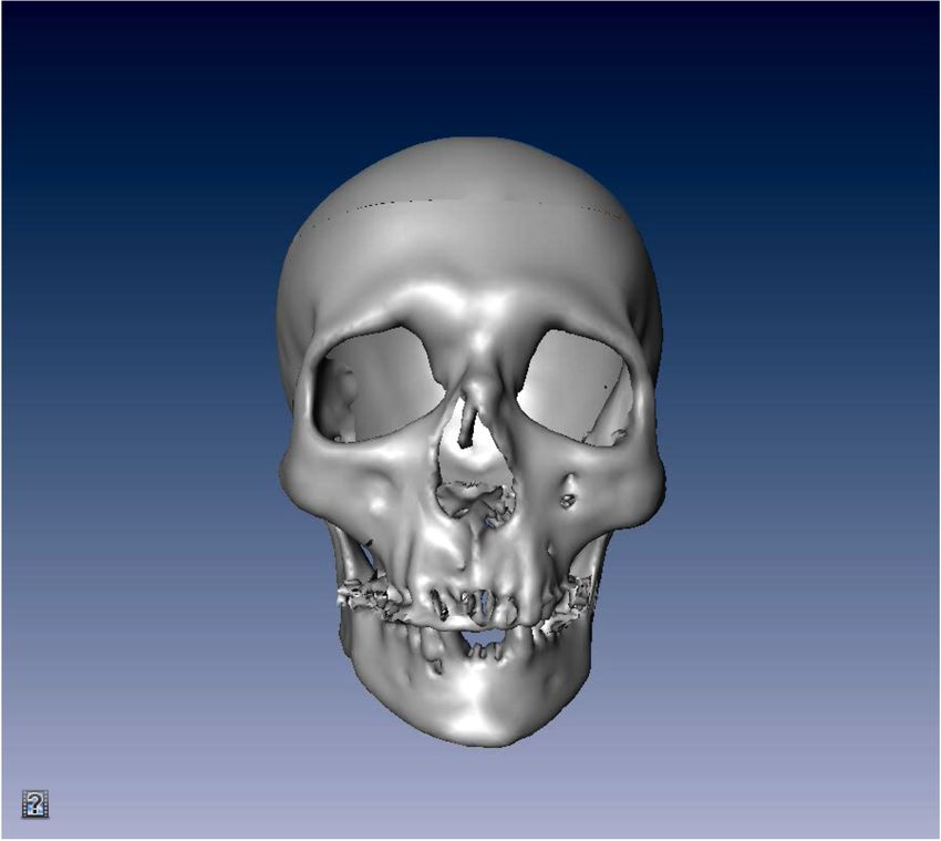
Figure 3.5: Left: unidentified skull.
Right: CT image unidentified skull.
Image source: Jens Bongartz.
Figure 3.6: Rapid Prototyping Replicas of the skull.
Image source: Jens Bongartz.4 Holography 21 4 Holography 4.1 Introduction - history Both in maxillofacial reconstructive surgery [Ho-In1] as in forensic soft tissue measurements, there is a strong need for a contact-free, optical measurement system. This requires a system with a good optical resolution and a short measuring time. Chen [Ho-In2] made an overview of a three dimensional shape measurement using optical methods. Bongartz [Ho-In3, Ho-In4] focused on this issue and stated that none of these techniques were useful for facial measurement; both exposure time and resolution did not meet the medical requirements. To fulfill the requirements for facial measurements of living persons, the Holography and Laser tech- nology group at CAESAR (Center of Advanced European Studies and Research) in Bonn developed a topometry system based on pulsed holography. Gabor [Ho-In5] invented the concept of holography in 1947, for which he was rewarded the Nobel Prize in 1971. In his historical demonstration of holographic imaging, a collimated beam of monochromatic light was used to illuminate a transparency consisting of opaque lines on a clear background. The interference pattern produced by the directly transmitted beam and the light scattered by the lines on the transparency were recorded on a photographic plate. Gabor wanted to use a lensless imaging system, as he found that the quality of the electron lenses was too poor. He recorded an electron wave field on a medium, and reconstructed it optically at a later time. He named the interference pattern optical holography, from the Greek holos (whole) and graphe (writing). Although this application of holography was never used in electron microscopy, the development of the laser led to optical holographic surfaces. 4.2 Preceding works In the Holography and Laser Technology Group (Prof. Hering) at the CAESAR foundation in Bonn, the use of analog portrait holography was introduced as a tool for facial topometry, using a short-pulsed green laser.
4.3 Holographic principle                                                                             22

The development and improvements of this approach were described in five PhD theses and in many
articles.

The first thesis on holographic facial measurement was written by Bongartz [Ho-In4]; he described the
advantages of the fast capture as an optimal tool for the measurement of faces of living persons. He
used a diffuser screen and a CCD camera to create the real image digitization. His work included the
whole holographic recording process, several medical considerations, as well as the scattering properties
of the skin.

Giel [Ho-In6] used inverse filtering and iterative deconvolution in conjunction with holographic real
images. He introduced a laser speckle projection to improve the skin contrast, and discussed the
influence of moving apertures and additional aperture by adding mirrors.

Frey [Ho-In7] used a CMOS flatbed scanner instead of a diffuser screen and a CCD camera, to digitize
the real image directly. The quality of the real image improved so much, that no further structured
illumination was needed. From now, eye-safe recordings were possible.

Thelen [Ho-In8] concentrated on contrast based methods for extracting three-dimensional information
from two-dimensional projections (surface extraction). She evaluated twelve different mathematical
operators for contrast measurement; the XSML (Extended Sum Modifies Laplacian) performed best.

Hirsch [Ho-In9] presented a full-sized area detector to replace the platbed scanner. Thus he eliminated
the shortcomings of speed, dynamic range, mechanical instability and image artefacts. This scanner
uses a X-ray flat-panel detector (FPD) as an area sensor to capture each image at once. Hirsch also
introduced the digital holographic topometry, where a CCD sensor is used to digitize the real image.

4.3 Holographic principle

In conventional imaging techniques, a picture of a three-dimensional object is projected on a light-
sensitive surface by a lens. Only the amplitude is registered, all information on the relative phases of
the light waves are lost.

Holography is unique because of the recording of the complete wave fields; both phase and amplitude
are recorded at the same time, without using lenses. The holographic information is generated by
superposition of two coherent beams, a reference wave and a wave scattered from the object. The
photographic plate contains the hologram, which shows no resemblance to the original object, as it is
inscribed in a coded form. By illuminating the hologram with a respective beam, the real image can
be reconstructed. To the observer, the reconstructed wave is indistinguishable from the original object
[Ho-Pr1], yet usually monochromatic.
4.4 Holographic camera                                                                                 23

The use of the laser system is very important in the holographic recording of human faces. The
recording of living persons requires a short pulse duration and a long coherence length of the light
beam. Additionally, the pulse energy has to be adapted to the sensitivity of the recording subject,
and it has to be high enough to expose the photographic emulsion on the holographic plate in a
homogeneous way.

4.4 Holographic camera

Evaluation and validation of the recording procedure was done with a Geola GP-2J holographic cam-
era. The camera uses a frequency doubled Nd:YLF laser in an oscillator-amplifier arrangement; it
is especially designed for portrait holography. The maximum pulse energy is 2J at 526.5 nm with a
pulse duration of 35 ns. The laser output is split into three beams. The two illumination beams serve
for homogeneous illumination of the subject. They are expanded by concave lenses and led through
diffuser plates, which make the holographic recording eyes-safe. The reference beam leaves the camera
through a pinhole and a concave lens at the output ports of the laser. The expanding spherical wave is
led by mirrors to the holographic plate. The test person is sitting in front of the holographic camera,
at a distance of approximately 60 cm to the holographic plate.

Figure 4.1: The laboratory holographic camera.
  Schematic top view, side view and photograph of the configuration.

The reference beam is superimposed to the fraction of the scattered light from the face that reaches the
photosensitive holographic plate. The exact distance of the person in front of the camera is not critical.
An adjustment on image sharpness is not necessary as there are no lenses between the face of the person
and the holographic plate. After triggering the laser pulse, the three-dimensional information is stored
in the holographic plate [Ho-In4, Ho-In6, Ho-In7]. The hologram is ready for chemical processing, and
the recorded person can leave.
4.4 Holographic camera                                                                                 24

        Figure 4.2: The double sided diffuser at one of the illumination ports of the mobile camera.

There is a slight shift in wavelength compared to the continuous wave Nd:YAG reconstruction laser
with a wavelength of 532 nm. This shift may be corrected numerically by inducing a scaling into the
reconstructed real image.

The processing of the hologram plate is usually performed manually. The cassette with the exposed
plate is chemically processed in a dark room. The holographic recording material is a high-sensitive
photographic film (silver-halide salt crystals) embedded in gelatine coated on a glass plate. It has a
resolution of about 3000 lines/mm, which is far above the minimum of 2300 lines/mm necessary for
portrait hologram recordings [Ho-In4].

Phase or amplitude holograms can be generated, depending on the chemical processing. Amplitude
holograms have a lower diffraction efficiency, since the modulation is realised through absorption in
the dark regions. On the other hand, phase holograms are more efficient in respect to the diffraction of
light as they work with a phase modulation. There is also some additional noise due to the bleaching
procedure. In the course of this thesis only phase holograms were used. Bjecklhagen [Ch-Pr1] described
the optimal chemical processing for pulsed holograms.

As an alternative, an X-ray film developer and an adaptation of the chemistry can be used to provide
an automated chemical development. Since automated processing is only possible for flexible films, it
needs to be fixed on a glass plate. Due to problems in fixing the film to a plate, plates for holographic
recordings are preferred [Ch-Pr2, Ch-Pr3].
4.5 Optical reconstruction 25 4.5 Optical reconstruction Reconstruction beam The coded three-dimensional information stored in the hologram can be decoded through illumination with the complex conjugate reference beam. The complex conjugate reference beam is chosen to create the real image, since the virtual image cannot be used for topometry purposes. The reconstruction is done on relatively small optical table (1.70 m x 1.20 m ), so the beam had to be folded several times. The light source is a diode pumped frequency-doubled Nd:YAG laser with continuous wave single longitudinal mode operation at a wavelength of 532 nm. Behind the laser, the beam is enlarged by a 1:10 telescope, followed by an adjustable attenuation and a convex lens, which is responsible for the primary formation of the beam. A periscope lifts the beam to the appropriate height on the optical table. The beam then passes the first reflection mirror which is mounted on a rail. After a second deflection the beam impinges on the spherical mirror, where the divergent beam is reflected to form the conjugate reference beam, which is convergent. The plate holder can be adjusted in orientation and position towards the reconstruction beam. The distance between the spherical mirror and the hologram plate is fixed. A flat panel detector is mounted on a translation stage and is positioned at the site of the real image. Figure 4.3: Optical reconstruction with the complex conjugate reference beam. The real image appears as a three-dimensional light field at the former position of the recorded object. The orientation of the hologram plate towards the reference beam during recording is crucial. Dur- ing the optical reconstruction, the final alignment of the hologram plate towards the reconstruction beam is done under direct visual control. The absence of any aberrations is the criterion for a good reconstruction quality. The exact parallel orientation between the holographic plate and the flat panel detector is essential in order to avoid a ’tilted image’ [OR1]. Scaling due to wavelength shift A major source of scaling is the relation u of the wavelength between the reconstruction beam and the
4.5 Optical reconstruction                                                                                26

Figure 4.4: The conjugation of the beam is realized with a spherical mirror.
  The tilt of the mirror α introduces a cylindrical aberration to the reflected beam.

reference beam. For the mobile holographic system, both lasers have the same wavelength of 532 nm,
u = 1. The lab holographic system operates with an amplified Nd:YLF laser at 526,5 nm wavelength,
u = 1.0104. This numerical scaling correction can be done easily [Ho-In4].

Digitizing of the real image
The real image, generated through the optical holographic reconstruction is an exact copy of the
person’s face. The digitising of the real image is realised through the recording of a set of two-
dimensional projections at different axial positions of the three-dimensional real image. Bongartz
named the whole procedure hologram tomography [Ho-In4].

Figure 4.7 shows a set of tomograms through the real image at progressing positions. Several regions
of the face are imaged sharply while the other regions of the face are unfocused. The focus progresses
from the tip of the nose up to the ears.

Hirsch [Ho-In9] implemented a flat panel area detector, which captures each slide at once.

The traditional CMOS scanner showed some typical shortcomings in terms of speed, dynamic range,
artefacts and stability. The scanning of one slice needs between 25 s and 60 s, depending on the scan
resolution of 150 dpi-600 dpi. The time for digitising 256 slices of the real image is between 1.5 h and 3 h.
By manually tuning the orientation of the hologram plate, an optimal placement can be achieved. The
image quality of a CMOS scanner is poor, it is impossible to cover the dynamic range of a hologram.

Hirsch [Ho-In9] described a further improvement of the digitization of the real image.

An area sensor was custom designed, capable of capturing each slide at once. The sensor used is a flat
panel detector based on the PaxScan 2520 V by Varian. The resolution of this X-ray sensor is 200 dpi.
The effective size of the active area is roughly 25 cm x 20 cm, the total number of pixels is 1920 x
1536. This new sensor generation for high performance digitization brought many advantages to the
traditional hologram topometry method. The speed was improved by a factor 300, the time needed
for a real image scan was reduced to 30s. The mechanical stability was improved and the device had
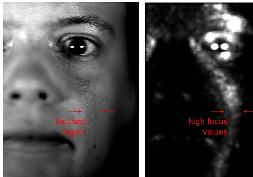
4.5 Optical reconstruction                                                                                  27

Figure 4.5: For each lateral point (x, y), the focus values Fxy (z) are maximized, which delivers the desired
  z-coordinate. Simultaneously, the height information of the face and the corresponding texture are extracted.

a higher dynamic range.

Figure 4.6: The VRML-model combines the surface data left with the precisely fitting texture file middle to
  form the final digital model right.

As the new detector is very light-sensitive, the hologram quality is less critical than it was before. Even
holograms with a very low image contrast may still be used for the reconstruction.

Surface extraction
Next step is to find the object surface. After digitization of the real image, the object is represented as
focussed points in the image volume. Such, the digitized volume is an overlay of focussed and unfocussed
points. Focussed regions carry more information in a higher spectral range than unfocussed regions.
A measure for the degree of focus is given by a mathematical operator measuring image contrast, as
the local contrast in small neighbourhood will be larger for focussed points.
4.5 Optical reconstruction                                                                                       28

Figure 4.7: Example for set of tomograms of the real image at different positions.
  In each slice, some of the areas of the face are sharp, while others are unfocussed.
  The focus progresses from the tip of the nose up to the ears.

  Figure 4.8: Sketch of a local pixel neighbourhood U5 (x, y) of the point (x, y) with the size of 5x5 pixels.

Finding the maximal focus values is necessary in order to extract the surface information of the recorded
object or face. Comparing focus values along the z-axis delivers a z-value for each lateral point.

The extracted surface can be visualised through the height map, which displays the z-values as coded
gray values; low numbers are dark colours (front) and high numbers are light (back). The height
map is a parallel projected surface and gives the position of the highest sharpness in the real image.
The height map is used to extract the brightness information from the image volume. This extracted
image is called the texture image. This grey scale picture can be dyed with one colour, to create a
more realistic appearance. The height map and the texture image are combined into the final digital
computer model.
4.5 Optical reconstruction                                                                                   29

Figure 4.9: a) one slice of a typical scan shows clear focus profile, which is clearly extracted by b) the focus
  value. White corresponds to high contrast values, black to low contrast values.

Surface visualization
The Virtual Reality Modelling Language (VRML) is used to store the 3D-model as a plane text file.
The graphical file format is intended to be a universal exchange format for multimedia and is used in a
variety of applications such as engineering and scientific visualization [OR2]. It can be displayed using
a VRML-plugin, for example the blaxxun contact plugin (http://www.blaxxun.com). It additionally
provides information about illumination, background color and the viewing position.

The actual topometry information is given as a set of three-dimensional points (x,y,z), where the
neighbouring points are connected to form a trigonal model. The texture image is mapped precisely
on the object surface.

In order to add the texture to the polygonal model, the node positions are projected into the texture
image coordinate system. These projected node coordinates are also written in the VRML-file, so that
the texture is positioned correctly in the resulting model.
5 Computed Tomography                                                                                  30

5 Computed Tomography

5.1 Introduction

In order to develop a new technique to do high precision facial soft tissue thickness measurements, it is
necessary to compare the holographic data to bone surface information. Computed Tomography (CT)
can be a good way to provide these data.

We have been familiar with radiographs for about a century now. Anatomy is presented on the analog
film as a continuum with nearly arbitrary fine transitions. The human eye does not recognise any steps
in intensity; only arbitrarily fine gradations of grey levels and continuous transitions for contours are
given.

Computed Tomography was the first widely used radiological imaging modality which exclusively
provided computed digital images instead of the well known directly acquired analog images. It also
offered images of single discrete slices instead of a super-positioned images of complete body sections.

For an understanding of Computed Tomography it may be helpful to view the human body as a finite
number of discrete slices and volume elements. Each single scan aims to determine the composition of
one transverse cross-section. The slice or section can be imagined as composed of discrete cubic volume
elements. The value of each volume element is displayed in one picture element of the digital image
matrix. For volume elements we often use the term ’voxel’, and for picture elements the term ’pixel’.
In principle, a slice image can be generated in arbitrary orientation. For CT, mostly a transverse
plane (x/y-plane) is scanned directly. The z-axis, orientated perpendicular to the scan and image
plane, is thereby aligned along the axis of rotation of the scanning system, parallel to the body’s
longitudinal axis. Sagittal body sections are approximated by y/z -planes, coronal sections by x/z -
planes. A conventional radiograph shows a modulated distribution of radiation intensity and always
offers a superposition image. Each picture element displays the sum of all contributions to attenuation
[CT1].

Image contrast is defined by the difference in intensity of two neighbouring picture elements or regions.
Contrast in radiographs is dominated by structures with high attenuation such as bone and contrast
media, or by differences in object thickness. Soft tissue structures provide low attenuation; even the in-
troduction of improved detector systems or digital data processing will not alter the situation. For slice
5.1 Introduction                                                                                              31

images, contrast is given directly by the attenuation values of neighbouring volume elements. Contrast
is determined by the composition of the tissues, while neighbouring or superimposed structures have
no or only very little influence [CT1, CT2, CT3, CT4].

For survey radiographs, the relative distribution of the X-ray intensity is recorded; for classical ra-
diographs only the grey value pattern is utilised to derive a diagnosis. In CT, in addition to the
intensity I attenuated by the object, the primary intensity I0 has to be measured in CT to calculate
the attenuation value along each ray from the source to detector.

CT measures and computes the spatial distribution of the linear attenuation coefficient u. However,
the physical quantity u is not very descriptive and is strongly dependent on the spectral energy used.
The attenuation coefficient is displayed as a so-called CT value relative to the attenuation of water.
In honour of the inventor of CT, CT values are specified in Hounsfield Units (HU). For a tissue with
attenuation coefficient uT the CT value is defined as
                                              (uT − uwater )
                                 CT value =                  · 1000 HU .                                   (5.1)
                                                 uwater

Figure 5.1: The Hounsfield scale. CT values characterize the linear attenuation coefficient of the tissue in each
  volume element relative to the µ-value of water. The CT values of different tissues are therefore defined to
  be relatively stable and to a high degree independent of the X-ray spectrum.

On this scale, water and each water-equivalent tissue with uT = uwater has the value 0 HU by definition.
Air corresponds to a CT value of −1000 HU. Lung tissue and and fat exhibit negative CT values due
to their lower density and the resulting lower attenuation (ulung < uwater ). Most other body areas
exhibit positive CT values , due to the physical density of muscle and most of the soft tissue. For bone,
the increased density is responsible for a higher attenuation and therefore for higher CT values, up to
2000 HU. CT values of bone are more strongly dependent on X-ray energy than water, and increase
5.2 Segmentation of CT data 32
with reduced high voltage settings, as known in the contrast settings in conventional radiographs.
The Hounsfield scale has no upper limit. For medical scanners a range from −1024 HU up to +3071 HU
is provided. Consequently, 4096 (= 212 ) different values are available (= 4096 grey levels ) [CT1].
Spiral CT means the fast and continuous scanning of complete volumes; it replaces the sequential
scanning of single slices, which means only discrete sampling along the z-axis. The patient is trans-
ported continuously through the tube at a speed of one to two slice collimations per 360◦ rotation. For
multi-slice systems and sub-second rotation times, the table speed can be increased [CT5]. The image
reconstruction in spiral CT is in principle the same as in sequential CT; identical algorithms, convo-
lution kernels and same hardware are used. However, an additional pre-processing step is required,
the so-called z-interpolation. The calculation of images from any 360◦ spiral data segment leads to
artefacts, since different object sections are measured at start and at the end of any such segment. The
resulting artefacts correspond exactly to the motion artefacts known from sequential CT.
5.2 Segmentation of CT data
In many medical-imaging applications, image segmentation plays a crucial role, by automating or
facilitating the delineation of anatomical structures and other regions of interest. The growing size
and number of these medical images have necessitated the use of computers to facilitate processing and
analysis. Image segmentation algorithms play a vital role in numerous medical-imaging applications.
Partial-volume effects are artefacts that occur where multiple tissue types contribute to a single pixel,
resulting in a blurring of intensity across the boundaries. The most common approach to face partial-
volume effects is to produce segmentations that allow regions to overlap, called soft segmentations.
Standard approaches use hard segmentations, a binary decision on whether a pixel is inside or outside
the object.
Figure 5.2: Illustration of partial-volume effects.
Left: ideal image.
Right: acquired image.
Thresholding is a simple and effective way for obtaining a segmentation of images in which different5.2 Segmentation of CT data 33 structures have contrasting intensities. Thresholding does create a binary partitioning of the image intensities. The segmentation is achieved by grouping all pixels with intensities greater than the threshold into one class, and all other pixels into another class.
6 Experiment - probands                                                                              34

6 Experiment - probands

6.1 Introduction

Traditional methods for static object topometry show good results when using a long acquisition time.
Topometry of living persons is much more complex, and when using the traditional methods, artefacts
may occur.

To overcome these shortcomings, holographic topometry was developed to digitize human faces. Li-
ving individuals can be captured without moving artefacts due to the extreme short acquisition time.
Additionally, the pulse energy has to be high enough to illuminate the whole face in a homogeneous
way.

Many aspects of the holographic topometry have been described in previous dissertations. Bongartz
[Ho-In4] described the method for the first time. He implemented speckle illumination and the use of
a mirror setup [Ho-In6]. Frey introduced a direct real image scanning [Ho-In7], and Thelen focussed
on the reconstruction methods and image refinement [Ho-In8]. Finally, Hirsch introduced the digital
holographic topometry by introducing a CCD sensor to record the hologram [Ho-In9].

In the setup for this experiment, we used the first mobile camera for daylight capture. The persons
are captured into a pulsed portrait hologram. The camera is described in chapter 6.3.

After capture, the hologram plate is processed chemically. The reconstruction is done in a different
unit. The real image is digitized slice by slice, to capture the whole 3D information in an image stack.

Finally, the surface is determined numerically from the image volume. The final digital surface model
is visualized as a 3D model (e.g. VRML).

6.2 Set up experiment

For the experiment, we searched for 25 probands with following characteristics:
6.2 Set up experiment                                                                              35

   • age range: between 18-23,

   • Caucasian ethnics,

   • no amalgam fillings,

   • male-female ratio approx 1/1.

Before starting the experiments, we also described the physical morphology of the face, measured the
Body Mass Index of all probands, and we took three photographs of the probands face: one frontal,
one lateral, and one half profile.

                               Figure 6.1: Photographs of the probands’ face.
                          left: frontal, middle: lateral (profile), right: half profile.

We chose a small group of probands within a limited age range. Probands with dental amalgam
fillings were excluded as these fillings provoke a scattering effect on CT (Computed Tomography)
images. This would definitely influence the soft tissue measurements in the cheek area. Additionally,
the dental scattering creates a lot of artefacts on the working model.

Different dental occlusions show different facial shapes e.g. a mandibular protrusion is typical for a
class-III occlusion. In our experiment, all probands showed a class-I occlusion, in order to obtain a
moderate facial outline.

Finally, we included 13 female and 12 male probands in the study. All probands received an ’in-
formed consent’, explaining the aim of the experiment and the recording technique of both holographic
recording and low-dose Computed Tomography.

Probands were explained that they can stop contributing to the experiment at all times. They were
also informed that participating in the experiment included no risk. Women who (thought they) were
6.3 Mobile holographic camera 36 pregnant, giving breast-feeding, or could not show any adequate contraception method, were excluded from the experiment. A face is recognisable from the hologram. Probands were guaranteed that all data were strictly inves- tigated at CAESAR (center of advance European studies and research) in Bonn, and at the University of Düsseldorf. Pictures of proband’s faces and holographic surfaces could only be shown in scientific articles and presentations. Finally, probands received a small contribution fee. Both the low-dose CT and the hologram were taken at the University Hospital Gent, Belgium. For the convenience of the probands, both recordings were performed in one session. 6.3 Mobile holographic camera A new mobile system was designed in cooperation with Geola UAB. The HSF-MINI has a compact design and can be used both on site and in laboratory. The main characteristics of this camera is its flexibility in time and space: the whole set up can be done in a short time, and the system can be transported in a little van. The camera also works in normal light conditions. A shutter is mounted on the mobile camera to make daylight recordings. For comparison, the holographic lab system works at red room light. Figure 6.2: Mobile holographic unit HSF-MINI developed together with Geola Uab (Lithuania). The camera is shown without the diffuser plates for eyes-safe operation. The tower on the right houses (from top to bottom) the control unit, the laser power supply, the amplifier power supply and the cooling unit.
You can also read