Snow water equivalents exclusively from snow depths and their temporal changes: the SNOW model - HESS
←
→
Page content transcription
If your browser does not render page correctly, please read the page content below
Hydrol. Earth Syst. Sci., 25, 1165–1187, 2021
https://doi.org/10.5194/hess-25-1165-2021
© Author(s) 2021. This work is distributed under
the Creative Commons Attribution 4.0 License.

Snow water equivalents exclusively from snow depths
and their temporal changes: the 1SNOW model
Michael Winkler1, , Harald Schellander1,2, , and Stefanie Gruber1
1 ZAMG   – Zentralanstalt für Meteorologie und Geodynamik, Innsbruck, Austria
2 Department of Atmospheric and Cryospheric Sciences, University of Innsbruck, Austria
 These authors contributed equally to this work.

Correspondence: Michael Winkler (michael.winkler@zamg.ac.at) and Harald Schellander (harald.schellander@zamg.ac.at)

Received: 3 April 2020 – Discussion started: 17 April 2020
Revised: 25 January 2021 – Accepted: 25 January 2021 – Published: 5 March 2021

Abstract. Reliable historical manual measurements of snow          new model offers a means to derive robust SWE estimates
depths are available for many years, sometimes decades,            from historical snow depth data and, with some modification,
across the globe, and increasingly snow depth data are also        to generate distributed SWE from remotely sensed estimates
available from automatic stations and remote sensing plat-         of spatial snow depth distribution.
forms. In contrast, records of snow water equivalent (SWE)
are sparse, which is significant as SWE is commonly the
most important snowpack feature for hydrology, climatology,
                                                                   1   Introduction
agriculture, natural hazards, and other fields.
   Existing methods of modeling SWE either rely on de-             Depth (HS) and bulk density (ρb ) are fundamental char-
tailed meteorological forcing being available or are not in-       acteristics of a seasonal snowpack (e.g., Goodison et al.,
tended to simulate individual SWE values, such as seasonal         1981; Fierz et al., 2009). Their product yields the areal den-
“peak SWE”. Here we present a new semiempirical multi-             sity [kg m−2 ] of the snowpack, which is often referred to
layer model, 1SNOW, for simulating SWE and bulk snow               as snow water equivalent (SWE). Water resource manage-
density solely from a regular time series of snow depths. The      ment, agricultural applications, hydrological modeling, cli-
model, which is freely available as an R package, treats snow      mate analyses, natural hazard assessments, and many other
compaction following the rules of Newtonian viscosity, con-        fields depend on good estimates of SWE. The mass of wa-
siders errors in measured snow depth, and treats overburden        ter stored in the snowpacks is often more relevant than
loads due to new snow as additional unsteady compaction; if        snow depth. Particularly seasonal SWE maxima, i.e., peak
snow is melted, the water mass is stepwise distributed from        SWE (SWEpk ), is required for, for example, discharge or
top to bottom in the snowpack. Seven model parameters are          flood forecasting as well as analyses of climate and extremes.
subject to calibration.                                            The latter, in turn, rely on long-term or “historical” data.
   Snow observations of 67 winters from 14 stations, well-         While measurements of HS are relatively widely available,
distributed over different altitudes and climatic regions of the   the more useful value of SWE is more difficult to determine
Alps, are used to find an optimal parameter setting. Data from     and is consequently relatively poorly known, hampering ef-
another 71 independent winters from 15 stations are used for       forts to understand SWE variance and related vast manage-
validation. Results are very promising: median bias and root       ment practices. To address this limitation, this paper focuses
mean square error for SWE are only −3.0 and 30.8 kg m−2 ,          on developing a robust method to derive SWE from more
and +0.3 and 36.3 kg m−2 for peak SWE, respectively. This          readily available and historical records of HS.
is a major advance compared to snow models relying on em-
pirical regressions, and even sophisticated thermodynamic
snow models do not necessarily perform better. As such, the

Published by Copernicus Publications on behalf of the European Geosciences Union.
1166                                                M. Winkler et al.: Snow water equivalents exclusively from snow depths

1.1    Measurements of HS and SWE                                  1.2     Modeling SWE

Measuring HS is relatively easy (e.g., Sturm and Holmgren,         1.2.1    Thermodynamic snow models
1998): manual measurements at a certain point only require
a rod or ruler (e.g., Kinar and Pomeroy, 2015), and decades-       Modern snow models such as Crocus (e.g., Vionnet et al.,
long series of daily HS measurements exist in many regions         2012), SNOWPACK (e.g., Lehning et al., 2002), SNTHERM
– both lowlands and alpine areas (e.g., Haberkorn, 2019).          (Jordan, 1991), or the dual-layer model SNOBAL (Marks
More recently, automatic measurements of HS (mostly sonic          et al., 1998) resolve mass and energy exchanges within the
or laser distance ranging) have become available, typically        ground–snow–atmosphere regime in a detailed way by de-
with sub-hourly resolution (McCreight and Small, 2014), and        picting the layered structure of seasonal snowpacks. Echo-
remotely sensed HS vastly expands on the areal coverage            ing Langlois et al. (2009), these models, which comprise
of manual measurements, although in most cases at the cost         all energy balance and temperature index models, will be
of accuracy, temporal resolution, and regularity. (Dietz et al.    termed “thermodynamic snow models” hereafter. They all
(2012) give a general review of remotely sensed HS measure-        need atmospheric variables as input, primarily precipitation,
ments, and Painter et al. (2016) provide a thorough overview.      temperature, humidity, wind speed, and radiative fluxes, and
Deems et al. (2013) review lidar measurements of HS, while         even simplified variants require temperature and/or precipi-
Garvelmann et al. (2013) and Parajka et al. (2012) illustrate      tation (e.g., De Michele et al., 2013) or climatological means
the potential of time-lapse photography.)                          thereof (Hill et al., 2019). Avanzi et al. (2015) provide a
   In contrast, measurements of SWE (or ρb ) are more dif-         good review. Unfortunately, many valuable long-term HS se-
ficult (e.g., Sturm et al., 2010): manual measurements are         ries do not have accompanying data required to force a ther-
time consuming and require some skill and basic equipment          modynamic snow model for calculating the associated SWE,
like snow tubes or snow sampling cylinders. For most snow-         and parametrizing or downscaling forcing data from other
packs, a pit has to be dug to consider the layered structure       sources in turn is susceptible to errors. Thermodynamic snow
of the snowpack (e.g., Kinar and Pomeroy, 2015). As a con-         models are typically able to simulate snowpack features be-
sequence, SWE measurements are much more sparse than               yond SWE and bulk snow density (e.g., grain types, energy
HS measurements (e.g., Mizukami and Perica, 2008; Sturm            fluxes, stabilities), but they are not applicable to derive SWE
et al., 2010), their accuracy is lower, and time series are        exclusively from HS.
shorter. Only in very rare cases are consecutive, decades-long
measurement series available (e.g., in Switzerland; cf. Jonas      1.2.2    Empirical regression models
et al., 2009). Even for regularly measured “snow courses”,
data are sporadic in time and rarely more than biweekly. Also      Statistical models of SWE derived from HS and a combina-
automatic measurements of SWE are not at all comparable in         tion of date, altitude, and regional parameters (like Guyen-
quality and quantity with automated HS measurements. They          non et al., 2019; Pistocchi, 2016; Gruber, 2014; Mizukami
are quite expensive, often inaccurate, still at a developmen-      and Perica, 2008; Jonas et al., 2009) are hereafter termed
tal stage, and/or suffer from significant problems if not in-      “empirical regression models” (ERMs), and a listing of ex-
tensively maintained throughout the snowy season. Methods          isting approaches is given in Avanzi et al. (2015). ERMs rely
involve weighing techniques (snow scales; e.g., Smith et al.,      on the strong, near-linear dependence between HS and SWE
2017; Johnson et al., 2015), pressure measurements (snow           (cf., e.g., Jonas et al., 2009). According to Gruber (2014)
pillows; e.g., Goodison et al., 1981), upward-looking ground       and Valt et al. (2018), HS describes 81 % and 85 % of SWE
penetrating radar (e.g., Heilig et al., 2009), passive gamma       variance, respectively. This behavior is based on the narrow
radiation (e.g., Smith et al., 2017), cosmic ray neutron sens-     range within which the majority of bulk snow densities lie
ing (e.g., Schattan et al., 2019), and L-band Global Navi-         and leads to the well-known characteristic of HS–SWE–ρb
gation Satellite System signals (e.g., Koch et al., 2019); the     datasets: log-normally distributed HS and SWE and normally
biggest and best serviced network of automated SWE mea-            distributed ρb (e.g., Sturm et al., 2010).
surements most likely is SNOTEL with about 800 sites in               In most ERMs, absolute, single-day HS observations are
western North America (Avanzi et al., 2015).                       the only snow characteristics used. Depending on calibra-
   Remotely sensed SWE data are not operationally available        tion focus, they can usually only adequately model single
for the local and point scale, and deriving this snow property     SWE features (e.g., mean SWE or SWEpk , midwinter or
from satellite products at sub-kilometer resolution is still not   spring). For example, those calibrated for good estimates of
possible (Smyth et al., 2019). Furthermore, the available au-      mean SWE fail to model SWEpk sufficiently well; those de-
tomated measurements and rough estimates of SWE remote             signed for SWEpk often give poor SWE results during phases
sensing instruments are only available for some 20 years at        with shallow snowpacks. Typically, they simulate unrealistic
best (e.g., SNOTEL, operated since the late 1990s), which          mass losses during phases with compaction only by meta-
is short compared to decades-long daily HS data (e.g., Kinar       morphism and deformation. The timing of SWEpk as well as
and Pomeroy, 2015).                                                the duration of high snow loads cannot be modeled well. As

Hydrol. Earth Syst. Sci., 25, 1165–1187, 2021                                       https://doi.org/10.5194/hess-25-1165-2021
M. Winkler et al.: Snow water equivalents exclusively from snow depths                                                                        1167

stated by Jonas et al. (2009), those models cannot be used to     Table 1. Different types of SWE models, categorized by their essen-
“convert time series of HS into SWE at daily resolution or        tial input. TD, SE, and ERMs are abbreviations for thermodynamic,
higher”, because they may “feature an incorrect fine struc-       semiempirical, and empirical regression models, respectively.
ture in the temporal course of SWE”. Therefore, ERMs are
not suitable to calculate SWE for individual days.                          Essential input                    TD       SE       ERMs
   McCreight and Small (2014) not only use single-day HS                    HS (single values)                                      x
values for their regression model but also the “evolution” of               HS (regular records)               xa        x
daily HS. They make use of the negative correlation of HS
                                                                            One or more
and ρb at short timescales and their positive (negative) cor-
                                                                            atmospheric variable(s)            x
relation at longer timescales during accumulation (ablation)
phases. This development is limited by the fact that the model              Date                               xb                   x
parameters can only be estimated through regressions relying                Location parametersc               xb                   x
on “at least three” training datasets of HS and ρb from nearby            a or another precipitation input; b only essential in some cases,
stations. This disqualifies the model of McCreight and Small              e.g., for parameterizations; c altitude, regional climate, etc.
(2014) for assigning SWE to long-term and historical HS se-
ries as consecutive SWE measurements are not available.
                                                                  1.3   Motivation for a new approach
1.2.3   Semiempirical models
                                                                  Table 1 summarizes the classification of SWE models with
An alternative approach that links HS and SWE throughout a        respect to their essential input. Given the strong need for
snowy season without the need of further meteorological in-       robust SWE data for numerous applications and the com-
put is provided by Martinec (1977) and revisited by Martinec      bined simplicity and effectiveness of semiempirical models,
and Rango (1991): they use a method already developed by          it is notable that this type of model has received little atten-
Martinec (1956) “to compute the water equivalent from daily       tion in recent years. Here we focus on developing a robust
total depths of the seasonal snow cover”. Snow compaction is      semiempirical model that can be used to capitalize on more
expressed as a time-dependent power function. Each layer’s        widespread modern-day HS data, as well as to derive SWE
snow density ρn after n days is given by ρn = ρ0 · (n + 1)0.3 ,   from historical HS records.
where ρ0 is the initial density of the snow layer. Martinec and       The semiempirical method of determining SWE presented
Rango (1991) set ρ0 to 100 kg m−3 ; Martinec (1977) varied        here maintains the key feature of previous semiempirical
it from 80 to 120 kg m−3 . This computation is meant to give      models considering only the change of snow depth as a proxy
good results for the seasonal maximum snow water equiva-          for the various processes altering bulk snow density and snow
lent (SWEpk ). It is shown that the older the snow, the less      water equivalent, but it further
important is the correct choice of the crucial parameter ρ0
(Martinec, 1977; Martinec and Rango, 1991). Their model             – bases its (dry) snow densification function on Newto-
interprets “each increase of total snow depth [. . . ] as snow-       nian viscosity;
fall” and if “the total snow depth remains higher than the
                                                                    – provides a way to deal with small discrepancies between
settling by [the power function], this is also interpreted as
                                                                      model and observation (on the order of HS measurement
new snow. If the snow depth drops lower than the value of
                                                                      errors);
the superimposed settling curve of the respective snow lay-
ers, it is interpreted as snowmelt, and a corresponding wa-         – takes into account unsteady compaction of underlying,
ter equivalent is subtracted. In this way the water equivalent        older snow layers due to overburden snow loads; and
of the snow cover can be continuously simulated” (Martinec
and Rango, 1991). Rohrer and Braun (1994) improved this             – densifies snow layers from top to bottom during melting
model particularly for the ablation season by further increas-        phases without automatically modeling mass loss due to
ing density whenever melt conditions are modeled and by in-           runoff.
troducing a maximum possible snow density of 450 kg m−3 .
                                                                     The ideas for the last three advancements are taken from
    Semiempirical snow models simulate individual snowpack
                                                                  Gruber (2014), who described them but did not suitably
layers and make use of simple densification concepts. (Hence
                                                                  include them as a model. The new modeling approach is
they are not “fully” empirical.) They cannot model snow
                                                                  named 1SNOW. Its code is available as niXmass package
properties aside from SWE and density, but their only re-
                                                                  in R (R Core Team, 2019), which also includes other models
quired input is a HS record: no forcing by atmospheric con-
                                                                  that use snow depth and its temporal change (nix. . . Latin for
ditions is needed. In some respects these models bridge the
                                                                  snow) to simulate SWE (i.e., snow mass).
gap between thermodynamic models and ERMs.

https://doi.org/10.5194/hess-25-1165-2021                                        Hydrol. Earth Syst. Sci., 25, 1165–1187, 2021
1168                                                       M. Winkler et al.: Snow water equivalents exclusively from snow depths

Figure 1. Schematic of 1SNOW.

Table 2. Summary of compaction processes and processes forcing mass changes that are integrated in 1SNOW, as well as processes that are
ignored.

           Module                   Process
           New Snow                 significant rise of HS and enhanced compaction due to overburden load (Overburden submodule)
           Dry Compaction           significant decline of HS due to dry metamorphism∗ and/or deformation∗
           Drenching                significant decline of HS due to wet metamorphism∗ and runoff through melt (Runoff submodule)
           Scaling                  adjustments to small changes of HS within threshold deviation τ
           Ignored                  snow drift compaction∗ and mass changes due to the following:
                                    rain on snow, runoff during snowfalls, wind drift, small snowfalls, sublimation, and deposition
         ∗ Terminology follows Jordan et al. (2010).

2     Method                                                                 HS := HSobs . Analogously, the layer’s snow water equiva-
                                                                             lent equals total snow water equivalent: swe = SWE := ρ0 ·
Snow compacts over time due to various processes. Jordan                     HSobs , with new-snow density ρ0 being an important param-
et al. (2010) categorize them in snow drift, dry and wet                     eter of the 1SNOW model (cf. Sect. 3). The treatment of the
metamorphism, and deformation. The 1SNOW model cannot                        first snow event is illustrated at t = 2 in Fig. 1.
deal with snow drift; however, it differentiates between the
other processes. Table 2 shows the processes modeled and                     2.2    Dry Compaction module
their corresponding 1SNOW modules and outlines the pro-
cesses that are ignored. The specific modules are described                  Martinec and Rango (1991) used a power function to de-
in Sect. 2.2 and 2.3, and a schematic of the model is shown                  scribe densification of aging snow, because this way errors in
in Fig. 1.                                                                   initial density ρ0 become less relevant over time. As 1SNOW
                                                                             also aims to robustly model SWE of ephemeral snowpacks
2.1    Preliminary: the first snow layer                                     (e.g., at low-elevation sites) and as overburden load is con-
                                                                             sidered in a particular way (Sect. 2.3.1), it is not expedient to
For nonzero snow depth observations (HSobs > 0) after a                      have a direct dependence between density and age of a layer.
snow-free period, the following features are assigned to the                 Instead of a power law, 1SNOW (like most modern snow
1SNOW model snowpack. There is one snow layer (ly = 1).                      models) simulates snow compaction by way of Newtonian
Thickness of this model layer (hs) and total model snow                      viscosity with associated exponential densification over time
depth (HS) are equal and set to observed snow depth: hs =                    (e.g., Jordan et al., 2010). In the Dry Compaction module, the

Hydrol. Earth Syst. Sci., 25, 1165–1187, 2021                                                   https://doi.org/10.5194/hess-25-1165-2021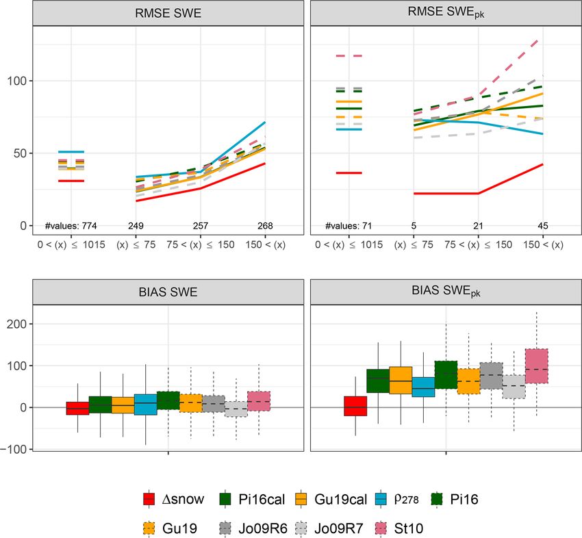
M. Winkler et al.: Snow water equivalents exclusively from snow depths                                                           1169

densifying effects of dry metamorphism and deformation are             core module as its output determines the subsequent process
combined, by adopting the relations of Sturm and Holmgren              decisions and which module will be applied.
(1998) and De Michele et al. (2013):
                                                                       2.3     Process decisions
hs(i, t − 1)           σ (i, t)
                       b
             =1 + 1t ·          ,                                      At every point in time, after the Dry Compaction module
  hs(i, t)             η(i, t)
                                                                       is run, observed HSobs (t) and modeled HS(t) are compared.
                                      ly(t)
                                      X                                The 1SNOW’s process decision algorithm confronts the dif-
                with b
                     σ (i, t) = g ·            swe(î, t)
                                                                       ference 1HS(t) = HSobs (t) − HS(t) with τ [m]. τ is another
                                          î=i                         tuning parameter of 1SNOW (see Sect. 2.4). Technically, τ is
                                            k·ρ(i,t)
                and η(i, t) = η0 · e                   .        (1)    a threshold deviation and defines a limit of 1HS(t) whose
                                                                       overshooting, adherence, and undershooting heads for one of
   t and t − 1 are the points in time of the actual and the pre-       the modules described in the following Sect. 2.3.1 to 2.3.3.
ceding snow depth observation, respectively. The time span             Table 2 links them to snow physics.
between these measurements is 1t, which is in general ar-
bitrary, but usually it is taken to be 1 d. hs(i, t) is the actual     2.3.1    New-Snow module
modeled thickness of the ith snowP layer. The actual depth of
the total snowpack is HS(t) = hs(i, t).                                In the case of 1HS(t) > +τ , meaning observed snow depth
                                      i                                is significantly higher than modeled snow depth, a new-snow
   The individual snow water equivalents of the layers are             event is assumed to have occurred, and a new top snow layer
given by swe(i, t), and their
                         P sum represents total mass of                is modeled (see at t = 2 and t = 7 in Fig. 1). Other mod-
the snowpack SWE(t) = swe(i, t). The vertical stress at                els have implemented this mechanism (e.g., Martinec and
                              i                                        Rango, 1991; Sturm et al., 2010). However, 1SNOW goes
the bottom of layer i is given by b σ (i, t) (De Michele et al.,
                                                                       further and explicitly models the effect of overburden load
2013). It is induced by the sum of loads overlying layer i,
                                                                       on underlying layers, defined as their enhanced densification
with ly(t) being the total number of snow layers.
                                                                       due to stress, which is applied by the weight of new snow.
   The Newtonian viscosity of snow η is made density-
                                                                       Grain bonds get broken; grains slide, partially melt, and warp
dependent in the framework of the 1SNOW model (follow-
                                                                       (Jordan et al., 2010); and the layers densify comparatively
ing Kojima, 1967), but dependencies on temperature or grain
                                                                       rapidly and strongly. 1SNOW interprets overburden load as
characteristics are consciously ignored – due to the lack of
                                                                       an “unsteady and discontinuous” stress on the snowpack, un-
information on it when dealing with pure snow depth data.
                                                                       der which snow presumably does not react as a viscous New-
The actual density of layer i is ρ(i, t); it equals swe(i,t)
                                                     hs(i,t) ; k and   tonian fluid. As long as the time between two consecutive
η0 are tuning parameters of the Dry Compaction module (see
                                                                       observations, 1t, is on the order of at least some hours, dis-
Sect. 3).
                                                                       continuity is an intrinsic feature of the process.
   To avoid excessive compaction, a crucial parameter is in-
                                                                          The New Snow module realizes the effect of overburden
troduced in 1SNOW, as was done by Rohrer and Braun
                                                                       load through the Overburden submodule by reducing each
(1994): ρmax . It defines the maximal possible density of a
                                                                       layer’s thickness, hs(i, t), using the dimensionless “overbur-
snow layer and, consequently, also the maximum bulk snow
                                                                       den strain”, (i, t), defined as
density. Finding its optimal value for 1SNOW is subject to
calibration (Sect. 2.4).                                                                               ρ(i,t)
                                                                                               −kov ρmax
   According to Eq. (1), the rate of densification of a cer-           (i, t) =cov · σ0 · e             −ρ(i,t)

tain snow layer is linearly dependent on the overlying snow                      with σ0 = 1HS(t) · ρ0 · g.                        (2)
load bσ (i, t) and exponentially dependent on the layer’s den-
sity ρ(i, t). Sturm and Holmgren (1998) conclude that this                cov [Pa−1 ] is another tuning parameter of the model (see
difference is one reason why “snow load plays a more limited           Sect. 2.4) and controls the importance of the unsteady com-
role in determining the compaction behavior than grain and             paction due to overburden load. According to Sturm and
bond characteristics and temperature”. Equation (1) links the          Holmgren (1998) (and in consistency with Eq. 1) snow load
densification rate to the layer age (but indirectly by the use         has a linear effect on the bulk density. Therefore, (i, t) is a
of density) and not directly as it was the case with the power-        linear function depending on the load, applied by the over-
law approach by Martinec and Rango (1991). Consequently,               lying new snow on the underlying layers. This load is well
1SNOW’s compaction is not directly dependent on layer age,             approximated by σ0 [Pa]; the larger the overburden load,
which is a prerequisite for the functioning of the Overburden          the stronger the compaction. (The overburden load does not
submodule (Sect. 2.3.1).                                               fully equal σ0 , since 1HS(t) is not the depth of the new
   The Dry Compaction module is illustrated by the light blue          snow, but it is the difference between modeled depth “be-
arrows in Fig. 1. This module is applied at every point in             fore” knowing about the new-snow event and observed depth
time (except if there is no snow; see t = 1 in Fig. 1). It is the      “after” the new-snow event. An iterative calculation would

https://doi.org/10.5194/hess-25-1165-2021                                            Hydrol. Earth Syst. Sci., 25, 1165–1187, 2021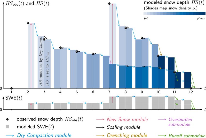
1170                                                 M. Winkler et al.: Snow water equivalents exclusively from snow depths

be more precise; however, Eq. (2) proved to be an adequate              η0∗ (i, t) is then used instead of η0 in Eq. (1) to re-
compromise between simplicity and accuracy.) In order to             calculate the compaction of individual layers. HS(t) now
avoid (i, t) > 1, cov is restricted at least to the range of val-   equals HSobs (t). In most cases all layers get slightly more
ues between 0 and the minimum value of the data record for           or slightly less compacted by the Scaling module than by the
 1                                           1
σ0 . As σ0 hardly ever exceeds 1000 Pa, σ0 normally is larger        Dry Compaction module. Only at rare occasions the scaling
            −3
than 1 × 10 Pa−1 . This value marks an upper bound for cov           does not lead to a compaction but to a small stretching of the
(Sect. 2.4). Dimensionless kov controls the role of a certain        snowpack. This only happens if there was a small increase
snow layer’s density on (i, t) and has to be specified by cali-     in observed snow depth and very little modeled dry meta-
bration (see Sect. 2.4). The density dependence of (i, t) was       morphic compaction; the condition HS(t) + τ > HSobs (t) >
chosen to be exponential and is constrained by ρmax .                HSobs (t − 1) has to be fulfilled. Of course, such stretching
   The “overburden strain” (i, t) theoretically lies between 0      does not occur in reality, but also in the model it occurs only
and 1 and compresses all snow layers of the model in the             rarely and at small scale: in any case the stretching is smaller
case of a new-snow event. Practically, (i, t) is often close to     than τ . The issue is accepted as a model artifact, not least
zero (in this study 90 % of all computed  values are smaller        because the stretching enables the very valuable adjustment
than 0.09) and extremely rarely higher than 0.3 (in this study       to HSobs at every point in time without forcing mass gains for
only 9 out of 10 000).                                               insignificant HS raises within the measurement accuracy.
   The intermediate snow layer thicknesses               ∗              In the case when the density of an individual layer ex-
                                 ∗       P ∗ are hs (i, t) =         ceeds ρmax by the scaling process, the excess mass is dis-
(1 − (i, t)) · hs(i, t) and HS (t) = hs (i, t). The com-
                                         i                           tributed layerwise from top to bottom. SWE remains constant
pressed layer’s masses, swe(i, t), remain unaffected during          during scaling, unless it would be necessary to compact all
this process. A new-snow event, identified by the condition          layers beyond ρmax . In this case, the appropriate excess mass
1HS(t) > +τ , of course not only impacts the older snow              is taken from the model snowpack and interpreted as runoff,
and compacts it more strongly but also adds a new-snow               SWE is reduced and all layer thicknesses are cut accordingly
layer and mass to the snowpack (pink arrow at t = 2 and              (see Runoff submodule in Sect. 2.3.3 for details). As τ turns
t = 7 in Fig. 1). The following attributes are given to the          out to be reasonably chosen on the order of a few centime-
new layer: hs(ly, t) = HSobs (t) − HS∗ (t) and swe(ly, t) =          ters by calibration (Sect. 3), the resulting reduction of SWE
hs(ly, t) · ρ0 , and the total snow water equivalent arises:         within the Scaling module is always quite small: for example,
SWE(i, t) = SWE(i, t −1)+swe(ly, t). The model snowpack              with τ = 2 cm and maximum density chosen as 450 kg m−3
with its new properties is subsequently compacted according          (like Rohrer and Braun, 1994), the mass loss due to runoff is
to Eq. (1), and the process decision starts again as described       only 9 kg m−2 .
in Sect. 2.3. The Overburden submodule is illustrated with a            The Scaling module is illustrated as black arrows in Fig. 1.
purple arrow at t = 7 in Fig. 1.                                     Note that the scaling is nothing physical but also nothing sub-
                                                                     stantial in terms of SWE, yet it is a way to utilize the advan-
2.3.2   Scaling module                                               tage of having a measured snow depth at every point in time.
Equations (1) and (2) are highly simplified representations
                                                                     2.3.3   Drenching module
of the complex viscoelastic behavior of snow, and available
HS observations typically only show an accuracy of a few
                                                                     The Drenching module simulates compaction due to liquid
centimeters. The 1SNOW model accepts these inherent in-
                                                                     water percolating from top to bottom through the snowpack,
accuracies by not applying too strict criteria in the process
                                                                     loosening grain bonds and leading to densification (wet snow
decisions described in Sect. 2.3. The threshold deviation τ
                                                                     metamorphism). In the case when observed snow depth at a
acts as a buffer to avoid too frequent gain or loss of mass:
                                                                     certain point in time is significantly lower than modeled snow
in the case of |1HS| ≤ |τ |, the snowpack does not lose mass
                                                                     depth (1HS(t) < −τ ), the Drenching module is activated.
nor gain mass, but mass is kept constant. In order to bene-
                                                                        1SNOW ignores rain on snow since it concentrates on
fit from having a new measurement at every point in time,
                                                                     modeling SWE for pure snow depth records without having
HS(t) is intentionally set to HSobs (t) by the Scaling module.
                                                                     any further information on, for example, precipitation, tem-
   The Scaling module forces a partial revaluation of the pre-
                                                                     perature, and snowfall level. Possibilities of how rain could
vious compaction, which was modeled by the Dry Com-
                                                                     be addressed in future developments are outlined in Sect. 4.6.
paction module between t −1 and t. The best-fitted parameter
                                                                        To cope with the model–observation discrepancy
setting for η0 is temporarily rejected and substituted by η0∗ .
                                                                     1HS(t) < −τ , the Drenching module densifies the model
It would be straightforward to use one adjusted η0∗ (t) for all
                                                                     layers until ρmax is reached, starting from the uppermost
layers. However, this leads to multiple solutions for η0∗ (t),
                                                                     one. Figuratively spoken, a certain layer gets drenched
making it necessary to calculate different η0∗ (i, t) for each
                                                                     until saturation and meltwater is further distributed to the
layer i. See Appendix B for details on that.
                                                                     underlying layer. This process is repeated until transient HS∗
                                                                     equals HSobs (t). One or more layers might reach ρmax .

Hydrol. Earth Syst. Sci., 25, 1165–1187, 2021                                         https://doi.org/10.5194/hess-25-1165-2021
M. Winkler et al.: Snow water equivalents exclusively from snow depths                                                                                               1171

Table 3. The seven parameters of 1SNOW. The last column depicts model sensitivity to changes in the density parameters. The respective
gradients [kg m−2 per kg m−3 ] are means over the whole calibration ranges.

              Parameter        Unit               Optimal        Calibration         Literature                                           Sensitivity
                                                                                                                                             δSWEpk
                                                      value              range       range                                                 δρ0 or δρmax

              ρ0               kg m−3                     81          50–200         75a , 10–350 (70–110)b                               +0.37 (+0.50∗ )
              ρmax             kg m−3                   401          300–600         450c , 217–598d , 400–800e                           +0.24
              η0               106 Pa s                 8.5              1–20        8.5a , 6f , 7.62237g                                 not calc.
              k                m3 kg−1                0.030          0.01–0.2        0.011–0.08a , 0.185h , 0.023f,g , 0.021i             not calc.
              τ                cm                        2.4             1–20        –                                                    not calc.
              cov              10−4 Pa−1                 5.1             0–10        –                                                    not calc.
              kov              –                       0.38           0.01–10        –                                                    not calc.
            a Sturm and Holmgren (1998), b Helfricht et al. (2018) with range for means in brackets, c Rohrer and Braun (1994), d Sturm et al. (2010),
            e Cuffey and Paterson (2010), f Jordan et al. (2010), g Vionnet et al. (2012), h Keeler (1969), i Jordan (1991). See Sect. 2.4 for more details. ∗ The
            value in brackets is the gradient taken from the smaller window between 70 and 90 kg m−3 (cf. Sect. 4.1).

In the case when 1HS(t) is so negative that all model                                     gists consider the density at which snow transitions to firn
snow layers are compacted and densified to ρmax but still                                 to span 400 to 800 kg m−3 (e.g., Cuffey and Paterson, 2010).
HS∗ > HSobs (t), the Runoff submodule is activated, and                                   Still, manual density measurements of seasonal snow used in
runoff R(t) is defined as R(t) = (HS∗ − HSobs (t)) · ρmax .                               previous studies hardly ever exceed 500 kg m−3 (e.g., Jonas
   All layer thicknesses are cut by a respective portion:                                 et al., 2009; Guyennon et al., 2019). Armstrong and Brun
                hs ∗                                                                      (2010) limit it to approximately 400 to 500 kg m−3 too. In
(HS∗ −HSobs )· HSi∗ . This mechanism does not reduce the total
number of layers, but layers potentially get very thin. During                            order to find the best value for ρmax used in 1SNOW, it was
the melt season, where most of the runoff is produced, the                                varied from 300 to 600 kg m−3 .
Runoff submodule is more or less continuously active until                                   Equation (1) needs η0 , the “viscosity at [which] ρ equals
HSobs (t) = 0 and all the snow has been converted to runoff.                              zero” (Sturm and Holmgren, 1998). It is found to be on
For a distinct snowpack from the first snowfall (t1 ) until get-                          the order of 8.5 × 10⁶ Pa s (Sturm and Holmgren, 1998),
                                   t2
                                   P                                                      6 × 10⁶ Pa s (Jordan et al., 2010), and 7.62237 × 10⁶ Pa s
ting snow-free again (t2 ), one has R(t) = SWEpk .                                        (Vionnet et al., 2012). During the calibration process for the
                                             t1
   In Fig. 1 the Drenching module is shown by the brown                                   1SNOW model, η0 was varied from 1 to 20×106 Pa s. Param-
arrows and its Runoff submodule by the green arrows.                                      eter k, the second necessary parameter in Eq. (1), was varied
                                                                                          from 0.011 to 0.08 m3 kg−1 by Sturm and Holmgren (1998)
                                                                                          depending on climate region and respective different types of
2.4   Calibration                                                                         snow. However, they cite Keeler (1969) in their Table 2 with
                                                                                          values for k for “Alpine-new” snow of up to 0.185 m3 kg−1 .
1SNOW has seven parameters that have to be calibrated: ρ0 ,                               In more complex snow models k is set to 0.023 m3 kg−1
ρmax , η0 , k, τ , cov , and kov (cf. Table 3). For the first four                        (see Crocus: bη in Eq. (7) by Vionnet et al. (2012); and
parameters, one finds suggestions and ranges in the literature:                           also in Eq. (2.11) of Jordan et al., 2010) or 0.021 m3 kg−1
   Sturm and Holmgren (1998) do not address the critical-                                 (see SNTHERM: Eq. (29) in Jordan, 1991). Its range for the
ity for the choice of new-snow density; however, they use                                 1SNOW model calibration was set from 0.01 to 0.2 m3 kg−1 .
constant ρ0 = 75 kg m−3 . It is a well-known characteristic                                  There are no references for the latter three parameters.
of new snow to show large variations in densities. Helfricht                              Threshold deviation τ , as mentioned, might be interpreted
et al. (2018) reviewed many studies and give a general range                              as a measure of observation error, is regarded to be on the or-
of 10–350 kg m−3 , narrowing it down to “mean values” be-                                 der of a few centimeters, and was modified from 1 to 20 cm
tween 70–110 kg m−3 . Note that this is daily densities. Sub-                             for calibration. The last two parameters, cov and kov , deter-
daily means of new-snow densities are lower. Helfricht et al.                             mine the role of overburden strain and are newly introduced
(2018), for example, come up with an average of 68 kg m−3                                 in the 1SNOW model. At least the limits of cov could be de-
for hourly time intervals. During the calibration process for                             fined (Sect. 2.3.1) as cov ∈ [0, min( σ10 )]; kov is only known
the 1SNOW model, ρ0 was varied from 50 to 200 kg m−3 .                                    to be a dimensionless, real, positive number. For calibrat-
   The second density-related calibration parameter is ρmax ,                             ing 1SNOW, cov and kov were restrained by [0, 10−3 Pa−1 ]
which is the maximum possible density within the model                                    and [0.01, 10], respectively.
framework. Rohrer and Braun (1994) set such a maximum                                        The calibration performed in this study is based on 1t =
at 450 kg m−3 . Sturm et al. (2010) defined it for five different                         1 d, but longer as well as shorter 1t values are conceivable
climate classes, ranging from 217 to 598 kg m−3 . Glaciolo-

https://doi.org/10.5194/hess-25-1165-2021                                                                    Hydrol. Earth Syst. Sci., 25, 1165–1187, 2021
1172 M. Winkler et al.: Snow water equivalents exclusively from snow depths
and could be handled by the 1SNOW model too. Note, how- In order to ensure an unperturbed validation, the observa-
ever, that at least some calibration parameters will change tion datasets from Austria and Switzerland (1529 SWE–HS
significantly when changing 1t. This gets obvious when pairs) were split into two almost equally big halves: one for
considering new-snow density ρ0 , which of course is differ- model calibration (SWEcal ) and one for validation (SWEval ).
ent if defined for 1 h or for a 3 d time step. The usage of this The two data sources (Gruber, 2014; Marty, 2017) do not ad-
publication’s calibration parameters can, therefore, only be dress the accuracy of the manual SWE observations. Mostly,
suggested for daily snow depth records. SWE measurements made with snow sampling cylinders are
used as references in comparison studies, without address-
2.4.1 Calibration data and method ing their accuracy (e.g., Sturm et al., 2010; Dixon and Boon,
2012; Kinar and Pomeroy, 2015; Leppänen et al., 2018).
The calibration process needs SWE data, which are quite rare López-Moreno et al. (2020) provide a reported range of 3 %–
per se (see Sect. 1), and regular snow depth records from the 13 % and condense the results of their own experiments to an
same places. There are surprisingly few places where both error range of 10 %–15 % for bulk snow density. The ma-
parameters have been consequently observed side by side for jority of SWEcal and SWEval comes from the Hydrographic
many years, e.g., daily HS measurements accompanied by Service of Tyrol, Austria, where snow sampling cylinders
weekly, biweekly, or monthly SWE measurements. (500 cm3 ) are used (Sect. 2.4.1). The repeatability of this
Gruber (2014) collected 14 years of weekly SWE data kind of measurement is estimated at ±4 % for glacier mass
from six stations in the Eastern Alps, measured by the balance studies (Rainer Prinz, University of Innsbruck, Aus-
observers of the Hydrographic Service of Tyrol (Austria) tria, personal communication, 2020). Roughly interpreting
between winters 1998/99 and 2011/12. The measurements these density measurement “variabilities” as relative obser-
of snow depth and water equivalent were made manu- vation errors for SWE, the results for absolute accuracy
ally in snow pits with rulers and snow sampling cylinders would typically spread across the wide range of about 2 to
(500 cm3 ), respectively. The sites range from 590 to 1650 m 50 kg m−2 .
altitude and are situated in relatively dry, inner-alpine regions Model calibration was performed with the statistical soft-
as well as in the Northern Alps and Southern Alps, which ware R (R Core Team, 2019) and the R package optimx
are more humid due to orographic enhancement of precipita- (Nash, 2014). Results were obtained with optimization meth-
tion (see Gruber, 2014, for details). The sites in the Southern ods L-BFGS-B (Byrd et al., 1995) followed by bobyqa (Pow-
Alps even show a moderate maritime influence due to their ell, 2009), which both are able to handle lower and upper
vicinity to the Mediterranean Sea, which is the most impor- bound constraints. The function to be minimized was the root
tant source of moisture for this region (e.g., Seibert et al., mean square error (RMSE) of SWEs from the 1SNOW model
2007). These 6 × 14 = 84 winter seasons cover 1166 mea- and observed SWEs, using the calibration dataset SWEcal .
sured HS–SWE pairs. Besides these SWE measurements,
manual H S measurements are available for every day at the
respective stations. Figure A1 and Table A1 provide a map
3 Results
and a list, respectively.
The second source for SWE measurements used for cali-
This section evaluates the ability of 1SNOW to calculate
bration is Marty (2017). The Swiss SLF (Institute for Snow
snow water equivalents exclusively from snow depths, as
and Avalanche Research) freely provides biweekly SWE and
well as its practicability. Table 3 gives an overview of all pa-
daily HS data from 11 stations in Switzerland. The HS mea-
rameters and summarizes the optimal setting for 1SNOW. A
surements, accompanying the biweekly SWE measurements,
discussion of the best-fitted values and of the model sensitiv-
were compared with the contemporary value of the daily
ity to parameter changes can be found in Sect. 4.
HS records. Only those sites and years where and when the
The minimal RMSE between all SWE observations used
respective values of the daily HS record match the values of
for calibration (SWEcal ) and the respective modeled val-
the biweekly measurements were used for calibration. If this
ues were reached for new-snow density ρ0 = 81 kg m−3 ,
condition is fulfilled, it is supposed that SWE and HS mea-
maximum density ρmax = 401 kg m−3 , viscosity parameters
surements fit together sufficiently well, although they unfor-
η0 = 8.5 × 10⁶ Pa s and k = 0.030 m3 kg−1 , threshold devi-
tunately cannot always be taken exactly at the same place,
ation τ = 2.4 cm, and overburden parameters cov = 5.1 ×
which introduces uncertainty (e.g., López-Moreno et al.,
10−4 Pa−1 and kov = 0.38.
2020). Consequently, nine stations were used, most of them
in the Northern Alps, some inner-alpine, spanning an altitude 3.1 Validation and comparison to other models
range from 1200 to 1780 m, with all in all 56 winters and
363 pairs of HS and SWE measurements. Details are given In this study no quantitative comparison with thermodynamic
in Fig. A1 and Table A1. Other stations and years suffer from snow models was performed, since they need further meteo-
discrepancies caused by too far spatial distances between the rological data and the focus was on data records constrained
measurements and so on. to snow depths. However, the 1SNOW model was thoroughly
Hydrol. Earth Syst. Sci., 25, 1165–1187, 2021 https://doi.org/10.5194/hess-25-1165-2021M. Winkler et al.: Snow water equivalents exclusively from snow depths 1173 Figure 2. Root mean square errors (RMSE) and biases (BIAS) between the 1SNOW model and different empirical regression models from the SWEval observations. The 1SNOW model, models by Pistocchi (2016) and Guyennon et al. (2019), and the “constant density approach” were calibrated with SWEcal data (1SNOW, Pi16cal, Gu19cal, ρ278 ; upper panels, solid lines). Dashed lines indicate the Pistocchi (2016), the Guyennon et al. (2019), the Jonas et al. (2009), and the Sturm et al. (2010) models with their standard parameters (Pi16, Gu19, Jo09R6, Jo09R7, and St10). Jo09R6 and Jo09R7 together illustrate the maximum possible spread of the Jonas et al. (2009) model since Region 6 (R6) and Region 7 (R7) are characterized by the highest and lowest “region-specific offset”, respectively. The upper left panel shows RMSEs for all SWEval values (short horizontal lines) as well as for three SWE classes: SWE ≤ 75, SWE > 150, and intermediate. Analogously for SWEpk (upper right panel), RMSEs are shown. The boxes for the biases (lower panels) encompass 774 values (left panel, SWE) and 71 values (right panel, SWEpk ) and spread from the 25 % to the 75 % quantiles; the whiskers indicate 1.5 times the interquartile range. Units are kg m−2 . evaluated against ERMs. Figure 2 and Table 4 show the re- for Jonas et al. (2009) it was distinguished between regions sults. Even though ERMs do not need meteorological data, (see the caption of Fig. 2). Other contemporary approaches it is not straightforward to calibrate them for new sites and had to be ignored, mostly because of the problematic trans- applications. From the vast number of ERMs (cf. Avanzi ferability of regional parameters (e.g., McCreight and Small, et al., 2015), the ones of Pistocchi (2016) and Guyennon et al. 2014, or Mizukami and Perica, 2008). (2019) were chosen to be fitted to SWEcal . These models are The bias of modeled SWE (lower left panel in Fig. 2) quite new and easy to calibrate. Additionally, an approach is quite low and tends to be positive, meaning SWE is of- simply using a constant bulk snow density at every point in ten slightly overestimated by the ERMs. 1SNOW slightly time was calibrated to fit this study’s data. Thus, 278 kg m−3 underestimates SWE on average, with a median bias of turned out to be the optimal value minimizing root mean −3.0 kg m−2 . The overall good results for the ERMs is not square errors of all SWEcal values. Moreover, Jonas et al. surprising, since they are dedicated to perform well on av- (2009) and Sturm et al. (2010) were used for comparison. erage. The specially calibrated versions of Pistocchi (2016) Unfortunately, calibration of these powerful models would and Guyennon et al. (2019) show a significantly smaller bias have needed much more data than the 780 SWE–HS pairs of than their originals. The model of Jonas et al. (2009) has the SWEcal dataset. Therefore, Jonas et al. (2009) and Sturm the smallest bias for their “Region 7”, encompassing the dry, et al. (2010) were used with their standard parameters, but inner-alpine Engadin as well as parts of the Southern Alps https://doi.org/10.5194/hess-25-1165-2021 Hydrol. Earth Syst. Sci., 25, 1165–1187, 2021
1174                                                            M. Winkler et al.: Snow water equivalents exclusively from snow depths

Table 4. Overview on SWE accuracies of different models and studies. The numbers in brackets represent the results for the example
portrayed in Figs. 3 and 4 from station Kössen in 2008/09. Units are kg m−2 , TD is short for thermodynamic snow models. For model
abbreviations, see caption of Fig. 2.

                Source                            Model                      SWE            SWE        SWE           SWEpk       SWEpk
                                                  (version)                  BIAS          RMSE        MAE            BIAS        RMSE
                This study                        1SNOW                       −3.0      30.8 (21)       21.9        0.3 (-3)        36.3
                                                  Gu19cal                      4.8      39.1 (43)       27.6      63.0 (93)         85.6
                                                  Pi16cal                      5.6      39.4 (47)       28.1     70.3 (106)         80.8
                                                  Jo09R7                      −3.2      39.4 (41)       27.3      52.0 (74)         70.2
                                                  St10                        14.0      45.1 (57)       32.6     91.1 (154)        117.2
                                                  ρ278                        10.6      50.9 (51)       36.3      45.2 (77)         66.4
                Guyennon et al. (2019)            Gu19                                                 49.2
                                                  Pi16cal                                              50.6
                                                  Jo09cal                                              48.5
                                                  St10cal                                              51.0
                Jonas et al. (2009)               Jo09                                 50.9–53.2
                Sturm et al. (2010)               St10 (“alpine”)          29 ± 57
                Vionnet et al. (2012)             Crocus                    −17.3             39.7
                Langlois et al. (2009)            Crocus              −7.9 to −5.4     10.8–12.5
                                                  SNTHERM                 9 to 18.1    18.3–19.3
                                                  SNOWPACK             −0.1 to 5.6      7.4–14.5
                Egli et al. (2009)                SNOWPACK                                      56
                Wever et al. (2015)               SNOWPACK                                ca. 39.5
                Sandells et al. (2012)            SNOBAL                                    30–49                                17–44a
                Essery et al. (2013)              various TDb                               23–77
              a This is not RMSE of SWE but RMSE “from establishment of snowpack to SWE ”. b See Table 10 in Essery et al. (2013): RMSE for
                                       pk                                              pk
              up to 1700 uncalibrated and calibrated simulations.

and the very east of Switzerland (Samnaun), which is partly                     shown in Fig. 2 and Table 4). ERMs tend to model SWEpk
influenced by orographic precipitation from northwesterly                       some days too early, because the date of modeled SWEpk is
flows. In terms of heterogeneity in precipitation climate, “Re-                 shifted towards the date of highest HS (cf. Fig. 4).
gion 7” is comparable to the region where the SWE data of                          Another satisfactory validation result for 1SNOW is shown
this study come from.                                                           in the upper panels of Fig. 2. RMSEs for all SWE values are
   The other three indicators illustrated in Fig. 2 and summa-                  constantly lower than if modeled with ERMs: an RMSE of
rized in Table 4 show the improved performance of 1SNOW                         30.8 kg m−2 (1SNOW) contrasts RMSEs between 39.1 and
compared to ERMs: the latter are intrinsically tied to snow                     50.9 kg m−2 (ERMs). Calibrating the models of Pistocchi
depth (see Sect. 1.2) and are systematically forced to overes-                  (2016) and Guyennon et al. (2019) results in some improve-
timate SWEpk . Note that the maximal SWE of a winter sea-                       ment; at least they perform much better than the “constant
son does not necessarily equal the highest measured SWE,                        density approach” after the calibration. The model of Jonas
because measurements are only taken weekly or biweekly.                         et al. (2009) does a decent job even without recalibration.
In the vast majority of the SWE records used for this study,                    The method by Sturm et al. (2010) is calibrated with data
the highest seasonal observation is followed by at least one                    from the Rocky Mountains. For this comparison, the “alpine”
lower SWE reading. Sometimes real SWE might be higher                           parameters of Sturm et al. (2010) were taken; however, con-
after the highest measurement of a winter season was taken,                     ditions might differ too much from the European Alps. Abso-
but a thorough data check revealed that this is of minor im-                    lute errors in SWE increase with increasing SWE. For snow-
portance here. It is sufficiently precise to assume that mea-                   packs lighter than 75 kg m−2 , 1SNOW’s RMSE is 17 kg m−2 ,
sured seasonal maximum SWE equals SWEpk ; 1SNOW’s                               between 75 and 150 kg m−2 it is 26 kg m−2 , and for snow-
bias of SWEpk is very minor, only +0.3 kg m−2 . Moreover,                       packs heavier than 150 kg m−2 it increases to 43 kg m−2 .
the 1SNOW model works better for the timing of SWEpk (not

Hydrol. Earth Syst. Sci., 25, 1165–1187, 2021                                                        https://doi.org/10.5194/hess-25-1165-2021
M. Winkler et al.: Snow water equivalents exclusively from snow depths 1175
The 1SNOW model also has a small RMSE of 36.3 kg m−2
when modeling SWEpk (Fig. 2, upper right; Table 4, last two
columns). Also the SWEpk RMSEs for the different SWE
classes are very close to those for SWE, which emphasizes
1SNOW’s ability to model all individual SWEs comparably
well. The evaluated ERMs have much higher, mostly at least
doubled, errors in simulated SWEpk . Remarkably, the sim-
ple ρ278 approach performs relatively well. In the case when
the Jonas et al. (2009) model is suitably adjusted to regional
specialties, it performs better than the other ERMs but still
significantly worse than 1SNOW.
These results demonstrate that 1SNOW outperforms
ERMs. This can be argued on the basis of Fig. 2 but even
more when looking at the ERM studies themselves: Jonas
et al. (2009) provide RMSEs between 50.9 and 53.2 kg m−2
for their standard model, which are quite high values com-
pared to the findings of the study in hand (39.4 kg m−2
for their Region 7; see Table 4). One explanation could
be that Jonas et al. (2009) as well as other ERM studies
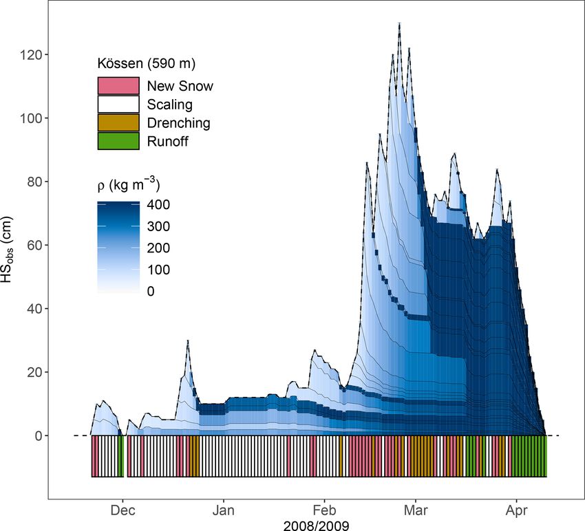
rely on a huge amount of (but still diverse measurements in Figure 3. Winter of 2008/09 in Kössen (Northern Alps, Austria)
terms of record length) observations per season. The 1SNOW portrays density evolution as simulated by the 1SNOW model. Re-
model study only consists of data from selected stations with spective (sub)modules are depicted in colors at the bottom, when-
ever activated. Note that 1SNOW is not intended to simulate indi-
long and regular SWE readings, where also ERMs seem to
vidual layers but to calculate daily SWE, SWEpk , and daily bulk
work better. Guyennon et al. (2019) summarize their and
density. Descriptions and discussions of some features are given in
other studies’ validation results using MAE, the mean ab- the text.
solute error. Sturm et al. (2010) assess the bias for their
“alpine” model at +29 kg m−2 with a standard deviation of
57 kg m−2 , and they outline that “in a test against exten-
sive Canadian data, 90 % of the computed SWE values fell
within ±80 kg m−2 of measured values”. Table 4 provides
an overview and shows that ERMs generally perform better
with this study’s data than with their original data.
3.2 Illustration
Figure 1 schematically shows the functioning of the 1SNOW
model. A practical example is provided in Fig. 3, based
on the optimal calibration parameters found during this
study. Kössen, the station shown, is situated in the North-
ern Alps at 590 m (cf. Fig. A1). Although it is a low-lying
place, it is known to be snowy, which is, firstly, due to
intense orographic enhancement of precipitation associated
with northwesterly to northeasterly flows in the respective
region (Wastl, 2008) and, secondly, comparably frequent in-
flow of cold continental air masses from northeast. Showing
the example of Kössen should emphasize the versatile us- Figure 4. SWE simulations and observations (SWEobs ) for the win-
ability of 1SNOW: it is not only designed for high areas with ter 2008/09 in Kössen (cf. Fig. 3). Details and abbreviations are
deep, long-lasting snowpacks but also for valleys with shal- given in the text (Sect. 3.2) and summarized in Fig. 2.
low, ephemeral snowpacks. Winter 2008/09 was chosen be-
cause 1SNOW shows a rather typical performance in terms of
RMSE and BIAS in Kössen (see Table 4, values in brackets), tifies 2 d with snowfall (purple markings) and models two
and because some important, model-intrinsic features can be respective snow layers, which can be distinguished by the
addressed and discussed: thin black line in Fig. 3. After about a week, the snowpack
Late November 2008 brought the first, however transient, starts to melt, the snow layers reach ρmax very fast (the blue
snowpack of the season (Fig. 3). The 1SNOW model iden- shading gets dark), and finally all the snow was converted
https://doi.org/10.5194/hess-25-1165-2021 Hydrol. Earth Syst. Sci., 25, 1165–1187, 20211176 M. Winkler et al.: Snow water equivalents exclusively from snow depths
to runoff (green markings). In the second half of Decem- 4 Discussion and outlook
ber, there were 3 d with new snow, followed by a strong
decline in snow depth. In the frame of the 1SNOW model, Model results clearly depend on the parameters. Their opti-
this HS decrease is only possible if the layers “get wet” mal values are subject to calibration. The choice of the best-
and the Drenching module is activated (marked in brown). fitted values is rated and discussed in the following Sect. 4.1
The layers get denser, starting at the top. However, the de- to 4.5. Section 4.6 to 4.8 cover possible future developments,
crease was “manageable” only by increasing the two upper- accuracy issues, and 1SNOW’s applicability in remote sens-
most layer densities to ρmax and making the third layer just ing.
a bit denser. Not all layers got to ρmax , and no runoff was
modeled. The 1SNOW model conserves the two dense lay- 4.1 New-snow density ρ0
ers until the end of the winter, which can clearly be seen
in Fig. 3. One could interpret the layers as consisting of Being aware of both the potentially large variations of new-
melt forms or a refrozen crust. However, such interpreta- snow density and the possible cruciality of this parameter for
tions require caution, because modeling detailed layer fea- SWE simulation by the 1SNOW model, ρ0 was chosen to be
tures is not the intention of 1SNOW. During January Fig. 3 a constant in the framework of the model. ρ0 = 81 kg m−3
shows a phase where modeled values and observations agree turned out to be the best choice after calibration with SWEcal .
to a high extent, and only the Scaling module is activated This value clearly lies within the broader frame of possible
for small adjustments (white markings). Small “stretching new-snow densities (Table 3) and quite closely to 75 kg m−3
events” can be recognized, e.g., on 2 and 3 January, where by Sturm and Holmgren (1998), but it is found in the lower
model snow layers are set less dense in order to avoid too fre- part for typical new-snow densities (e.g., Helfricht et al.,
quent mass gains. During continuous snowfalls in February 2018). A possible explanation is that the SWE measurement
the successive darkening of the blue layer shadings illustrates records used for the calibration tend to underrepresent late
a phase of consequent compaction, which actually lasts until winter and spring conditions. Regular (weekly, biweekly)
March, when strong decreases in HSobs start to activate the observations capture the short melt seasons worse than the
Drenching module. Still, runoff is not yet produced. Only in longer accumulation phases. Therefore, SWE records might
the second half of March does the whole model snowpack be biased towards early and midwinter new-snow densities,
reach ρmax (“saturation”). The ablation phase is clearly dis- which are lower (e.g., Jonas et al., 2009). Still, there are also
tinguishable and lets the snowpack vanish rapidly towards some indications that using, for example, 100 kg m−3 as con-
10 April 2009. stant for new-snow density when modeling SWE results in an
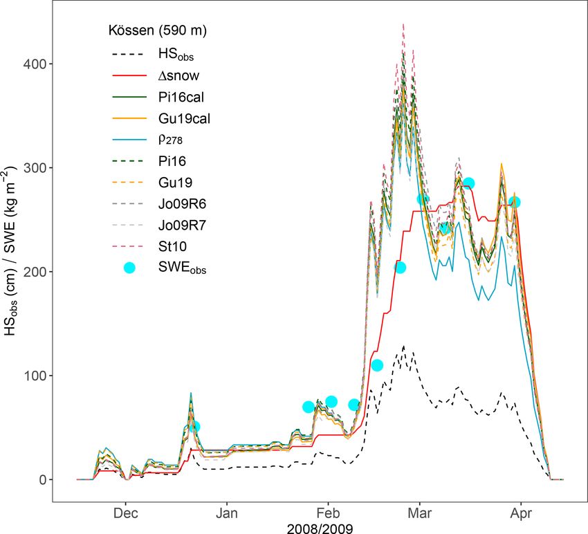
The snow depth record of Kössen from 2008/09 was also overestimation of precipitation (up to 30 % according to Mair
used to compare different ERMs and 1SNOW to SWE ob- et al., 2016). The calibrated value for ρ0 can be regarded as
servations (Fig. 4). These measurements (light blue circles) a reasonable result, even more when only considering it as a
are part of the SWEval sample and were manually made model parameter but not as a physical constant.
with snow sampling cylinders; one after the December 2008 The sensitivity analysis illustrated in Fig. 5 confirms the
snowfall and another nine on a nearly weekly basis between importance of a good choice of ρ0 . Increasing ρ0 leads
late January and late March 2009. Figure 4 also provides to a decrease of the relative bias of seasonal SWE max-
various model results, and some respective key values are ima (SWEpk ). Note the definition of the relative bias in the
given in Table 4. Not surprisingly and thus evidently, the caption of Fig. 5. In absolute values, too small ρ0 values
ERM SWE curves follow the snow depth curve (black dashed cause too small SWEpk values, while using higher values
line). The first four measurements are not well simulated leads to an overestimation of SWEpk . This behavior supports
by the 1SNOW model (red line); the ERMs perform bet- the above-mentioned tendency to overestimate precipitation
ter in this illustrative case. But after the stronger snowfalls when choosing constant 100 kg m−3 as new-snow density. As
of February the picture changes indisputably in favor of the expected, the new-snow density is the most crucial parameter
1SNOW model. This is a typical pattern, because ERMs of the 1SNOW model (cf. Table 3). The median relative bias
are too strongly tied to snow depth and therefore mostly of SWEpk changes by −0.46 % per +1 kg m−3 if the whole
(1) overestimate SWEpk , (2) model its occurrence too early, calibration range of ρ0 is considered to calculate the sensitiv-
and (3) – most importantly – force modeled SWE to reduce ity (50–200 kg m−3 ). This means a median change in SWEpk
during pure compaction phases after snowfalls. Evidently, of +0.37 kg m−2 when ρ0 is risen by +1 kg m−3 . If the lim-
the ability of 1SNOW to conserve mass during the phases its are restricted more tightly around the optimal value, the
with dry metamorphism is its strongest point, not only in gradient is even steeper: −0.62 % and +0.50 kg m−2 per
Kössen 2008/09 but also on average (cf. Fig. 2 and Table 4). +1 kg m−3 , respectively, when the gradient is approximated
for the range 70–90 kg m−3 . The widely used ρ0 value of
100 kg m−3 , consequently, causes a median overestimation
of SWEpk of about 12 % in the 1SNOW model. Daily SWE
shows the same behavior (not shown), and users should be
Hydrol. Earth Syst. Sci., 25, 1165–1187, 2021 https://doi.org/10.5194/hess-25-1165-2021You can also read