Characterising spatio-temporal variability in seasonal snow cover at a regional scale from MODIS data: the Clutha Catchment, New Zealand ...
←
→
Page content transcription
If your browser does not render page correctly, please read the page content below
Hydrol. Earth Syst. Sci., 23, 3189–3217, 2019
https://doi.org/10.5194/hess-23-3189-2019
© Author(s) 2019. This work is distributed under
the Creative Commons Attribution 4.0 License.

Characterising spatio-temporal variability in seasonal
snow cover at a regional scale from MODIS data:
the Clutha Catchment, New Zealand
Todd A. N. Redpath1,2 , Pascal Sirguey1 , and Nicolas J. Cullen2
1 National   School of Surveying, University of Otago, P.O. Box 56, Dunedin, New Zealand
2 Department    of Geography, University of Otago, P.O. Box 56, Dunedin, New Zealand

Correspondence: Todd A. N. Redpath (todd.redpath@otago.ac.nz)

Received: 17 January 2019 – Discussion started: 25 January 2019
Revised: 18 June 2019 – Accepted: 19 June 2019 – Published: 2 August 2019

Abstract. A 16-year series of daily snow-covered area             cover conditions being out of phase across the catchment.
(SCA) for 2000–2016 is derived from MODIS imagery to              Furthermore, it is demonstrated that the sensitivity of SCD to
produce a regional-scale snow cover climatology for New           temperature and precipitation variability varies significantly
Zealand’s largest catchment, the Clutha Catchment. Filling        across the catchment. While two large-scale climate modes,
a geographic gap in observations of seasonal snow, this           the SOI and SAM, fail to explain observed variability, spe-
record provides a basis for understanding spatio-temporal         cific spatial modes of SCD are favoured by anomalous air-
variability in seasonal snow cover and, combined with cli-        flow from the NE, E and SE. These findings illustrate the
matic data, provides insight into controls on variability. Sea-   complexity of atmospheric controls on SCD within the catch-
sonal snow cover metrics including daily SCA, mean snow           ment and support the need to incorporate atmospheric pro-
cover duration (SCD), annual SCD anomaly and daily snow-          cesses that govern variability of the energy balance, as well
line elevation (SLE) were derived and assessed for tempo-         as the re-distribution of snow by wind in order to improve the
ral trends. Modes of spatial variability were characterised,      modelling of future changes in seasonal snow.
whilst also preserving temporal signals by applying raster
principal component analysis (rPCA) to maps of annual SCD
anomaly. Sensitivity of SCD to temperature and precipitation
variability was assessed in a semi-distributed way for moun-      1   Introduction
tain ranges across the catchment. The influence of anoma-
lous winter air flow, as characterised by HYSPLIT back-           Globally, seasonal snow packs represent an important, yet
trajectories, on SCD variability was also assessed. On av-        vulnerable water resource (Barnett et al., 2005; Mankin
erage, SCA peaks in late June, at around 30 % of the catch-       and Diffenbaugh, 2015) and play a major role in earth–
ment area, with 10 % of the catchment area sustaining snow        atmosphere energy exchange (Estilow et al., 2015). A decline
cover for > 120 d yr−1 . A persistent mid-winter reduction        in seasonal snow-covered area (e.g. Estilow et al., 2015; Bor-
in SCA, prior to a second peak in August, is attributed to        man et al., 2018) and shifts in the timing of snowmelt runoff
the prevalence of winter blocking highs in the New Zealand        have been observed in many regions of the world (e.g. Mc-
region. In contrast to other regions globally, no significant     Cabe and Clark, 2005; Lundquist et al., 2009; Klein et al.,
decrease in SCD was observed, but substantial spatial and         2016). While most observations of reduced seasonal snow-
temporal variability was present. rPCA identified six distinct    covered area come from the Northern Hemisphere (Bor-
modes of spatial variability, characterising 77 % of the ob-      man et al., 2018), negative trends have been observed over
served variability in SCD. This analysis of SCD anomalies         short timescales for both the alpine region of Australia (Bor-
revealed strong spatio-temporal variability beyond that asso-     mann et al., 2012) and much of the South American Andes
ciated with topographic controls, which can result in snow        (Saavedra et al., 2018). Despite the relatively recent estab-

Published by Copernicus Publications on behalf of the European Geosciences Union.
3190                                                         T. A. N. Redpath et al.: Clutha Catchment snow cover variability

lishment of the Snow and Ice Network (SIN) of alpine au-             coarse spatial resolution in the case of passive microwave
tomatic weather stations (Hendrikx and Harper, 2013), long-          sensors, and/or complications associated with complex ter-
term records of snow occurrence and persistence are rare in          rain (Lemmetyinen et al., 2018). Despite the progress in map-
New Zealand (Fitzharris et al., 1999). This scarcity of data         ping SCA, reliable determination of snow depth, particularly
has limited the empirical characterisation of seasonal snow          in complex terrain, remains challenging. Modern, very high
processes. Subsequently, little is known about the persis-           resolution stereo-capable imagers show promise for retriev-
tence of seasonal snow across large areas of the Southern            ing snow depth over large areas, from space, although the
Alps / Kā Tiritiri o te Moana, the variability associated with      influence of topography on uncertainties and complications
snow persistence from year to year, and the climatic influ-          introduced by shadows in alpine terrain demand attention
ences on such variability. Previous work to assess historical        (Marti et al., 2016).
trends in snow water equivalent (SWE) in the main hydro-                Although direct observation of SWE from space re-
electric catchments of the South Island of New Zealand,              mains complicated, methodologies for extracting SCA from
which was largely model driven, revealed substantial tem-            MODIS imagery can now provide relatively long records of
poral variability, but no long-term trend from the 1930s to          spatio-temporal variability in SCA, itself a useful climatic in-
the 1990s (Fitzharris and Garr, 1995). Conversely, modelling         dicator (Clark et al., 2009; Estilow et al., 2015). This is evi-
work undertaken to assess future impacts of climate change           denced by the recent emergence of studies examining spatial
on seasonal snow in New Zealand predicts a substantial re-           and temporal variability in seasonal snow cover, and snow
duction overall in seasonal snow cover duration (SCD), the           cover climatologies, across medium to large spatial scales
snow proportion of precipitation and peak snow accumula-             (e.g. Gascoin et al., 2015; Saavedra et al., 2017, 2018).
tion through the 21st Century (Hendrikx et al., 2012; Jobst             This paper aims to achieve the following:
et al., 2018).
   The apparent absence of any long-term trend in seasonal               1. produce a snow cover climatology for the Clutha Catch-
snow in New Zealand (Fitzharris and Garr, 1995) and the                     ment, New Zealand, for the years 2000–2016 – the snow
associated uncertainty resulting from a scarcity of observa-                cover climatology is defined here as the characterisa-
tional data provides clear motivation for the construction of               tion of the expansion and depletion of the seasonal snow
an updated observational record of seasonal snow in New                     cover over the course of an average hydrological year;
Zealand’s Southern Alps. The need to understand likely fu-               2. leverage the snow cover climatology to examine basin-
ture scenarios of seasonal snow cover underscores the impor-                wide temporal variability in snow-covered area and
tance of such data. Remote sensing offers a means to mitigate               snowline elevation and assess whether any negative
the limitations imposed by a scarcity of in situ observations               trend is detectable over the study period;
of seasonal snow, albeit over a relatively limited time span.
   Remote sensing has provided substantial advances in the               3. characterise spatial modes of temporal variability in
quantification of seasonal snow variability, with imaging sen-              snow cover duration in order to better understand spatio-
sors supporting spatial and temporal resolutions that allow a               temporal variability across the catchment;
range of scales to be explored. Space-borne satellite imagers,
particularly optical sensors, provide a synoptic view and have           4. assess the sensitivity of variability of SCD to variability
provided a step change in capability for mapping and char-                  in temperature, precipitation and synoptic-scale climate
acterising snow-covered areas, although trade-offs exist be-                processes.
tween competing resolutions (Andersen, 1982; Dozier, 1989;
                                                                     This is achieved by leveraging MODIS imagery to produce
Nolin and Dozier, 1993; Hall et al., 2002, 2015; Rittger et al.,
                                                                     a 16-year time series of daily snow-covered area. While the
2013; Sirguey et al., 2009). For example, the MODerate res-
                                                                     mapping of snow-covered area from MODIS imagery is a
olution Imaging Spectroradiometer (MODIS), operating on
                                                                     mature approach (Hall et al., 2002; Sirguey et al., 2009;
board TERRA since 2000, and on AQUA since 2002, per-
                                                                     Dozier et al., 2009; Nolin, 2010; Rittger et al., 2013), char-
mits near-daily mapping of snow-covered area (SCA) at con-
                                                                     acterising the spatial and temporal variability observed in the
tinental to global spatial scales, despite relatively coarse spa-
                                                                     MODIS time series requires the application of robust geospa-
tial resolution. The advance of geostationary meteorological
                                                                     tial and statistical techniques. Here, specifically the appli-
satellites such as Himawari 8 and 9 sees comparable spa-
                                                                     cation of spatialised principal component analysis (PCA) is
tial resolution to MODIS acquired in near real time (Bessho
                                                                     central to the efficient characterisation of spatio-temporal
et al., 2016). Multi-spectral sensors such as Sentinel-2A and
                                                                     variability.
B and Landsat 8 continue to improve the temporal resolution
of imagery suitable for mapping snow at resolutions of 10–
30 m (Malenovský et al., 2012; Roy et al., 2014). Passive and        2    The Clutha Catchment
active microwave sensors offer the capacity to retrieve esti-
mates of snow water equivalent directly from space-borne             With a mean annual discharge of ∼ 530 m3 s−1 (Murray,
platforms but also suffer substantial limitations, including         1975), the Clutha River drains New Zealand’s largest catch-

Hydrol. Earth Syst. Sci., 23, 3189–3217, 2019                                        www.hydrol-earth-syst-sci.net/23/3189/2019/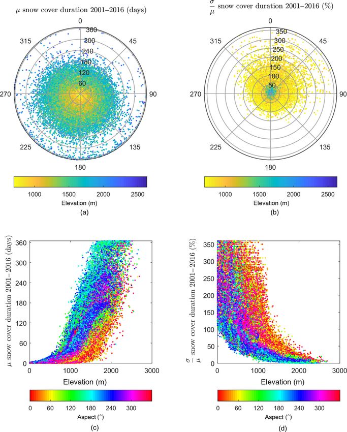
T. A. N. Redpath et al.: Clutha Catchment snow cover variability                                                           3191

ment with an area of approximately 20 800 km2 (area nor-         tention. While modelling studies indicate that significant fu-
malised flow ∼ 800 mm yr−1 ). It is a watershed of primary       ture changes in the snow hydrology of the Clutha Catchment
importance to the both the Otago Region and New Zealand as       are likely (e.g. Poyck et al., 2011; Jobst, 2017; Jobst et al.,
a whole. Addressing the rapidly growing water needs within       2018), observational studies of snow hydrology have been
the Clutha Catchment presents a future challenge as demands      discontinuous and mostly limited to small sub-catchments
for urban water supply and irrigation for agriculture and hor-   (e.g. Fitzharris et al., 1980; Fitzharris and Grimmond, 1982;
ticulture increase, alongside long-standing hydro-electricity    Sims and Orwin, 2011).
commitments. Originating on the Main Divide of the South-           Seasonal snow underpins winter tourism, further con-
ern Alps (maximum elevation of ∼ 2800 m), much of the            tributing to the local economy (Hopkins, 2014). There are
headwater flows are derived from rainfall and the melt of        four commercial downhill ski areas, as well as a cross-
alpine snow cover, along with minor contributions from           country ski area, clustered in the Queenstown–Wanaka area.
glaciers (76 km2 , or 0.04 %, of the catchment is glacierised;   All ski areas have undergone expansion works in recent
Brunk and Sirguey, 2018). Annual precipitation totals may        years, with further expansion planned. A substantial heli-ski
exceed 4000 mm on the western margin of the catchment and        industry is also based out of Queenstown and Wanaka. The
can be less than 400 mm in inland basins. There is no strong     commercial ski season typically runs from mid-June to early
seasonality in precipitation. The contribution of snowmelt to    October; however, opening dates and season length are vari-
the annual streamflow of the Clutha River is estimated to be     able, with lifts not operating until mid-July in the “winter of
10 % by the time it reaches the Pacific Ocean (Kerr, 2013);      discontent” of 2011 (Hopkins, 2015). Whilst modelling work
however, this proportion is substantially higher for alpine      suggests that the duration of natural snow packs for ski areas
sub-catchments and large inland basins, where it may ex-         in Otago will be substantially reduced, and snowmaking will
ceed 30 %–50 %. Importantly, the spatio-temporal variability     become increasingly important with future climate change
in seasonal snow within the catchment is currently not well      (Hendrikx and Hreinsson, 2012), industry participants per-
understood. Some large tributaries arise in the semi-arid in-    ceive inter-annual variability as having a greater impact on
land basins of Central Otago, where annual precipitation may     ski seasons (Hopkins, 2014, 2015).
be as low as 400 mm yr−1 , an order of magnitude less than          Within the catchment, forest cover at elevations above
on the Main Divide (Macara, 2015). The Clutha Catchment          1000 m is limited. According to version 4.1 of the New
includes the Dart, Rees, Shotover, Kawarau, Matukituki,          Zealand Land Cover Database (Landcare Research, 2015),
Wilkin, Hunter, Nevis and Manuherikia rivers. Further refer-     forest constitutes 2.84 % of the total area of 6602 km2 above
ences to specific catchments within this paper will be made      1000 m (Table S1 in the Supplement). Given the difficul-
to the Upper Clutha (Clutha up-stream of Cromwell, includ-       ties associated with recovering reliable SCA estimates from
ing lakes Wanaka and Hawea), Kawarau (west of Cromwell,          MODIS in forested areas (Raleigh et al., 2013), the low pro-
including Lake Wakatipu), Lower Clutha (downstream of            portion of forest land cover is advantageous for the applica-
Cromwell) and the Manuherikia Basin, north-east of Alexan-       tion of remote sensing techniques compared to many other
dra (Fig. 1).                                                    mid-latitude locations.
   Water demands within the catchment are driven by hydro-
electric power generation, and irrigation. The Clutha River
hosts two nationally significant hydro-electric power stations
at the Clyde (432 MW) and Roxburgh (320 MW) dams, and            3     Data and method
smaller hydro-electric power stations operate on tributaries.
Irrigation is particularly important in the central and east-    3.1    MODIS multispectral imagery and MODImLab
ern basins of the catchment, where climate is characterised
by much lower rainfall than the mountainous regions near         MODIS is a useful sensor for mapping snow-covered area
the Main Divide of the Southern Alps, or the coastal lower       (Barnes et al., 1998; Hall et al., 2002; Sirguey et al., 2009;
reaches of the Clutha (Murray, 1975; Hinchey et al., 1981;       Painter et al., 2009; Rittger et al., 2013). In terms of spec-
Macara, 2015). An important aspect of irrigation schemes in      tral resolution, the SWIR bands 6 (1640 nm) and 7 (2130 nm)
drought-prone basins such as the Manuherikia is the capture      permit the implementation of the normalised difference snow
and storage of runoff generated by spring snowmelt for use       index (NDSI) and also facilitate enhanced discrimination of
later in summer (Hinchey et al., 1981). Two major local ir-      snow from other targets when spectral unmixing is utilised
rigation dams, the Falls Dam in the upper Manuherikia and        (Sirguey et al., 2009). Additionally, global daily to near-daily
the Fraser Dam west of Alexandra, have estimated snowmelt        re-visit times allow temporally dynamic phenomena to be
contributions of 15 % and 20 % respectively (Kerr, 2013).        captured, while also maximising the likelihood of cloud-free
Despite a long history of hydrological research and manage-      retrievals. Furthermore, the spatial resolution is useful for
ment, the role of snow within the catchment and the impact       monitoring change at regional scales whereby image fusion
of variability in the extent and duration of winter snow cover   techniques can be employed to map snow using the 250 m
in the Central Otago mountain ranges have received little at-    resolution of MODIS bands 1 and 2, offering an improve-

www.hydrol-earth-syst-sci.net/23/3189/2019/                                   Hydrol. Earth Syst. Sci., 23, 3189–3217, 2019

3192                                                        T. A. N. Redpath et al.: Clutha Catchment snow cover variability

Figure 1. Context map of the Clutha Catchment, including snowmelt contribution to streamflow for rivers of stream order 4 and greater,
and snowmelt contribution data from Kerr (2013). The boundaries of the Upper Clutha, Kawarau and Manuherikia sub-catchments are also
included. Elevation and relief data from Columbus et al. (2011); lake outlines and geographic place names are sourced from the LINZ
Topographic Database and stream network and catchment boundaries from MfE River Environments Classification (Snelder et al., 2010).

ment over the native 500 m resolution of MODIS bands 3–7             for snow mapping from MODIS imagery, found that overall
(e.g. Sirguey et al., 2008).                                         MODImLab compared well with several alternatives when
   Gascoin et al. (2015) highlighted the suitability of              applied in the European Alps, Pyrenees and Moroccan Atlas
MODIS-derived snow cover products for characterising tem-            Mountains.
poral variability in SCA and providing insight into regional            MODImLab employs a spectral unmixing approach (in
snow climatology for the Pyrenees Mountains. Among sev-              contrast to NDSI correlation applied elsewhere) to MODIS
eral robust methodologies for mapping SCA from MODIS                 images which have undergone preprocessing, including
imagery (Masson et al., 2018), MODImLab (Sirguey et al.,             wavelet-based image fusion to facilitate mapping of snow
2009) is used here due to its desirable capabilities and             at 250 m resolution (Sirguey et al., 2008), and a rigorous
specific performance in the Southern Alps. Snow cover                atmospheric and topographic correction, ATOPCOR (Sir-
mapping using MODImLab for the Waitaki Catchment in                  guey et al., 2009, 2016; Sirguey, 2009; Masson et al., 2018).
New Zealand (immediately north of the Clutha Catchment)              In accounting for terrain-reflected irradiance and mitigat-
achieved a mean absolute error (MAE) < 10 % when com-                ing shadow, the topographic correction of MODImLab im-
pared with higher-resolution (15 m) ASTER reference prod-            proves the performance of snow mapping in rugged alpine
ucts (Sirguey et al., 2009). Masson et al. (2018), while not-        terrain (Sirguey et al., 2009; Sirguey, 2009), typical of New
ing the difficulty of balancing high recall and high precision       Zealand’s Southern Alps. MODImLab operates on the basis

Hydrol. Earth Syst. Sci., 23, 3189–3217, 2019                                      www.hydrol-earth-syst-sci.net/23/3189/2019/
T. A. N. Redpath et al.: Clutha Catchment snow cover variability                                                            3193

of eight possible end-members (three being snow and one          small regions of the Main Divide (Fig. 4). Implementation
of ice), originally characterised in the New Zealand context.    of the cloud-filling algorithm provided temporally continu-
The pasture, rock and debris end-members are expected to         ous maps of daily fSCA. For convenience, the time series
align well with the land cover classes detectable within the     was processed into 365 d blocks, corresponding to the New
Clutha Catchment at the MODIS scale (i.e. > 250 m) (Ta-          Zealand hydrological year (HY, 1 April–31 March). These
ble S1). Re-projection of tiles from the MODIS L1B swath         annual gap-filled time series provide the basis for further
is handled by the swath-to-grid module within MODImLab.          analysis of snow cover climatology and variability.
Imagery was resampled to a 250 m grid, in New Zealand
Transverse Mercator (NZTM) projection.                           3.3     SCD and derived metrics

3.2     Snow-covered area time series                            The snow cover climatology can be considered initially in
                                                                 terms of the SCD for each hydrological year, that is, the num-
The central process underlying this study was the con-           ber of days on which snow lies on the ground. SCD can be
struction of a continuous time series of daily, virtually        considered hypsometrically per discrete elevation bands (e.g.
cloud-free, fractional snow-covered area (fSCA) maps for         Gascoin et al., 2015), or spatially per pixel, as it is presented
the Clutha Catchment from MODIS imagery. Collection              here. Spatial determination allows SCD to be mapped across
6 (C6) MODIS/TERRA L1B swath granules were down-                 the catchment. SCD was calculated as the number of days
loaded for all available observations from 1 April 2000 to       for which a pixel exceeded a minimum fSCA to avoid skew-
31 March 2016. Re-projection, preprocessing and mapping          ing the time series by spurious short-lived snowfall events
of fSCA was carried out using MODImLab (see full descrip-        and heavy frost detected as snow cover. In this case, the min-
tion in Sirguey et al., 2009), before implementing a cloud-      imum threshold fSCA (fSCAt ) was set to 50 %, consistent
filling algorithm to build the final 16-year daily cloud-free    with the approach of Sirguey et al. (2009).
fSCA data cube used for subsequent derivation of metrics            Calculating the SCD for each hydrological year from 2001
and analysis (Fig. 2). In this case, the data cube is a four-    to 2016 (which represents the winter of the previous calen-
dimensional data space with two geographic dimensions (i.e.      dar year) also allowed the calculation and mapping of the
easting and northing), a temporal dimension and the fSCA         mean (µSCD ) and standard deviation (σSCD ) of SCD across
dimension.                                                       the catchment, over the 16-year period. In order to charac-
                                                                 terise and map associated variability, the coefficient of varia-
3.2.1    Cloud detection and gap filling                         tion (CVSCD ) was also calculated as follows:
                                                                             σSCD
The presence of cloud, and mis-classification of cloud, or       CVSCD =          .                                           (1)
                                                                             µSCD
cloud shadows, as snow pixels is a common problem in mul-
tispectral remote sensing (Dozier et al., 2008). The develop-    The (CVSCD ) provides an efficient means to calculate the rel-
ment of a robust snow cover climatology benefits from hav-       ative dispersion of data about the mean (Brown, 1998) and
ing a cloud-free daily time series. This was achieved through    has been used in other studies of spatio-temporal variability
the implementation of the time trajectory interpolation pro-     in snow cover (e.g. Hammond et al., 2018).
posed by Dozier et al. (2008). The MOD35 cloud cover prod-
uct (Frey et al., 2008) provided the basis for determining the   3.3.1    Basin snow-covered area
cloud-obscured pixels for which fSCA had to be interpo-
                                                                 The temporal variability of snow-covered area across the
lated. Initially, those pixels flagged as “certain cloud” were
                                                                 basin (basin snow-covered area, bSCA) was assessed using
masked. Sparse commission errors, often occurring at the
                                                                 several metrics (Table 1). These bSCA metrics were calcu-
edge of snow cover due to confusion between the spectral
                                                                 lated as the number of days for which snow-covered pixels
signature of cloud and mixed ground and snow pixels, were
                                                                 (fSCA ≥ fSCAt ) comprised at least 10 %, 15 % and 20 % of
mitigated by a morphological erosion of the binary mask
                                                                 the total catchment area. Area thresholds of 10 %, 15 % and
(Haralick et al., 1987). Two dilatations were then applied to
                                                                 20 % were chosen based on basin hypsometry and informed
restore the main cloud structures and conservatively extend
                                                                 by the mean snow-covered area. For each hydrological year,
the edges of cloudy regions. Each daily map of fSCA was
                                                                 the total number of days meeting each bSCA threshold was
combined with the associated daily cloud mask, with cloud
                                                                 calculated. Linear regression was applied to the annualised
affected pixels subsequently flagged for filling by fSCA in-
                                                                 time series for each metric and each threshold to test the pres-
terpolation.
                                                                 ence of any significant temporal trends.
   Gaps resulting from cloudy pixels are then filled as pro-
posed by Dozier et al. (2008), by applying a smoothing spline
interpolant to each pixel–time trajectory. The average dura-
tion of gaps to be filled was < 5 d overall, while areas of
extended maximum cloud duration (> 20 d) were limited to

www.hydrol-earth-syst-sci.net/23/3189/2019/                                    Hydrol. Earth Syst. Sci., 23, 3189–3217, 2019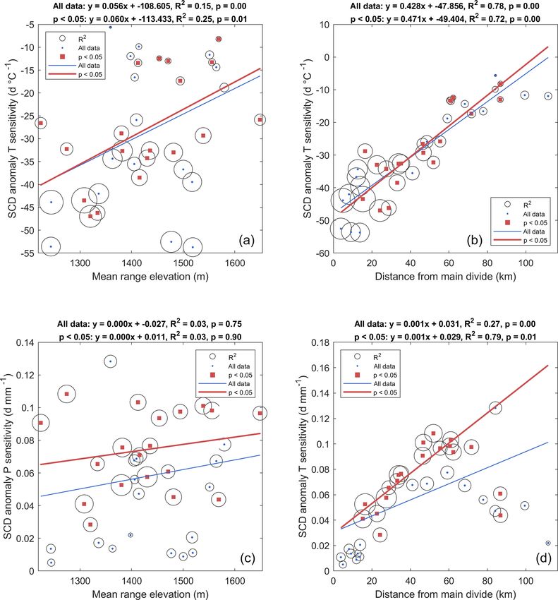
3194                                                          T. A. N. Redpath et al.: Clutha Catchment snow cover variability

Figure 2. MODIS imagery processing chain and subsequent processing (“lightning bolt” symbols) and analytical steps applied. The fractional
snow-covered area (fSCA) data cube facilitates the determination of daily snowline elevation (SLE) and snow-covered area (SCA). The mean
snow cover duration (µSCD) calculated over the length of the time series provides the basis for calculating annual SCD anomalies. Along
with spatial SCD modes from PCA analysis these form the basis for assessing the importance of climatic forcings on spatio-temporal
variability in SCD.

3.3.2   SCD anomaly                                                    as follows (Krajčí et al., 2014):

For each hydrological year, the anomaly in SCD was calcu-              F (z) = PS(Z) + PL(Z) ,                                        (3)
lated on a pixel-wise basis as follows:                                SLE = arg min F (z).                                           (4)
                                                                                   z
anomSCD = SCDn − SCDµ ,                                        (2)     In the case of the Clutha Catchment, F (z) is calculated
                                                                       from 300 to 2700 m at 10 m increments. Elevation data were
where SCDn is the SCD map for a given year, and SCDµ is                sourced from the NZSoSDEM, a freely available 15 m res-
the mean SCD of all years. The magnitude of anomSCD was                olution DEM (Columbus et al., 2011), resampled to 250 m
mapped in absolute terms. A total of 16 maps of anomSCD                to match with the fSCA maps. SLE was determined using
were derived, for the hydrological years 2001–2016 inclu-              the 16-year gap-filled time series derived from MODImLab
sive.                                                                  fSCA products. Pixels were considered snow-covered for the
                                                                       purpose of deriving SLE when pixel fSCA ≥ fSCAt .
3.3.3   Snowline elevation
                                                                       3.4     Characterising spatio-temporal variability
The snow line elevation (SLE), which may be defined as
the minimum elevation at which relatively contiguous snow              3.4.1    Spatialised principal component analysis
cover is present within a landscape, is a useful metric for
characterising the state of seasonal snow at a point in time           Principal component analysis reduces the dimensionality of
(Krajčí et al., 2014; Drolon et al., 2016). In simple terms, the      multivariate datasets by determining linear combinations of
occurrence of snowfall and the development of a snowpack               variables that provide a number of de-correlated principal
is expected to be governed by temperature and precipitation,           components (PCs), each characterising a proportion of the
and this often generally results in a well defined snowline in         total variance in the underlying data (Dunteman, 1989; Jack-
New Zealand (Barringer, 1989). The method developed by                 son, 1991). This approach has a long history of use in cli-
Krajčí et al. (2014) was implemented on the gap-filled time           matological research for characterising spatial patterns in the
series to determine daily SLE from fSCA maps and a corre-              distribution of key parameters such as temperature, precip-
sponding digital elevation model (DEM). Deriving snow line             itation and atmospheric pressure (Tait et al., 1997); sea ice
elevation is an iterative process, where for a test elevation          concentration (Baba and Renwick, 2017); and ice shelf be-
(zi ) the number of snow-covered pixels (PS ) below, and the           haviour (Campbell et al., 2017). In these applications, PCA
number of snow-free pixels (PL ) above is minimised. This is           typically reveals the spatial structure of important, and often
determined by calculating an F value for each test elevation           persistent, features within spatially distributed observations.

Hydrol. Earth Syst. Sci., 23, 3189–3217, 2019                                          www.hydrol-earth-syst-sci.net/23/3189/2019/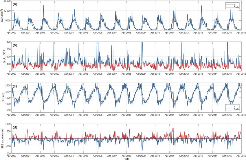
T. A. N. Redpath et al.: Clutha Catchment snow cover variability 3195
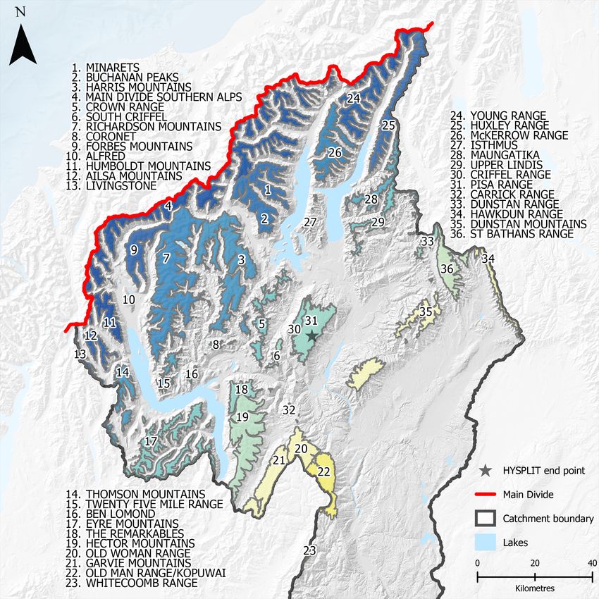
Figure 3. Individual mountain ranges mapped out within the Clutha Catchment for analysis of SCD variability and temperature and precip-
itation sensitivity. The end point for HYSPLIT back-trajectories is also shown. Elevation and relief data from Columbus et al. (2011); lakes
outlines and geographic place names are sourced from the LINZ Topographic Database.
Table 1. Basin-wide snow-covered area (bSCA) temporal metrics. These metrics were calculated annually, per pixel.
Name Description bSCA (%)
tSCD Total number of snow cover days 10, 15, 20
maxSCD Maximum continuous number of days exceeding fSCAt 10, 15, 20
maxSCDonset First day of maxSCD 10, 15, 20
maxSCDloss Last day of maxSCD 10, 15, 20
The temporal component of variability, however, may not dered according to the proportion of overall variance they ex-
be readily interpreted from this “atmospheric science PCA” plain. Conceptually, this approach, which can be considered
(Demšar et al., 2012). as “raster PCA” (rPCA) (Demšar et al., 2012) is analogous to
When applied to spatio-temporal data, such as time series the application of PCA to multispectral imagery, where PCs
of raster maps capturing a spatially continuous variable, each are determined in a temporal, rather than spectral, attribute
principal component is a map representing a spatial mode of space. Spatialisation is a product of the geo-referenced raster
variability occurring within the time series. The PCs are or- datasets, and PCs are calculated only in the attribute space,
www.hydrol-earth-syst-sci.net/23/3189/2019/ Hydrol. Earth Syst. Sci., 23, 3189–3217, 2019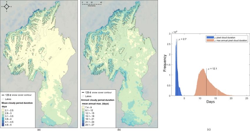
3196                                                         T. A. N. Redpath et al.: Clutha Catchment snow cover variability

so geographic effects are not accounted for (Demšar et al.,          matic gradients in the east of the South Island, owing to pre-
2012). A key benefit of the rPCA approach is that, when ap-          dominant westerly air flow and the substantial orographic ef-
plied to a raster time series, it allows the occurrence of spe-      fects of the Southern Alps (Sinclair et al., 1997; Jobst et al.,
cific modes of spatial variability to be considered as a func-       2018), the distance from each range to the Main Divide of
tion of time. Thus, the spatio-temporal variability within the       the Southern Alps was calculated using the Near tool in Ar-
data is preserved and can be further scrutinised and inter-          cGIS v10.3. Mean annual SCD anomalies for each range
preted.                                                              were then extracted from the maps calculated in Sect. 3.3.2.
   Here, rPCA was applied to the time series of SCD anomaly          Ranking each range in terms of proximity to the Main Divide
maps. The resulting PCs provide an indication of the spatial         then provided a basis for examining spatial trends in the SCD
and temporal variability in the SCD anomaly. PCA was car-            anomaly across the catchment from year to year.
ried out using MATLAB®. The single value decomposition
algorithm was applied to the time series of 16 SCD anomaly           3.5   Climatic influences on snow cover variability
maps, yielding as many PCs. The first six PCs were retained
as together they explained > 75 % of the total observed vari-        Beyond characterising the snow climatology for the Clutha
ance, while the remaining PCs become increasingly less spa-          Catchment, relating spatio-temporal variability in SCD to cli-
tially coherent and are of limited use for further analysis and      matic variability is central to better understanding climatic
interpretation.                                                      influences on seasonal snow in New Zealand. This was done
                                                                     firstly by assessing the sensitivity of the annual SCD anoma-
3.4.2   Temporal dynamics of spatial modes                           lies to annual temperature and precipitation anomalies. Fur-
                                                                     thermore, the role of atmospheric circulation was assessed by
Each PC from the rPCA described in Sect. 3.4.1 reveals spa-          considering airflow as characterised by multiple atmospheric
tial modes of variability. In turn, the respective loadings of       back-trajectories generated for the study period using the Hy-
each PC can be used to identify years which share similarities       brid Single-Particle Lagrangian Integrated Trajectory (HYS-
in the spatial expression of their SCD anomalies. Comparing          PLIT) model (Stein et al., 2015). Airflow analysis was mo-
years based on their PCA signatures was done by consider-            tivated in part by the suggestion that increased frequency of
ing the loadings of the first six PCs, which explained 77 %          southerly airflow can significantly suppress temperatures in
of the total variance in the spatio-temporal dataset. The PCA        New Zealand (Dean and Stott, 2009), but also because vari-
provided a six-dimensional loading space, within which the           ability in airflow can be expected to produce spatial variabil-
similarity between years was measured by the Euclidean dis-          ity in the delivery of precipitation to the Clutha Catchment.
tance and k-mean clustering.                                            Several climatic datasets were acquired to investigate the
                                                                     role and relative influence of climatological processes in con-
3.4.3   Mountain range analysis                                      trolling the variability of seasonal snow, namely the follow-
                                                                     ing:
An alternative, semi-distributed approach was considered for          1. Gridded temperature and precipitation fields, compris-
characterising spatial variability in SCD. Addressing space              ing daily Tmax , Tmin , Tmean and Ptot for the period 2000–
via individual mountain ranges provided a basis to explore               2016, interpolated at a resolution of 250 m, coincident
spatial gradients in SCD variability across the catchment.               with the pixel size of comparable MODIS datasets, pro-
This approach allows the catchment to be treated in a way                duced as detailed in Jobst et al. (2017) and Jobst (2017).
that may be more readily understood by stakeholders, poten-              In the case of temperature, gridded data were produced
tially including industrial and agricultural water managers              from a limited observational network using a trivariate
and consumers, ski area operators, and the general public.               spline that was enhanced using process-driven lapse rate
Such stakeholders typically consider the snow resource at a              models (Jobst et al., 2017). Precipitation was also inter-
sub-catchment mountain range scale. The goal of this analy-              polated using a trivariate spline, with a 30-year normal
sis was to determine whether mountain ranges provide a use-              surface included as a covariate (Jobst, 2017).
ful geographic unit for capturing and characterising spatial
variability. The catchment was subdivided into 36 different           2. Monthly values of the Southern Oscillation In-
mountain ranges, based on the naming conventions provided                dex (SOI), and Southern Annular Mode (SAM,
by the 1 : 50 000 scale NZ Geographic Names topographic                  also known as the Antarctic Oscillation Index,
dataset (LINZ, 2017). All land areas below the median winter             AAO), from the NOAA National Weather Ser-
snow line elevation (as calculated in Sect. 3.3.3) of 1270 m             vice Climate Prediction Center (CPC). Data were
were excluded. Then, areas of mountain ranges above this                 sourced from https://www.cpc.ncep.noaa.gov/products/
elevation were manually digitised using a DEM (Columbus                  precip/CWlink/daily_ao_index/aao/aao_index.html
et al., 2011) and stream centre-line vector data (Snelder et al.,        (last access: 27 July 2017) (SAM) and https:
2010) as guidance (Fig. 3). Since the Main Divide of the                 //www.cpc.ncep.noaa.gov/data/indices/soi (last ac-
Southern Alps is considered to provide a baseline for cli-               cess: 28 June 2017) (SOI).

Hydrol. Earth Syst. Sci., 23, 3189–3217, 2019                                      www.hydrol-earth-syst-sci.net/23/3189/2019/
T. A. N. Redpath et al.: Clutha Catchment snow cover variability                                                              3197

Figure 4. Maps of the mean duration of cloud occurrence (a), mean of the maximum annual cloud occurrence duration (b) and histograms
of both (c). Lake outlines are sourced from the LINZ Topographic Database.

 3. Global gridded (2.5◦ ) NCEP/NCAR meteorological re-             3.5.2   Synoptic-scale airflow variability
    analysis data (Kalnay et al., 1996), used as input fields
    for the HYSPLIT (version 4) model. Data were acquired
                                                                    HYSPLIT is a Lagrangian air parcel trajectory and dispersion
    from the Climate Data Center (CDC) via the FTP mod-
                                                                    model (Stein et al., 2015). While it offers complex simula-
    ule within the HYSPLIT software.
                                                                    tions of particle atmospheric transport, dispersion, chemical
                                                                    transformation and deposition, the trajectories modelled by
3.5.1   Spatial anomalies for temperature and                       HYSPLIT provide a means to characterise airflow and asso-
        precipitation                                               ciated air-mass characteristics. Here, HYSPLIT was used to
                                                                    determine and analyse the origin and trajectory of air parcels
The daily fields of mean temperature and total precipitation        arriving to the Clutha Catchment throughout the study pe-
described above were used to calculate pixel-wise mean val-         riod.
ues for each hydrological year, as well as for each winter             The geographic end-point for the trajectories was a loca-
period. Winter was defined as being from 1 May to 30 Octo-          tion near the summit of the Pisa Range (Fig. 3), with eleva-
ber, the period during which the majority of substantial snow-      tion set to 2000 m. This location was close to the geographic
fall events occur. Pixel-wise anomalies in annual mean tem-         centre of the Clutha Catchment (−44.90◦ S, 169.16◦ E;
perature and total precipitation were calculated to produce         Fig. 3) and therefore expected to provide a suitable character-
a series of 16 anomaly maps for each variable, which were           isation of modes of air flow affecting the catchment through-
compared directly with the SCD anomaly maps. No signif-             out the year. Back-trajectories were calculated over 120 h for
icant correlation existed between temperature and precipita-        each day of the study period, with four temporal end-points
tion anomalies.                                                     per day (00:00, 06:00, 12:00, 18:00 New Zealand Standard
   The sensitivity of SCD anomalies to temperature and pre-         time, NZST). In total this provided 1460 trajectories per year.
cipitation anomalies was assessed in a semi-spatially dis-             HYSPLIT trajectories were used to construct indices of
tributed way. Regression analysis was carried out between           air-mass origin. For four timesteps, namely −96, −72, −48
the annual SCD anomaly and temperature and precipitation            and −24 h, the trajectory direction relative to the end-point
anomalies averaged over each mountain range. Sensitivity of         was determined and binned according to eight directional
SCD to temperature and precipitation variability could then         classes (i.e. N, NE, E, SE, S, SW, W, NW). This allowed
be quantified and its significance assessed for each mountain       the mean frequencies of air parcel origin direction and rela-
range across the catchment.                                         tive frequencies for each winter (1 June–30 September) pe-

www.hydrol-earth-syst-sci.net/23/3189/2019/                                      Hydrol. Earth Syst. Sci., 23, 3189–3217, 2019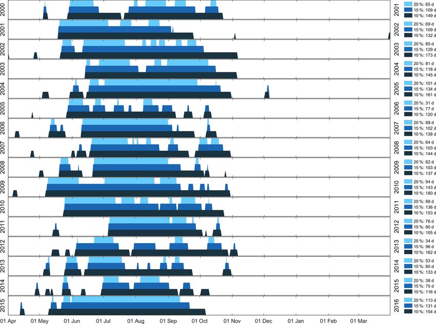
3198                                                          T. A. N. Redpath et al.: Clutha Catchment snow cover variability

Figure 5. Mean annual SCD (µSCD ) (a), and associated coefficient of variation, CV (CVSCD ) (b), for the Clutha Catchment, 2001–2016.
Elevation and relief data from Columbus et al. (2011); lake outlines are sourced from the LINZ Topographic Database.

riod to be calculated. The relative frequency distribution for        tance and significance of anomalous airflow directions to the
each winter then provided a means to characterise air-flow            modes of spatial variability in SCD to be assessed.
characteristics for each winter.
   Relationships between the annual loadings of each prin-            3.5.3   Assessing the role of climate modes
cipal component of SCD and the relative frequency of air
parcel origin direction were assessed by multiple linear re-          Commonly, short- to medium-term variability in climate and
gression. Because of the large number of variables (8) rela-          cryospheric processes in mid-latitude regions has been con-
tive to the number of years for which data exist (16), only           sidered in terms of large-scale climate modes such as the
four directions exhibiting the greatest inter-annual variabil-        SOI, the SAM and the Pacific Decadal Oscillation (PDO)
ity were included in multiple linear regression to mitigate           (e.g. McKerchar et al., 1998; Fitzharris et al., 2007; Kidston
against under-determination. This means that, for each prin-          et al., 2009; Purdie et al., 2011; Sirguey et al., 2016). Periods
cipal component (n) and each year (y), the linear model took          of negative SOI phase are expected to correspond with cooler
the following form:                                                   periods of increased solid precipitation in New Zealand, and
                                                                      have been associated with positive mass balance for glaciers
                                                                      in the Southern Alps (McKerchar et al., 1998; Lamont et al.,
λn(y) = β0(y) + β1(y) x1(y) + β2(y) x2(y)
                                                               (5)    1999; Fitzharris et al., 2007; Purdie et al., 2011), yet its inclu-
       + β3(y) x3(y) + β4(y) x4(y) ,                                  sion as a predictor variable does not necessarily increase the
                                                                      skill of hydrological forecast models (Purdie and Bardsley,
where λn(y) is the loading of the nth PC for that year, and           2010). Here, mean winter values of the SOI and SAM indices
β0(y) , . . ., β4(y) and x1 , .., x4 are the SCD sensitivity to and   were compared to each of the temporal metrics characteris-
relative frequency of air parcels originating in the NE, E,           ing snow cover within the catchment (Table 1) via correlation
SE and S. This analysis allowed the contribution, impor-              analysis and linear regression. The PCA analysis proposed

Hydrol. Earth Syst. Sci., 23, 3189–3217, 2019                                       www.hydrol-earth-syst-sci.net/23/3189/2019/
T. A. N. Redpath et al.: Clutha Catchment snow cover variability 3199
Figure 6. A 10 d moving average of daily snow-covered area (SCA) (a) and snowline elevation (SLE) (b). The mean of each is shown
in black, accompanied by the envelopes of associated standard deviation and range (illustrating the spread of trajectories), as well as the
standard error (representative of the uncertainty of the mean).
by this study provides new insights into the spatial expression 2200 m a.s.l. Considering the detection limits of MODIS, this
of snow cover variability that also deserves further scrutiny. area agrees well with the glacier area of Brunk and Sirguey
Subsequently, the influence of large-scale circulation indices (2018). These areas are largely restricted to within a few
on spatial modes of snow cover was explored by analysing kilometres of the Main Divide. The importance of aspect in
the correlation between the SOI and SAM and annual PC maintaining permanent snow cover for these high-elevation
loadings. regions is highlighted in Fig. 6.
The onset of the snow season is typically rapid, with SCA
increasing and SLE lowering abruptly in the early winter,
4 Results reaching their maximum and minimum, respectively, in mid-
June (Fig. 6). At the catchment scale, both SCA and SLE
4.1 Snow cover climatology for the Clutha Catchment feature a mid-winter depletion and rising respectively, be-
fore SCA increases and SLE decreases again in late winter
The snow cover climatology for the Clutha Catchment is ex- to early spring. Maximum SCA typically reaches > 35 % of
pressed spatially by the map of µSCD over the period 2000– the catchment area during June, yet the depletion curve is
2016. The first-order control of elevation on SCD is obvious punctuated by local maxima. On average, the first of these
in Fig. 5a. On average, an area of 2218 km2 , or 10 % of the occurs in early July, and the second in mid-August. These
total catchment area, maintains snow cover for 120 d a year features are persistent throughout the 16-year study period.
or more. In general, snow cover is most persistent on terrain In addition, a minima in variability of daily SCA occurs in
above 1500 m a.s.l., and on slopes with a southern aspect. late April, following an increase in variability due to early
The mean SLE during the winter period was found to be snowfall over the preceding month. Variability in basin SCA
1263 m a.s.l; this corresponds with an area of 3180 km2 and and SLE is greatest during the May–July period and con-
is substantially higher than the mean catchment elevation verges towards the mean through spring and early summer.
of 615 m. On average, the snowline is at or below this el-
evation from mid-June until mid-August (Fig. 6). A small
area of 76 km2 maintains permanent snow cover (SCD >
360 d). This corresponds with a maximum SLE of around
www.hydrol-earth-syst-sci.net/23/3189/2019/ Hydrol. Earth Syst. Sci., 23, 3189–3217, 20193200 T. A. N. Redpath et al.: Clutha Catchment snow cover variability
σ ) (b, d) as a function of aspect (a, b), and elevation (c, d). For clarity,
Figure 7. Mean SCD (a, c) and associated coefficient of variability ( µ
a random sub-sample of 50 000 pixels is displayed in the plots.
4.2 Topographic controls on snow duration and higher on southerly than northerly aspects (Fig. 7). A CVSCD
variability < 10 % is generally restricted to southerly aspects above
1500 m. Elsewhere, variability in SCD is relatively large.
Figure 7 shows the overall control of aspect and elevation on CVSCD increases markedly at lower elevations reflecting the
SCD and its variability. Most pixels exhibiting µSCD > 120 d relatively short µSCD and associated large inter-annual vari-
have a southerly aspect between 90 and 315◦ and elevation ability.
in excess of 1500 m. The role of aspect strengthens as eleva-
tion decreases. The variability in SCD is more pronounced 4.3 Spatio-temporal variability in seasonal snow cover
on northerly aspects between 315 and 90◦ , across all eleva-
tions. In contrast, the CVSCD rarely exceeds 100 % for pixels The map of CVSCD shown in Fig. 5b highlights the magni-
with S to SW aspect between 135 and 270◦ , but may exceed tude of spatio-temporal variability associated with SCD in
200 % for pixels with northerly aspect between 315 and 90◦ the Clutha Catchment. A first-order control of elevation on
(Fig. 7). CVSCD is apparent, but further spatial variation exists beyond
µSCD is positively, though not linearly, correlated with the basin hypsometry. Areas with CVSCD ≤ 5 % were only
elevation. The rate of increase of µSCD with elevation is present on and near the Main Divide, while CVSCD is much
Hydrol. Earth Syst. Sci., 23, 3189–3217, 2019 www.hydrol-earth-syst-sci.net/23/3189/2019/T. A. N. Redpath et al.: Clutha Catchment snow cover variability 3201
Figure 8. A 5 d moving average of daily snow-covered area (SCA) and percentage of mean snow-covered area for all years (a, b), and daily
snowline elevation (SLE) and daily SLE anomaly (c, d). Mean daily values, repeated for each year, are shown in grey in the daily SCA and
SLE plots.
greater elsewhere in the catchment. At moderate to high el- sion on which SCA exceeded 60 % of catchment area was
evations, CVSCD in the western part of the catchment was 21 June 2013. Notably, the years that feature the largest max-
generally less than 50 %. In the eastern part of the catchment, imum SCA values are not always associated with a sustained
CVSCD was generally greater, but this reflects the basin hyp- positive anomaly in catchment-wide SCA.
sometry to an extent. Ultimately, the large CVSCD observed The considerable temporal variability associated with
across most of the catchment reflects the temporally dynamic SCA is further demonstrated by the bSCA metrics plotted
nature of snow cover across the Clutha Catchment. in Fig. 9. The total number of days each year with bSCA ex-
ceeding 10 %, 15 % and 20 % is highly variable from year
4.3.1 Temporal variability in catchment-wide snow to year and did not reveal any significant trend over the 16-
cover and snowline elevation year time series. The lowest returned p value (0.23) was as-
sociated with a negative trend for the end date of temporally
continuous 15 % bSCA. Typically, 10 % bSCA is achieved
The full time series of daily SCA and SLE and associated de-
by June, with the latest onset date of 6 July occurring for HY
partures from their series means reveal the extent of temporal
2012. Generally, 10 % bSCA is sustained through 30 Septem-
variability in seasonal snow at the catchment scale (Fig. 8).
ber, resulting in a mean 120 d duration. The earliest end date
Substantial departures from the mean throughout the time
for 10 % bSCA, 8 September, occurred for HY 2006. Several
series highlight the strong inter-annual as well as shorter-
years saw 10 % bSCA extend through, or beyond, 31 Octo-
term variability in the occurrence, persistence and disappear-
ber. For HY 2010, an early onset of continuous 10 % bSCA
ance of seasonal snow within the catchment. Large, yet short-
(7 May), combined with a loss date of 30 September, resulted
lived, perturbations occur due to unseasonable snow events,
in the longest continuous duration of 10 % bSCA, of 176 d.
while sustained positive and negative anomalies occur at sea-
Both 15 % and 20 % bSCA saw much more variability,
sonal scales during winter. The maximum observed SCA was
with the period of 20 % bSCA being discontinuous for most
65 % and occurred on 18 June 2002. The only other occa-
www.hydrol-earth-syst-sci.net/23/3189/2019/ Hydrol. Earth Syst. Sci., 23, 3189–3217, 20193202 T. A. N. Redpath et al.: Clutha Catchment snow cover variability
Figure 9. Timeline of occurrence of 10 %, 15 % and 20 % basin snow-covered area (bSCA) for the Clutha Catchment for hydrological years
2001–2016.
winters. Onset of both 15 % and 20 % bSCA typically oc- of the total observed spatial variability in the annual SCD
curred within a few days of 10 % bSCA; however, there was anomaly was explained by the first six principal compo-
usually considerable lag between the end date of 15 % and nents (Fig. S1 in the Supplement). In turn, each annual SCD
20 % bSCA and that of 10 % bSCA. anomaly map can be efficiently reconstructed via linear com-
The winter SLE also exhibited significant intra- and inter- bination of each map of PC scores. As such, the loadings
annual variability, both in terms of the mean (median) win- of the combination quantify the relative contribution of each
ter SLE of 1263 m (1270 m), and the range of observed SLE mode to the SCD map. Since PC scores are not standard-
(Figs. 8 and 10). The largest ranges of observed winter SLE ised, their unit matches that of the SCD anomaly (i.e. day).
(e.g. HY 2012), were associated with years when the on- Where loadings are positive (negative), a positive PC score
set of winter snow cover was delayed. This scenario reflects will propagate positively (negatively) into the SCD anomaly.
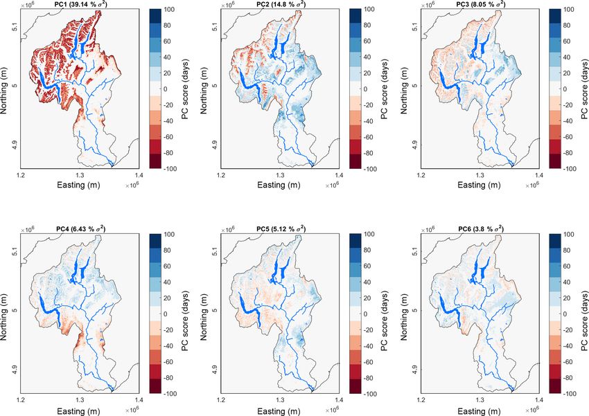
an over-representation of high SLE through June, which is PC1 (39 % of total variability), is characterised by a nega-
the month when the lowest SLE values are usually observed tive PC score across the whole catchment that reflects the
across the entire record. Similarly to SCA, no significant first-order control imposed on SCD by elevation (Fig. 11).
temporal trend was detected in SLE over the 16-year record. PC2 (14.8 % of total variability) features an annular pat-
tern expressed across much of the catchment, where nega-
4.3.2 Modes of spatial variability tive PC scores are associated with high-elevation areas, while
positive scores occur for lower-elevation areas, and in the
east of the catchment. Overall, PC2 highlights the existence
Mapping the principal components of the SCD anomaly re-
of a spatial trend in variability that departs from the topo-
vealed distinct modes of spatial variability (Fig. 11). 77 %
Hydrol. Earth Syst. Sci., 23, 3189–3217, 2019 www.hydrol-earth-syst-sci.net/23/3189/2019/T. A. N. Redpath et al.: Clutha Catchment snow cover variability 3203
Figure 10. Box plots of winter (1 June–30 September) snowline elevation for all years. The upper and lower bounds of the boxes are the
75th and 25th percentiles, respectively. Outliers are represented by “+” symbols.
Table 2. The k-means clusters based on principal component load- 4.3.3 Dynamics of spatio-temporal variability
ings of SCD anomalies.
The attribute space of annual PC loadings facilitated the com-
Cluster parison and grouping of years in terms of the spatial structure
of their SCD anomaly. The two most similar years, in terms
1 2 3 4
of PC loadings, were 2015 and 2006, while the two most
2007 2002 2001 2003 dissimilar were 2010 and 2007 (Fig. 12). PC1 (38 % of spa-
2009 2006 2004 2005 tial variability) carried relatively strong positive loadings for
2011 2013 2008 2010 hydrological years 2002, 2006, 2012, 2014 and 2015, while
– 2015 2012 2016 negative loadings for PC1 were associated with 2003, 2005,
– − 2014 –
2010 and 2016. The relatively large pair-wise distances be-
tween PC loadings for most years (Fig. 12) illustrates that,
over the 16-year period, the spatial structure of the SCD
graphic control characterised by PC1. PC3 (8.05 % of to- anomaly across the catchment is rarely repeated, except in
tal variability) further stresses a spatial trend, with negative 2006 and 2015. As a result, groups identified by k-mean clus-
PC scores in the west transitioning to positive scores in the tering of their PC loading signature are potentially weak. As-
Manuherikia (north-east) region of the catchment, and for signment into four clusters performed well at grouping the
higher elevations in the central part of the catchment (e.g. most similar years together, whilst mitigating against single-
the Pisa Range). PC4 (6.43 % of total variability) also exhib- member clusters, and yet spurious members remain in all
ited spatial structure, with positive PC scores in the north of clusters (Table 2 and Fig. 12).
the catchment, and negative scores dominating south of the
Kawarau and Manuherikia rivers. Explaining 5.12 % of total 4.3.4 Spatio-temporal variability in SCD across
variability, PC5 shows that SCD anomalies are further mod- mountain ranges
ulated by spatially structured contrasts between negative PC
scores in the central part of the catchment, and positive scores A semi-distributed analysis of the SCD by mountain range
through the western, northern, and eastern margins. Finally, provides further insight into spatial variability of SCD within
PC6 (3.8 % of total variability) exhibits weaker spatial struc- the catchment. Since the mean elevation varies for each
ture, with positive PC scores through most of the western part mountain range, the influence of elevation on SCD could
of the catchment, and at low to moderate elevations towards be assessed. The mean annual SCD of individual mountain
the east. Negative stores occur at higher elevations in central ranges is shown in Fig. 13, which demonstrates that average
and eastern areas. The magnitude of scores was reduced for SCD is a function of elevation, as well as proximity to the
PC6 relative to PCs 1–5. PCs 7–16 each explained less than Main Divide. For ranges within 60 km of the Main Divide, a
3 % of total variability. significant positive correlation exists between mean range el-
evation and SCD, with the modelled relationship predicting
an elevation of 2298 m for perennial snow cover. Beyond dis-
tances of 60 km from the Main Divide, however, the relation-
www.hydrol-earth-syst-sci.net/23/3189/2019/ Hydrol. Earth Syst. Sci., 23, 3189–3217, 20193204 T. A. N. Redpath et al.: Clutha Catchment snow cover variability
Table 3. Robust (bi-square) regression parameters between mean elevation and mean SCD for mountain ranges within the Clutha Catchment.
Regression was carried out for all ranges together, and for those ranges within 60 km of the Main Divide and those more than 60 km from
the Main Divide.
Ranges n β (d m−1 ) c R2 RMSE p
All 36 0.24 −246.11 0.50 24.8 0.00
< 60 km of M.D. 24 0.32 −370.52 0.74 20.3 0.00
> 60 km of M.D. 12 0.07 3.89 0.07 25.1 0.41
Figure 11. The first six spatial principal components of the SCD anomaly.
ship weakens substantially and loses significance (Table 3). tial gradients of the SCD anomaly observed for these years,
The deterioration of the relationship between elevation and from west to east, are consistent with the derived principal
SCD for ranges distant from the Main Divide suggests that components. PC2 and PC3, in particular, characterised the
the influence of temperature on SCD is substantially reduced east–west gradient in the SCD anomaly which typifies these
in these cases. “out-of-phase” years. Both of these principal components ex-
For 4 out of the 16 winters analysed (25 %), the sign of pressed an east–west contrast in SCD anomaly, with PC2
the anomaly was out of phase across the catchment. For the emphasising an inverted topographic dependency. The win-
winters of 2000 and 2003, the SCD anomaly was positive in ter of 2001 loaded negatively on PC2, while the winter of
the west and negative in the east, while the winters of 2008 2003 loaded negatively on both PC2 and PC3. Conversely,
and 2010 were negative in the west and positive in the east. the winters of 2008 and 2010 loaded positively on both PC2
These similarities are consistent with these pairs of years be- and PC3, with 2010 being the only winter to load strongly
ing grouped together on the basis of PC loadings. The spa- on both of these PCs. The consistent signal between PC sig-
Hydrol. Earth Syst. Sci., 23, 3189–3217, 2019 www.hydrol-earth-syst-sci.net/23/3189/2019/T. A. N. Redpath et al.: Clutha Catchment snow cover variability 3205
Figure 12. (a) Loadings for the first six principal components of the SCD anomaly (77 % of total variance) for each hydrological year (which
corresponds with the winter of the preceding calendar year). (b) Normalised distance between PC loadings.
natures and the range anomaly approach demonstrates that and temperature anomaly. For all ranges, β was negative,
both the fully distributed and range-based semi-distributed with the greatest sensitivity of −53.6 d ◦ C−1 occurring for
approaches are consistent in detecting variability in spatial the Ailsa Range. For precipitation, a significant relationship
contrasts. It also highlights that snow cover conditions across with SCD was found for 39 % of ranges. Values of β were
the Clutha Catchment are often spatially out of phase, with always positive, with a maximum sensitivity of 0.11 d mm−1
first-order control by elevation being of diminished impor- occurring for the Eyre Mountains.
tance. This out-of-phase behaviour, and indeed the variabil- Sensitivity of the SCD anomaly to both temperature and
ity in magnitude anomaly even when the entire catchment is precipitation anomalies was considered in terms of both ele-
in phase, confirms that processes at the sub-catchment scale vation and proximity to the Main Divide and exhibited sig-
are important in controlling variability in seasonal snow pro- nificant spatial trends (Figs. 15 and 16). Figure 15 reveals
cesses, and that influence of and sensitivity to competing cli- that distance to the Main Divide outperforms elevation at ex-
matic forcings varies across the catchment. plaining variability in sensitivity to temperature. In the case
of precipitation sensitivity, no relationship is evident with el-
4.4 Climatic influences on SCD evation, while a complex relationship with distance to the
Main Divide is apparent.
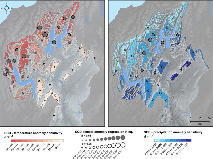
4.4.1 Sensitivity of SCD to temperature and Maximum temperature sensitivity occurred on and near
precipitation variability the Main Divide, reducing at a rate of 0.43 d ◦ C−1 km−1 east-
ward from the Main Divide, concurrently with decreasing R 2
Regression analysis between SCD, winter temperature and and increasing p values. The relationship between tempera-
winter precipitation anomalies revealed a variable response ture anomaly and SCD anomaly becomes insignificant be-
across the catchment. Sensitivity to temperature and precipi- yond distances of 55 km from the Main Divide. For precip-
tation variability is expressed as days (d) per degree Celsius, itation, a more complex spatial trend emerged, whereby the
or mm, respectively. Overall, relationships between tempera- relationship with SCD anomaly was weak and insignificant
ture and precipitation anomalies and the SCD anomaly were for ranges on and near the Main Divide, before becoming
found to be significant (p < 0.05) across the catchment, yet significant and strengthening with distance between 20 and
both regressions featured high dispersion, with R 2 = 0.19 for 55 km, where the strongest significant relationship occurred.
temperature and R 2 = 0.11 for precipitation (Table S2). This From this point, sensitivity to precipitation, as well as the
dispersion was found to be due to contrasting climatic sensi- strength of the relationship, decreased. The relationship be-
tivity across the catchment. For temperature, 50 % of ranges tween precipitation and SCD anomaly was insignificant at
exhibited a statistically significant relationship between SCD distances greater than 80 km from the Main Divide.
www.hydrol-earth-syst-sci.net/23/3189/2019/ Hydrol. Earth Syst. Sci., 23, 3189–3217, 2019You can also read