Central Himalayan tree-ring isotopes reveal increasing regional heterogeneity and enhancement in ice mass loss since the 1960s - The Cryosphere
←
→
Page content transcription
If your browser does not render page correctly, please read the page content below
The Cryosphere, 15, 95–112, 2021
https://doi.org/10.5194/tc-15-95-2021
© Author(s) 2021. This work is distributed under
the Creative Commons Attribution 4.0 License.

Central Himalayan tree-ring isotopes reveal increasing regional
heterogeneity and enhancement in ice mass loss since the 1960s
Nilendu Singh1 , Mayank Shekhar2 , Jayendra Singh3 , Anil K. Gupta4 , Achim Bräuning5 , Christoph Mayr5 , and
Mohit Singhal1
1 Centre  for Glaciology, Wadia Institute of Himalayan Geology, Dehradun 248001, India
2 Birbal  Sahni Institute of Palaeosciences, Lucknow 226007, India
3 Wadia Institute of Himalayan Geology, Dehradun 248001, India
4 Department of Geology and Geophysics, IIT Kharagpur, Kharagpur 721302, India
5 Institute of Geography, University of Erlangen–Nuremberg, 91058 Erlangen, Germany

Correspondence: Achim Bräuning (achim.braeuning@fau.de)

Received: 1 May 2020 – Discussion started: 25 June 2020
Revised: 31 October 2020 – Accepted: 6 November 2020 – Published: 6 January 2021

Abstract. Tree-ring δ 18 O values are a sensitive proxy for re-    1   Introduction
gional physical climate, while their δ 13 C values are a strong
predictor of local ecohydrology. Utilizing available ice-core      Glaciers in the Himalayan–Tibetan orogen are an important
and tree-ring δ 18 O records from the central Himalaya (CH),       component of the regional hydrological cycle, and a major
we found an increase in east–west climate heterogeneity            fraction of regional potable water is stored and provided by
since the 1960s. Further, δ 13 C records from transitional west-   them. However, recent climate warming has imposed a se-
ern glaciated valleys provide a robust basis for reconstruct-      rious alteration on the equilibrium of these glaciers (Bandy-
ing about 3 centuries of glacier mass balance (GMB) dynam-         opadhyay et al., 2019; Bolch et al., 2012; Maurer et al., 2019;
ics. We reconstructed annually resolved GMB since 1743 CE          Mölg et al., 2014; Yao et al., 2012; Zemp et al., 2019). High
based on regionally dominant tree species of diverse plant         uncertainty prevails in future projections of glacier mass bal-
functional types. Three major phases became apparent: pos-         ance (GMB), since sound understanding of glacier fluctua-
itive GMB up to the mid-19th century, the middle phase             tions and GMB response to climate change on multi-decadal
(1870–1960) of slightly negative but stable GMB, and an ex-        timescales is poorly understood (e.g. the erroneous statement
ponential ice mass loss since the 1960s. Reasons for acceler-      in the Fourth Assessment Report of the IPCC; Kargel et al.,
ated mass loss are largely attributed to anthropogenic climate     2011). Reliable projections of future Himalayan ice mass
change, including concurrent alterations in atmospheric cir-       loss require robust observations of glacier response to past
culations (weakening of the westerlies and the Arabian Sea         and ongoing climate change. Long-term estimation of GMB
branch of the Indian summer monsoon). Multi-decadal iso-           is also imperative for regional water security. Currently, cou-
topic and climate coherency analyses specify an eastward de-       pled glacier–climate models do not even agree on the sign
clining influence of the westerlies in the monsoon-dominated       of change, and hence projections of GMB are ambiguous
CH region. Besides, our study provides a long-term context         (Watanabe et al., 2019; Jury et al., 2019; DCCC, 2018). Nev-
for recent GMB variability, which is essential for its reliable    ertheless, a consistent picture emerges of net ice mass loss in
projection and attribution.                                        recent decades, which is highest in the western and central
                                                                   Himalaya (except the Karakoram and the Pamir Mountains)
                                                                   (Bolch et al., 2012; Brun et al., 2017; Dehecq et al., 2019;
                                                                   Maurer et al., 2019; Mölg et al., 2014; Shekhar et al., 2017;
                                                                   Yao et al., 2012).

Published by Copernicus Publications on behalf of the European Geosciences Union.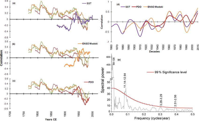
96                                                                    N. Singh et al.: Glacial history from central Himalaya

   The central Himalayan glaciers show a rather homoge-               The length of observed mass balance records princi-
neous behaviour (Azam et al., 2018; Bandyopadhyay et al.,          pally limits our understanding of the response of Himalayan
2019; Brun et al., 2017; Dehecq et al., 2019; Kääb et al.,         glaciers to climate change. Remote sensing techniques pro-
2012; Sakai and Fujita, 2017; Yao et al., 2012). In this study,    vide the best alternative in this regard (Garg et al., 2017,
we focus on the transitional climate zone between the west-        2019; Maurer et al., 2019; Kääb et al., 2012; Dehecq et al.,
ern and central Himalaya, where knowledge about multi-             2019; Brun et al., 2017; Bandyopadhyay et al., 2019; DCCC,
decadal glacier dynamics in relation to climate change is still    2018). Nevertheless, observation-based mass balance records
missing. Evidence from tree-ring isotopes and hydroclimatic        cannot be extended beyond a few decades. To understand
studies from the central Himalaya suggest that the glacier         long-term changes, we must rely on proxy data. One valu-
mass balance behaviour is primarily determined by the con-         able proxy is ice-core isotopes, which are yet to be obtained
joint effect of the winter westerlies (WD) and Indian summer       from the Indian Himalaya. Tree rings are another reliable and
monsoon (ISM) (Fig. 1 and references therein). The influence       sensitive proxy allowing the reconstruction of glacier history.
of the ISM declines towards the northwest Himalaya, and            They have been widely used in mountainous regions around
the westerlies progressively become dominant. Towards the          the world (Bräuning, 2006; Duan et al., 2013; Gou et al.,
eastern Himalaya, the influence of the Arabian Sea branch of       2006; Hochreuther et al., 2015; Larocque and Smith, 2005;
the ISM declines, and the Bay of Bengal branch dominantly          Linderholm et al., 2007; Nicolussi and Patzelt, 1996; Solom-
regulates the climate, besides an influence of the East Asian      ina et al., 2016; Tomkins et al., 2008; Watson and Luckman,
monsoon (Benn and Owen, 1998; Bookhagen and Burbank,               2004; Xu et al., 2012; Zhang et al., 2019). Tree-ring width
2010; Hochreuther et al., 2016; Liu et al., 2014; Lyu et al.,      (TRW) is known to bear the influence of non-climatic fac-
2019; Mölg et al., 2014; Sano et al., 2017; Yang et al., 2008;     tors like biological tree age, which overlap climatic signals
Yao et al., 2012). Monsoon-influenced glaciers, particularly       (Bunn et al., 2018; Zhang et al., 2019). TRW records of Hi-
those in the transitional climatic zone (such as the western re-   malayan evergreen conifer trees (including Cedrus deodara,
gion of the central Himalaya), are more sensitive to climate       Abies, Larix, and Picea spp.) have been widely used to recon-
warming than winter-accumulation type glaciers (Kargel et          struct hydroclimate and natural hazards (Borgaonkar et al.,
al., 2011; Sakai and Fujita, 2017). Moreover, a weakening in       2009, 2018; Cook et al., 2003; Singh et al., 2006; Singh and
the moisture-delivering systems (i.e. WD and ISM) since the        Yadav, 2013; Yadav and Bhutiyani, 2013; Yadav et al., 2011;
mid-20th century have had a direct impact on the summer-           Yadav, 2011). Despite numerous TRW-based climate recon-
accumulation type glaciers in the region (Qin et al., 2000;        structions, there is only one TRW-derived glacier mass bal-
Hunt et al., 2019; Joswiak et al., 2013; Khan et al., 2019;        ance reconstruction (Shekhar et al., 2017). Tree-ring stable
Roxy et al., 2015, 2017; Sano et al., 2012, 2013, 2017; Singh      isotopes are a reliable source of past hydroclimate variability
et al., 2019; Xu et al., 2018; Yadav, 2011).                       because of their sensitivity to local and regional climate, the
   In the present study, we attempt to reconstruct glacier mass    coherence in their climatic response, and the well-understood
balance history since the end of the Little Ice Age (since         control by the environmental conditions regulating tree phys-
1743 CE) in the transition zone between the ISM and the            iology (Levesque et al., 2019; Sano et al., 2012, 2013, 2017;
westerly-dominated climate in the western central Himalaya         Singh et al., 2019; Zeng et al., 2017). Although many studies
(Fig. 1). We use tree-ring stable-isotope (δ 13 C and δ 18 O)      have reconstructed hydroclimate in the Himalaya using tree-
chronologies of three dominant tree species of two different       ring isotopes (e.g. Sano et al., 2012, 2013, 2017; Singh et al.,
plant functional types and synthesize available regional δ 18 O    2019; Xu et al., 2018), glacier mass balance reconstructions
chronologies from different archives, including tree rings and     from tree-ring isotope series are still not available. Higher
ice cores across the central Himalaya (Fig. 1; Table S1).          growing-season temperatures stimulate photosynthesis rates.
   Field-based mass balance measurements are logistically          This facilitates a stable-isotope fractionation process, result-
challenging in the Himalaya. Nevertheless, since the 1980s,        ing in decreased intercellular CO2 concentration and frac-
workers have succeeded in monitoring four benchmark                tionation against the heavier 13 C isotope, which leads to in-
glaciers (Pratap et al., 2016; Garg et al., 2017, 2019) of the     creased δ 13 C. Thus, climate (temperature) is a bridge that
Uttarakhand Himalaya (Fig. 1). Based on a detailed anal-           indirectly connects the mass balance of a glacier with tree-
ysis of hypsometric curves and several morphological and           ring C isotope ratios. Hence, the mass balance can be recon-
glaciological factors of these four valley glaciers (Dokriani      structed using stable-carbon-isotope chronologies from trees
Glacier, DOK; Chorabari Glacier, CHO; Tipra Bamak, TIP;            growing in the proximity of the glacier (Zhang et al., 2019).
Dunagiri Glacier, DUN; Fig. 1, Table S2) (Bandyopadhyay               In this study, therefore, we utilized tree-ring carbon iso-
et al., 2019; Pratap et al., 2016; Garg et al., 2017, 2019) and    tope (δ 13 C) chronologies of three different species belonging
building upon previous studies (Shekhar et al., 2017; Bandy-       to two plant functional types (PFTs) that differ in their annual
opadhyay et al., 2019; Azam et al., 2018), we compiled a           phenological cycle (Table S1). One PFT includes evergreen
mean observed glacier mass balance time series starting in         conifers (Abies pindrow and Picea smithiana) that have been
the 1980s (1982–2013) (Figs. 1, S1; Table S2).                     widely used to reconstruct hydroclimatic regimes across the
                                                                   Himalaya and are abundantly found in the moist valley re-

The Cryosphere, 15, 95–112, 2021                                                         https://doi.org/10.5194/tc-15-95-2021
N. Singh et al.: Glacial history from central Himalaya 97
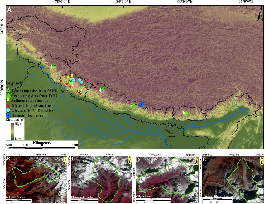
Figure 1. (a) The study region at the transitional climate zone of the western central Himalaya (WCH) showing tree-ring sampling sites,
meteorological and aethalometer stations, and four benchmark glaciers of the Uttarakhand Himalaya (b: Dokriani Glacier; c: Chorabari
Glacier; d: Tipra Bamak; e: Dunagiri Glacier). Tree-ring sites from the WCH include (1) Manali (Sano et al., 2017), (2) Uttarakashi (Singh
et al., 2019), and (3) Jageshwar (Xu et al., 2018). The Dasuopu ice core site in the eastern part of the central Himalaya (ECH) has been
indicated with a blue circle with a dot (Thompson et al., 2000), while tree-ring sites of the ECH are (5) Ganesh (Xu et al., 2018) and (6)
Bhutan (Sano et al., 2013). The fourth tree-ring site (Humla; Sano et al., 2012) has been indicated between the WCH and ECH.
gions of the high central Himalaya. Moreover, we investi- 2 Materials and methods
gated the dendroclimatological potential of a major domi-
nant species of broadleaf deciduous trees (Aesculus indica), 2.1 Study region and climate
as its growth period (April to September) coincides with the
warm–wet phase during the Indian summer monsoon (ISM) The present study focuses on the glaciers of the Uttarakhand
season (and lacks westerlies’ signal due to complete win- Himalaya (Indian central Himalaya) in the transitional cli-
ter dormancy). Additionally, we utilized available Dasuopu mate zone between the western and the central Himalaya.
ice core and tree-ring isotope chronologies from six different The study region extends from latitude 30.15 to 31.03◦ N
locations in the central Himalaya to substantiate our results and longitude 78.78 to 80.73◦ E. The highly glaciated up-
(Fig. 1). This study aims (i) to identify the tree-ring param- per reaches of the Uttarakhand Himalaya encompass about
eter (TRW and/or δ 13 C, δ 18 O) of deciduous and evergreen 1000 glaciers of varying size, which cover a total area about
tree species containing the strongest mass balance signature; 2850 km2 (Raina and Srivastava, 2008; Bandyopadhyay et
(ii) to reconstruct annual glacier mass balance using the iden- al., 2019). Previous studies have found that glaciers in the
tified best proxy chronology; and (iii) to analyse the recon- region are mainly fed by the ISM (Azam et al., 2018; Sakai
structed mass balance in relation to regional climate, local and Fujita, 2017). Therefore, glaciers in the region are usu-
forcing factors, and large-scale atmospheric circulation. ally classified as summer-accumulation type glaciers (Azam
et al., 2018; Sakai and Fujita, 2017). Snow accumulation
https://doi.org/10.5194/tc-15-95-2021 The Cryosphere, 15, 95–112, 202198 N. Singh et al.: Glacial history from central Himalaya
during winter (December–March) is influenced by a pre- well (Solomina et al., 2016). Ideally, land-terminated val-
cipitation regime driven by mid-latitude westerlies (WD). ley type glaciers of a simple configuration and hypsome-
Decadal-scale meteorological records from the study re- try are most suitable for inferring palaeoclimatic informa-
gion are available only for lower elevations (< 2000 m a.s.l.) tion (Solomina et al., 2016). The four studied glaciers are of
(Fig. 1). Therefore, long-term gridded temperature and pre- this kind and are therefore designated by workers as “bench-
cipitation datasets were obtained through the Climatic Re- mark glaciers”. The glaciers are of a similar small size (ex-
search Unit (CRU TS v. 3.22, 0.5 latitude × 0.5 longitude, cept DUN), have simple shapes, and have moderate eleva-
1901–2015) (Harris et al., 2014). However, given the lim- tion ranges, and thus their recent deglaciation responded to
itations of the CRU precipitation dataset in high-altitude changes in the climate equivalently (Table S2). A surface ice
regions, we complemented it with existing meteorological velocity study (Table S2) confirmed a similar response time
records (Singh et al., 2019). Analyses of meteorological of these glaciers (Garg et al., 2019). Geomorphological fea-
records indicate that mean annual precipitation is ∼ 800 mm, tures determining glacier hypsometry primarily regulate the
of which the warm–wet summer months (April–September) response of an individual glacier to changes in the climate.
receive about 80 %. Mean annual temperature varies around Thus, we prepared hypsometric curves of these four bench-
4 ◦ C, with a minimum (−7 ◦ C) in January and maximum mark glaciers (Fig. S1), which were convex for the DOK and
(13.5 ◦ C) in June (Fig. S2). As previously mentioned, stud- CHO glaciers and concave for the TIP and DUN glaciers.
ies indicate an increasing trend in temperature, while pre- These curves and other similar glacio-morphological indices
cipitation during both ISM and WD seasons show a recent (Garg et al., 2017, 2019) (Table S2) provide a reasonable
declining trend. As local climate is the common factor in- basis to compile these individual mass balance time series
fluencing both glacier mass balance and the physiology and (Shekhar et al., 2017; Bandyopadhyay et al., 2019).
growth of the trees growing in the valleys, we first analysed
tree growth–climate relations (Fig. S3). Averaged monthly 2.3 Tree-ring data
temperature and total monthly precipitation over a period
spanning October of the preceding year to September of the The three tree species utilized in this study are ubiquitously
current growth year were correlated with δ 13 C chronologies distributed throughout the western central Himalaya and
of the species (as δ 13 C is a strong predictor of local clima- have been used earlier to reconstruct past climatic variations.
tology) (Fig. S3). In addition, various climatological indices The collected species occupy both aspects of a glacier val-
(sea surface temperature, SST; the El Niño–Southern Oscil- ley, stretching from near the treeline to downslope towards
lation, ENSO; ENSO Modoki; the Pacific Decadal Oscilla- the valley. About 20 to 30 increment core samples of healthy
tion, PDO; and the Indian Ocean Dipole, IOD) were obtained tree individuals (to minimize the influence of non-climatic
from the archive (http://climexp.knmi.nl, last access: 23 Jan- factors on growth) were collected from higher-elevation sites
uary 2020) to analyse large-scale climatic relations. (2500–3800 m a.s.l.) from two representative glacial valleys
(Dokriani – DOK, Pindar – PIN) encompassing the basin
2.2 Glacier mass balance data in the Indian central Himalaya (Fig. 1). Tree-ring isotopic
signals (particularly δ 18 O) are coherent over a large area,
Four benchmark valley glaciers that are distributed across the as shown by high inter-species and inter-site correlations
Uttarakhand Himalaya, namely Dokriani (DOK), Chorabari in the Himalaya (Sano et al., 2012, 2013, 2017; Xu et al.,
(CHO), Tipra Bamak (TIP) and Dunagiri (DUN) glaciers, 2018; Grießinger et al., 2019; Table S1). Recently, Singh
have been individually monitored for their mass balance over et al. (2019) reconstructed regional ISM precipitation de-
the time period from 1982 to 2013 (with a few gap years; rived from δ 18 O chronologies of the same three tree species
Fig. 1, Table S2) (Pratap et al., 2016; Garg et al., 2017, from the DOK valley and found high inter-species and inter-
2019). Two glaciers (DOK and CHO) lie in the Garhwal Hi- site correlations. Due to the unavailability of long-term tree-
malaya, while two (DUN and TIP) are located in the Ku- ring stable-isotope records from PIN valley, we utilized δ 13 C
maun Himalaya (India). We used the available glaciological chronologies of the three tree species from the DOK valley.
mass balance records to produce the best possible time se- In summary, we adopted a methodology to reconstruct
ries (Table S2). We built a mean mass balance time series glacier mass balance history from tree rings that had been
based upon previous studies (Shekhar et al., 2017; Bandy- successfully tested before (Nicolussi and Patzelt, 1996;
opadhyay et al., 2019; Borgoankar et al., 2009) and the Duan et al., 2013; Zhang et al., 2019). We used stan-
premises that the glaciers show homogeneous behaviour in dard dendrochronological methods and techniques to de-
response to changes in the regional climate and that their velop tree-ring-width (TRW) and stable-isotope chronolo-
mass balances show a high inter-correlation (Azam et al., gies. Then, we calibrated the climate response using linear-
2018). Given the same climatic forcing owing to their lo- regression models and tested the reliability of our reconstruc-
cation in the humid central Himalaya and their similar ge- tion. The leave-one-out cross-validation method (LOOCV;
omorphological characteristics (Garg et al., 2017, 2019) (Ta- Michaelsen, 1987; Yadav and Bhutiyani, 2013; Duan et al.,
ble S2), the four valley glaciers should generally correlate 2013; Zhang et al., 2019) was used to verify our reconstruc-
The Cryosphere, 15, 95–112, 2021 https://doi.org/10.5194/tc-15-95-2021N. Singh et al.: Glacial history from central Himalaya 99
tion, given the relative shortness of glacier mass balance data surements. Isotope ratios are presented in the common δ no-
(23 years, 1982–2013 after omitting gap years of 1990–1992, tation against PDB as
1996, 1997, 2001–2003, and 2011) (Table S3).
13
C
12C sample
2.3.1 Tree-ring-width chronology development δ 13 C = − 1 × 1000 (‰).
13C
12C PDB
Two core samples per tree were collected at breast height
using 5.15 mm diameter increment corers. Standard den- The final tree-ring carbon isotope chronology was corrected
drochronological procedures (Fritts, 1976; Holmes, 1983) to incorporate isotopically light carbon released by the burn-
such as mounting and surface smoothing were applied to ren- ing of fossil fuels and increasing CO2 concentration, as pro-
der the ring boundaries clearly visible. TRW of the samples posed by McCarroll and Loader (2004) and McCarroll et
was measured at a resolution of 0.001 mm using a LINTAB™ al. (2009). The correction procedure applied here has the
system interfaced with a computer. Cross-dating was per- advantage of being objective, as it effectively removes any
formed by matching variations in ring widths in all cores declining trend in the δ 13 C series post 1850 CE, which is
to determine the absolute age of each ring. Dating and ring- attributed to the physiological response to increased atmo-
width-measurement quality control was conducted using the spheric CO2 concentrations (McCarroll et al., 2009).
COFECHA computer program (Holmes, 1983). A coherent
growth pattern between species revealed a common regional 2.4 Statistical analyses
climate signal affecting growth of the trees. However, TRW
chronologies of all species only showed a weak correlation Tree growth–climate relationships were analysed applying
with glacier mass balance data and hence were not used for simple Pearson correlation analysis. The relationship with
any reconstruction efforts. glacier mass balance was analysed using the pair-plot cor-
relation package “PerformanceAnalytics” (Carl et al., 2010)
2.3.2 Stable-carbon-isotope chronology development in R (Tables S4, S5; Fig. S3). Correlations were computed
between monthly temperature and rainfall data and the tree-
Five trees per species were selected for stable-isotope anal- ring δ 13 C chronology for a window from the previous year’s
yses based on best TRW inter-series matches. Each year’s October to the current year’s September.
growth rings were dissected with precaution with a sharp To better visualize the comparison between our recon-
scalpel under the microscope. To remove any possible ju- structed glacier mass balance time series and other hydro-
venile effect, the innermost approximately 30–40 rings of climatic reconstruction series from the monsoon-dominated
each tree core were omitted from the analyses. Wood sam- central Himalayan region (Fig. 1), data time series were stan-
ples were grounded using an ultracentrifuge mill (Retsch dardized using Z scores and smoothed with 11-year fast
ZM1). Extraction of cellulose from whole wood and car- Fourier transform to highlight common climate signals.
bon isotope analysis was carried out at the Institute of Geog- Based on correlation analysis, a linear-regression model
raphy, University of Erlangen–Nuremberg, Germany. Cellu- (Briffa and Jones, 1990; Cook et al., 1994) was used to
lose was extracted from the wood samples using the method perform the reconstruction using the lm module in R (gg-
of Wieloch et al. (2011). Isolated cellulose was homoge- plot2 package; Wickham, 2016). The leave-one-out cross-
nized using an ultrasonic method (Laumer et al., 2009) and validation method (LOOCV; Michaelsen, 1987) was used
freeze-dried. Before the pooling procedure, we checked co- for the entire calibration period (1982–2013) and to verify
relatedness in all five individual time series at 20-year inter- the reconstruction (Table S3). This method is most suitable
vals across the entire chronology. About 270 µg of cellulose when the length of observed records is short (Shah et al.,
was weighed into tin capsules with a microbalance (ME36S, 2013; Shekhar et al., 2017; Yadav and Bhutiyani, 2013; Ve-
Sartorius, Germany). The carbon isotope analyses were per- htari et al., 2017; Zhang et al., 2019). In this method, each
formed with an elemental analyser (NC 2500, Carlo Erba, observation is successively withdrawn, a model is estimated
Italy) linked to an isotope ratio mass spectrometer (IRMS; on the remaining observations, and a prediction is made
DELTAplus, Thermo Finnigan, Germany). Prior to isotope for the omitted observation. The LOOCV analysis was per-
analyses, samples were thoroughly dried in a vacuum-drying formed using the package “caret” (Kuhn et al., 2015). Rigor-
cabinet at 60 ◦ C. Isotope values were calibrated with inter- ous statistics, including the sign test, reduction in error (RE),
national (IAEA-CH-7, USGS41) and laboratory standards and correlation coefficients, were calculated to evaluate the
(peptone). The analytical precision was equal to or better similarity between observed and estimated values. The sign
than 0.2 ‰. Carbon (δ 13 C) values of samples were calculated test measures the degree of association between two series
by comparison with isotope-ratio-predetermined peptone and by counting the number of agreements and disagreements.
cellulose lab standards and certified international isotope The series are highly correlated if the number of similari-
standards (IAEA-601, IAEA-602, IAEA-CH-7, USGS41), ties is significantly larger than the number of dissimilarities.
which were inserted frequently in the course of sample mea- The RE statistic provides a rigorous test of the association
https://doi.org/10.5194/tc-15-95-2021 The Cryosphere, 15, 95–112, 2021100 N. Singh et al.: Glacial history from central Himalaya
between actual and estimated series. Any positive value indi- mean annual precipitation (MAP) remained similar (MAT
cates the predictive capability of the model. A positive RE is – Abies pindrow, r = −0.215, P < 0.05, n = 66; Aescu-
evidence of a valid regression model (Fritts, 1976). In addi- lus indica, r = −0.281, P < 0.05, n = 66; Picea smithiana,
tion, other rigorous statistics, viz. the root mean square error, r = −0.405, P < 0.001, n = 66), (MAP – Abies pindrow,
coefficient of efficiency (CE), and Durbin–Watson (DW) test r = 0.243, P < 0.05, n = 66; Aesculus indica, r = 0.115,
were carried out to evaluate the linear-regression model (Ta- P < 0.05, n = 66; Picea smithiana, r = 0.185, P < 0.05,
ble S3). n = 66). Results on monthly and seasonal climate-response-
Spatial and temporal correlations (moving correlations) function analyses are provided in the Supplement (Fig. S3,
were used to identify the coherence between reconstructed Table S5).
mass balance and gridded (0.5◦ × 0.5◦ ) temperature, pre- A weak correlation between TRW and glacier mass bal-
cipitation, SST, ENSO, ENSO-Modoki, PDO, and IOD for ance could arise due to sensitivity issues (Bunn et al., 2018).
the studied region in the central Himalaya. The variability At high elevations in a valley environment, temperature and
in the climate and glacier mass balance reconstruction in precipitation signals mix and make TRW records difficult to
the frequency domain was investigated using the multi-taper interpret (Bunn et al., 2019). In view of this, we resorted to
method (MTM) of spectral analysis (Mann and Lees, 1996) tree-ring isotopes (δ 13 C) of the species that are known to be
and wavelet transform (Grinsted et al., 2004) to identify pe- sensitive to climate. Interestingly, we found a strong corre-
riodicities and their temporal variability in the reconstructed lation only between δ 13 C of our studied conifer species and
data. compiled glacier mass balance (Abies pindrow, r = 0.596,
P < 0.001, n = 23; Picea smithiana, r = 0.631, P < 0.001,
n = 23). The correlations are strong enough to establish a
3 Results and discussion significant calibration model (Shah et al., 2013; Shekhar et
al., 2017; Yadav and Bhutiyani, 2013; Vehtari et al., 2017;
3.1 Annual glacier mass balance reconstruction Zhang et al., 2019). In contrast, correlation with the de-
ciduous species (Aesculus indica, r = 0.343, P = 0.1101,
The detailed results on the analysed relationship between n = 23) is weak during summer (April–September) and non-
δ 13 C and compiled glacier mass balance as well as of the significant during winter. This could be due to a lack of stor-
relationship between δ 13 C and available climate datasets are age of wintertime climate signals, as the species remains
presented in Tables S4 and S5. Descriptive statistics of δ 13 C physiologically active only during the wet–warm period from
chronologies and inter-species correlation (for the common April to September. Therefore, we utilized both evergreen
period) are shown in Table S1. Uncorrected and corrected conifer species for our reconstruction (Table S4). A linear-
δ 13 C chronologies (McCarroll and Loader, 2004) of the PFTs regression model was employed for the reconstruction of an-
are illustrated in Fig. S6. The mean difference in the iso- nual glacier mass balance (GMB) over the past 273 years,
topic composition of the two conifer species is ∼ 0.53 ‰ and the corresponding empirical equation is
(Abies pindrow, 1743–2015, −22.19 ± 0.7 ‰; Picea smithi-
GMB = 8.3984 + 0.3816 × δ 13 Cconifers .
ana, 1920–2015, −22.72±0.65 ‰). The mean δ 13 C value of
broadleaf deciduous species (Aesculus indica) is −24.31 ± Here, δ 13 Cconifers is the mean chronology of Abies pindrow
0.82 ‰. The difference (1.6 ‰–2.1 ‰) between δ 13 C time and Picea smithiana and GMB is annual glacier mass bal-
series of two PFTs indicates a higher level of isotope dis- ance (metre water equivalent, m w.e.). The detailed model
crimination in the broadleaf species relative to conifers. Fur- statistics are presented in Table S3. Model and calibration–
ther, break-point analysis indicated 1954 as a year of change verification statistics indicate the reliability and strength of
in the isotopic composition. Irrespective of the PFTs, a mean our reconstruction model (Table S3, Fig. S4; Fritts, 1976;
∼ 5 % decline in isotopic composition was noted after 1954 Vehtari et al., 2017). Validation tests including the number
relative to the pre-1950s level (Fig. S6). For the broadleaf of sign agreements between the reconstructed series and ob-
species, slopes of the trends for the periods prior and af- served mass balance records and the cross-correlation be-
ter 1954 are −0.001 and −0.032 ‰ yr−1 , respectively. For tween reconstruction and measurements are significant (P <
the conifers, they are −0.0007 and −0.025 ‰ yr−1 , respec- 0.001) (Fig. S4). However, the error estimates are based on
tively (P < 0.001). 113 C time series of broadleaf species measured mass balance data of only 23 years (1982–2013,
showed an increasing trend from 1954, with an average rate with a gap of a few years), so a possibility of uncertainty
of 0.15 ‰ yr−1 , while it remained stable for the conifers still exists in the reconstruction, particularly during the pre-
(0.003 ‰ yr−1 ) (Fig. S6). Nevertheless, a significant and pos- observation period. Nevertheless, the use of a sensitive iso-
itive inter-species correlation exists between them. This in- tope chronology (δ 13 C) and the combination of two conifer
dicates an influence of common and coherent climatic fac- species in this study may help to minimize several factors
tors on the physiological processes. Climate-response func- responsible for higher uncertainty, such as sensitivity issues,
tions indicate that for both PFTs, the correlation strength decreasing sample size, and temporal variability, which are
between δ 13 C and mean annual temperature (MAT) or unavoidable with TRW.
The Cryosphere, 15, 95–112, 2021 https://doi.org/10.5194/tc-15-95-2021N. Singh et al.: Glacial history from central Himalaya 101
3.2 Three major phases in the mass balance dynamics son et al., 2000; Kaspari et al., 2008; Denniston et al., 2000;
Kotlia et al., 2012, 2015; Liang et al., 2015) show that re-
Historical records of glacier change are rare from the Hi- gional climate has changed since the 1860s, with a reor-
malaya. However, available studies provide evidence that the ganization of hemispheric atmospheric circulation. Conse-
monsoon-influenced southeast Tibetan Plateau (TP) glaciers quently, the regional hydroclimate abruptly shifted towards
and those of the central Himalaya have responded syn- a drier phase concurrent with the changes in atmospheric cir-
chronously to the change in climate. In contrast, glaciers in culation. These records show a spatially coherent signal and
the western regions of the Himalaya–Tibet orogen have be- serve as a validation test of the accuracy of our GMB recon-
haved asynchronously (Solomina et al., 2016; Owen et al., struction (Fig. 2). Particularly, tree-ring and speleothem δ 18 O
2008; Kaspari et al., 2008; Liu et al., 2013; Hochreuther records (Singh et al., 2019, Sano et al., 2012, 2013, 2017; Xu
et al., 2015; Xu et al., 2012; Bräuning et al., 2006). Stud- et al., 2018; Kotlia et al., 2015; Liang et al., 2015) from our
ies highlight the relative importance of two moisture de- study region (Fig. 1) indicate increased westerly precipita-
livery systems (westerlies and Asian summer monsoon) in tion prior to 1860–1870 CE (Murari et al., 2014; Yang et al.,
driving regional glacier fluctuations; how variations in mois- 2008), which resulted in a phase of positive mass balance.
ture delivery systems have changed at millennial to glacial– Increased winter snowfall could be anticipated from a south-
interglacial timescales and their impact is even perceptible at ward shift in southwesterly winds due to reduced Northern
interannual to decadal timescales (Hou et al., 2017, Mölg et Hemisphere air temperatures during the LIA (Rowen, 2017).
al., 2014). The stronger influence of mid-latitude westerlies in driving
In a gross regional sense, the current state of the knowl- glacier variability in monsoonal high Asia (Mölg et al., 2014)
edge suggests that since the last glacier advance (LIA 1500– may have led to higher snowfall and positive mass balance
1850 CE) glaciers are in a general state of retreat, whereby prior to the 1870s as observed in our reconstruction (Fig. 2).
the role of regional climate in regulating regional glacier Regional temperature reconstructions (Zhu et al., 2011; Bor-
fluctuations has increased gradually (Mayewski and Jeschke, gaonkar et al., 2018; Yadav et al., 2011) also suggest a cold
1979; Mayewski et al., 1980). Therefore, across the Hi- and cloudy climate prior to 1850, which was followed by a
malaya this period (1850s onwards) is characterized by the warmer and sunnier climate thereafter (Liu et al., 2014; Xu et
dominancy of retreat, advance, and/or standstill regimes al., 2012). Indeed, a brief phase of a negative GMB trend dur-
(Mayewski and Jeschke, 1979; Mayewski et al., 1980; Bolch ing the 1770s to 1790s could be the result of warmer winter
et al., 2012; Rowan, 2017; Solomina et al., 2016). Avail- temperatures (Huang et al., 2019a) and below-average snow
able records from the central Himalaya indicate a state of accumulation during mega-droughts as observed around this
glacier retreat since the 1850s, regardless of the glacier type period (Cook et al., 2010; Thompson et al., 2000; Kaspari et
(Mayewski and Jeschke, 1979), with a recent acceleration in al., 2008) (Fig. 2). The close correspondence between recon-
ice mass loss as indicated by remote sensing studies (Maurer structed mass balance and regional hydroclimate reconstruc-
et al., 2019; Bandyopadhyay et al., 2019). tions supports the notion of hemispheric synchronicity to cli-
Our 273-year-long GMB reconstruction agrees with the mate change prior to 1860–1870 CE (Solomina et al., 2016).
general retreat of glaciers since the mid-19th century (Fig. 2). However, gradual changes in regional oscillations in temper-
Smoothing of the reconstruction with an 11-year moving av- ature and moisture delivery sources in the Himalaya–Tibet
erage and break-point analyses revealed three distinguish- orogen, particularly a change in the interplay of the ISM
able main phases: (1) a phase of positive mass balance up to and westerlies could have induced regionally distinguished
∼ 1870 CE, coincident with the LIA in the central Himalaya, climate zones with specific behaviour of glacier dynamics
(2) reorganization of Northern Hemisphere atmospheric cir- (Sect. 3.3).
culation following the LIA and a progressively increasing in- Glacial history during the late Holocene and LIA in our
fluence of regional climate could have resulted in a phase of studied region (Murari et al., 2014; Saha et al., 2019), and the
near-zero or stable mass balance that lasted up to the 1960s, above-mentioned proxy records and climate dynamics stud-
and (3) a phase of accelerated ice mass loss since the 1960s. ies (Mölg et al., 2014; Khan et al., 2019) indicate an out-
The latter phase corresponds to a global glacial retreat and of-phase relationship between the westerlies and ISM influ-
can be attributed to increasing temperatures, combined with ence. Therefore, regardless of the strength of the westerlies
a decline in ISM and westerly circulations and with anthro- (Joswiak et al., 2013), ISM weakening since the 1860s has
pogenic climate change (e.g. Bollasina et al., 2011). tended to shift the regional hydroclimate towards a drier and
Hydroclimatic evidence such as regional and composite a warmer climate. This could have favoured ice mass loss
tree-ring δ 18 O chronologies from the monsoon-influenced that led to a slightly negative mean mass balance (−0.046 ±
region (from southeast TP to central Himalaya) (An et al., 0.134 m w.e., ±SD) during the middle phase (1870–1959) in
2014; Singh et al., 2019; Grießinger et al., 2011; Wernicke our reconstruction. The timing of our reconstructed glacier
et al., 2017; Liu et al., 2014; Sano et al., 2012, 2013, 2017; advancement or recession is consistent with records of cold
Shi et al., 2012; Xu et al., 2018) and speleothems and the periods during the early 19th (1815–1825) and 20th (1900–
Dasuopu ice core record from the central Himalaya (Thomp- 1910) century (Zech et al., 2003). A brief period of declining
https://doi.org/10.5194/tc-15-95-2021 The Cryosphere, 15, 95–112, 2021102 N. Singh et al.: Glacial history from central Himalaya Figure 2. (a) Reconstructed glacier mass balance for the western central Himalaya (WCH) since 1743 CE (coloured inset indicates annual and pentadal mass change rate since the 1960s with SEs). (b) Annual snow accumulation record derived from Dasuopu ice core from the eastern central Himalaya (Thompson et al., 2000). Dark lines indicate 11-year moving averages. Vertical dashed lines are results of break-point analyses that reveal three major phases in the reconstruction. mass balance from 1865 to 1885 could be ascribed to warm to 1960–1985 (−0.275 ± 0.022 m w.e. yr−1 ). An extensive winter temperatures observed during 1848 to 1891 (Huang remote-sensing-based study encompassing the last 40 years et al., 2019a) and the late-Victorian intense drought dur- observed a consistent and similar trend of glacier loss ing 1875–1878 (Singh et al., 2018; Cook et al., 2010). The across the Himalayan transect (Maurer et al., 2019). For our slightly negative but stable mean GMB observed from 1920 study region, Bandyopadhyay et al. (2019) computed mean to 1960 is consistent with reported mass balances from the weighted mass balance as −0.61 ± 0.04 m w.e. yr−1 (2000– Himalaya (Bolch et al., 2012) and pluvial conditions from 2014), while we observed −0.65 ± 0.02 m w.e. yr−1 (exclud- enhanced ISM activity during 1920 to 1960 (Sinha et al., ing the very large-sized Gangotri Glacier). Similarly, several 2015). geodetic mass balance estimates from the western central Hi- Severe glacial mass loss (−0.437 ± 0.191 m w.e.) since malayan region are comparable (−0.4 to −0.8 m w.e. yr−1 ) the 1960s corresponds to a further and prominent shift to our results and are within the error limits of earlier stud- towards drier conditions arising out of the weakening of ies (DCCC, 2018; Bandyopadhyay et al., 2019; Maurer et al., both the ISM and westerlies (Qin et al., 2000; Hunt et 2019). al., 2019; Basistha et al., 2009; Singh et al., 2019; Sano In recent decades, along with the decreasing intensity of et al., 2012, 2013, 2017). Increasing regional and global moisture influx (ISM and WD), the importance of regional temperatures coupled with progressive regional industrial- temperature in regulating mass balance behaviour has been ization may have exacerbated the retreat rates. We ob- gradually increasing (Fig. 3). Several studies from the east- served a doubling of average ice mass loss rate (−0.577 ± ern Himalaya–Tibet orogen have emphasized the increased 0.022 m w.e. yr−1 ) (±SE) in the last 30 years compared influence of regional temperature in determining mass bal- The Cryosphere, 15, 95–112, 2021 https://doi.org/10.5194/tc-15-95-2021
N. Singh et al.: Glacial history from central Himalaya                                                                        103

ance behaviour (Bräuning, 2006; Yang et al., 2008). Our re-       India and ISM rainfall indicate a low association. However,
sults confirm historical observations made in the early 19th      we observed a high coherence (at both low and high fre-
century (without the availability of geochronological data        quencies) with local δ 18 O-reconstructed summer monsoon
to constrain the timing) that the central Himalayan glaciers      precipitation derived from several regionally dominant tree
have been receding since 1850 CE (Mayewski and Jeschke,           species (Singh et al., 2019) (Fig. 3a). Moreover, we also
1979; Rowen, 2017). The rate of ice mass loss has acceler-        found a tight correspondence with regional (Fig. 1) tree-ring
ated since the 1960s and almost doubled in the last 30 years      δ 18 O chronologies; the strength of which declined towards
with respect to pre-1985. Here, our results contradict the no-    the eastern central Himalaya (Fig. 3b, Table S6). Results in-
tion of UNEP (2009) that “despite the widespread shrink-          dicate an abrupt change in hydroclimate after the mid-20th
age of the Himalayan glaciers in area and thickness, the na-      century, which is particularly prominent in the western part
ture of shrinkage has not changed significantly over the last     of the central Himalaya. Moving correlations (51-year) be-
100 years” (UNEP, 2009).                                          tween GMB and tree-ring δ 18 O chronologies indicate a phase
                                                                  shift in the western part, which is more prominent relative to
3.3   Increasing regional heterogeneity                           the eastern central Himalaya after the 1960s (Fig. 3b).
                                                                     Regional tree-ring δ 18 O chronologies constitute sensitive
Substantial evidence exists from the monsoon-influenced           records that exemplify regional hydroclimatic heterogene-
Himalaya–Tibet orogen (Fig. 1) suggesting that LIA glacial        ity and show that the drivers of glacier fluctuations in the
fluctuations were more or less synchronous prior to 1850s         western part of the central Himalaya (WCH) are somewhat
(Hochreuther et al., 2015; Bräuning, 2006; Yang et al., 2008;     different from those in the eastern central Himalaya (ECH)
Xu et al., 2012; Mayewski and Jeschke, 1979; Rowen, 2017;         (Fig. 3b). Here, we contend that caution should be applied
Owen et al., 2008). Following the LIA, a global readjustment      when referring to the glaciers in the WCH as summer-
in atmospheric circulation resulted in a southward shift of the   accumulation type glaciers. We showed that over the WCH
Intertropical Convergence Zone (ITCZ). It broadly affected        (compared to the ECH), the westerlies still have a significant
the Asian summer monsoon, and the region has progres-             impact on annual mass balance behaviour. Earlier studies
sively moved towards a drier phase, subsequent to a break-        confirm that glaciers in the ECH and further east are mainly
down in the ITCZ and Northern Hemisphere temperature re-          fed by summer monsoon precipitation and thus are undisput-
lation since the mid-19th century (Ridely et al., 2015; Xu        edly classified as summer-accumulation type glaciers (Sakai
et al., 2012). Nevertheless, the strength of the westerlies in    and Fujita, 2017). However, our results reveal a contrasting
the region remained unaffected until the mid-20th century         hydroclimate relation between the WCH and ECH, with an
(Joswaik et al., 2013; Hunt et al., 2019; Khan et al., 2019).     opposite behaviour of moving correlation patterns (51-year)
Thus, depending upon the geographical location and prox-          between records of regional glacier–snow accumulation and
imity to the oceans, a distinct regionality developed, with a     tree-ring δ 18 O series (Fig. 4). When comparing the δ 18 O
decline in summer monsoon precipitation. The middle phase         chronology of the deciduous species (Aesculus indica, grow-
(mid-19th to mid-20th century) in our reconstructed GMB           ing in the WCH), we find the correlation pattern is strikingly
and in the annual snow accumulation recorded in the Da-           similar to that of the ECH, rather than to the WCH. In con-
suopu ice core supports this point of view (Fig. 2). During       trast to conifer species that take up meltwater containing win-
this period, cryospheric mass balance turned slightly nega-       ter precipitation isotopic signals in the early growing season
tive, with a gradual decline in summer precipitation, which       (Huang et al., 2019b), the broadleaf deciduous species takes
was more prominent towards the western part (Figs. 2, 3).         up soil water mostly after leaf flush and full canopy devel-
   Dendroglaciological and palaeoclimate studies suggest          opment in May (Negi, 2006). At this time of the year, the
that on a centennial timescale, temperature changes rather        snowmelt signal may already be gone, so the species does
than precipitation changes remain the prime factor for glacier    not reflect the winter precipitation signal. These results sup-
fluctuations (Yang et al., 2008; Wang et al., 2019). After        port our interpretation that the winter westerlies have a strong
the mid-20th century (1960s), the role of temperature in-         impact on the annual mass balance of glaciers in the WCH
creased in determining mass balance behaviour, concurrent         compared to in the ECH. The correlation patterns indicate
with a further decline in moisture influx both from the ISM       that there has been an abrupt phase change in the WCH since
and WD (Roxy et al., 2015, 2017; Qin et al., 2000; Hunt           the 1960s, while correlation in the ECH has remained stable,
et al., 2019; Basistha et al., 2009; Singh et al., 2019; Sano     suggesting a super-positioning role of temperature and dif-
et al., 2012, 2013, 2017). Correlation analysis indicates a       ferential precipitation seasonality derived from the westerlies
high coherence of GMB dynamics with CRU temperature               and the two branches of the ISM (AS and BoB) (Figs. 2, 4).
data after the 1960s (r = −0.78, P < 0.001). Interestingly,          Analyses of tree-ring δ 18 O records and water stable-
reconstructed GMB even sensitively responds to the effect         isotope ratios from the central Himalaya specify a greater
of the slowdown in global temperature increase since the          influence of the Arabian Sea branch of the ISM in the WCH,
late 1990s (warming hiatus) (Fig. 3a). In contrast, correla-      the strength of which declines towards the eastern Himalaya
tions with gridded precipitation including that of northern       (Sano et al., 2017), while the climate in the ECH is dom-

https://doi.org/10.5194/tc-15-95-2021                                                      The Cryosphere, 15, 95–112, 2021
104 N. Singh et al.: Glacial history from central Himalaya Figure 3. (a–c) Coherence in the anomalies (Z scores) of glacier mass balance (a), summer monsoon precipitation (Singh et al., 2019) (b), and CRU temperature (c). Dark lines indicate 11-year moving averages. (d) Enhanced correlation between glacier mass balance and temperature after the 1960s and the effect of the global warming hiatus of the late 1990s. (e, f) Correlations of glacier mass balance with precipitation (Singh et al., 2019) (e) and temperature (HadCRUT4) (f) running over 51 years. (g–l) Anomalies (Z scores) of six central Himalayan tree-ring δ 18 O series (Manali: Sano et al., 2017; Uttarakashi: Singh et al., 2019; Jageshwar: Xu et al., 2018; Humla: Sano et al., 2012; Ganesh: Xu et al., 2018; Bhutan: Sano et al., 2013). Dark lines denote 21-year moving averages. (m–r) Corresponding right panels indicate low-frequency temporal correlations (51-year running correlations) with reconstructed glacier mass balance. Different behaviour of regional δ 18 O chronologies, particularly a phase shift in WCH chronologies (Manali, Uttarakashi, and Jageshwar), is prominent after the mid-20th century (dashed vertical line). The Cryosphere, 15, 95–112, 2021 https://doi.org/10.5194/tc-15-95-2021
N. Singh et al.: Glacial history from central Himalaya                                                                            105

                                                                         Compelling evidence suggests there has been increased
                                                                      warming over the Indian Ocean since the mid-20th century.
                                                                      However, warming over the AS has been monotonous for
                                                                      more than a century, at a rate faster than in any other region
                                                                      of the tropical oceans (Roxy et al., 2015, 2017; Misra et al.,
                                                                      2019). Currently, the AS is the largest contributor to the trend
                                                                      in global mean SST. The abnormal warming over the AS
                                                                      tends to weaken the land–ocean thermal contrast and hence
                                                                      has been implicated in a weakening of the ISM since the mid-
                                                                      20th century (Roxy et al., 2015, 2017). Besides, warming
Figure 4. Low-frequency correlations between regional cryospheric     over the AS has also been shown to reduce the magnitude
dynamics and hydroclimate. Blue line indicates 51-year moving         of the westerlies, as their interaction enhances the moisture
correlations between reconstructed glacier mass balance (GMB)         convergence over the AS, leading to decreased precipitation
and regional tree-ring δ 18 O (Manali, Uttarakashi, and Jageshwar)    from the westerlies (Misra et al., 2019). This mechanism may
from western part of the central Himalaya (WCH). The abrupt phase     explain the decline in precipitation frequency, snowfall, and
shift since the 1960s is peculiar for the WCH. Green line indicates   total precipitation amount from the westerlies since the mid-
51-year moving correlations in the eastern central Himalaya (ECH)     20th century (Hunt et al., 2019; Shekhar et al., 2010; Kumar
between annual snow accumulation from the Dasuopu ice core            et al., 2015; Khan et al., 2019). Tree-ring δ 18 O records from
(Thompson et al., 2000) and regional δ 18 O (Ganesh and Bhutan),      Bhutan to the southeast TP (Sano et al., 2013; Hochreuther
while the red line indicates 51-year moving correlations between
                                                                      et al., 2016; Lyu et al., 2019) show more or less unaltered
GMB and tree-ring δ 18 O of a dominant deciduous species (Aescu-
                                                                      conditions during the 20th century. Thus, weakening of the
lus indica) growing in the WCH. Its similarity in coherence to that
of the ECH is remarkable and illustrative of the summer monsoon       BoB branch as indicated in some studies (Roxy et al., 2017)
influence during the annual growing period (April–September).         needs reappraisal. However, irrespective of the strength or
                                                                      variability in the Bay of Bengal monsoon branch, acceler-
                                                                      ated ice mass loss since the 1960s could possibly be ascribed
                                                                      to the combined effect of a decline in moisture influx from
                                                                      the Arabian Sea and the westerlies.
inantly regulated by the Bay of Bengal branch, along with                Given the importance of the westerlies (Mölg et al., 2014)
some influence of the East Asian summer monsoon (Sano et              and their weakening, as reflected in the decline in the in-
al., 2013, 2017; Sinha et al., 2015; Liu et al., 2014). At the        dices of the Arctic Oscillation and North Atlantic Oscil-
northwestern periphery of ISM incursions in the WCH, mois-            lation (Hunt et al., 2019; Peings et al., 2019), we focus
ture flux from the Arabian Sea competes with the influence            on the El Niño–Southern Oscillation (ENSO), the Indian
from the Bay of Bengal (Sano et al., 2017). Thus, the role of         Ocean Dipole (IOD), and the Pacific Decadal Oscillation
the Arabian Sea branch increases in the WCH, particularly             (PDO), which are all known to strongly modulate the sum-
when the Bay of Bengal branch is relatively weak (Sano et             mer monsoon precipitation. Hydroclimatic studies from the
al., 2017).                                                           monsoon-dominated Himalaya–Tibet orogen indicate a per-
   It is pertinent here to mention the differential influence and     vasive but temporally unstable coherence. Low-frequency
behaviour of the two branches of the ISM. Although the Ara-           coherence between tree-ring δ 18 O-derived regional hydrocli-
bian Sea (AS) and the Bay of Bengal (BoB) are part of the             matic reconstructions and the above indices of atmosphere–
Indian Ocean, crucial ocean–atmosphere interaction experi-            ocean interaction appears to have strengthened in recent
ments have shown that they possess distinctly different fea-          decades (Sano et al., 2012, 2013, 2017; Singh et al., 2019;
tures (Saikranthi et al., 2019). They are strongly different in       Hochreuther et al., 2016; Lyu et al., 2019). In accordance,
terms of sea surface temperature (SST) and background at-             our results too show a strong correlation at a multi-decadal
mosphere and related precipitating systems. The monsoonal             timescale between tree-ring δ 18 O chronologies available
winds and low-level Findlater jet are stronger over the AS            from the WCH and the above indices (Fig. 5).
than over the BoB. Tropospheric thermal inversions are more              Tree-ring δ 18 O chronologies from the monsoon-
frequent and stronger over the AS than over the BoB. The              dominated Himalaya generally contain a 2–5-year cyclic
variability in SST is larger over the AS than over the BoB.           signal, which is coherent with the ENSO cycle (Xu et
The SST in the AS cools between 10 and 20◦ N during the               al., 2018, Singh et al., 2019; Sano et al., 2012, 2013,
monsoon season, whereas warming occurs in all oceans be-              2017). However, spectral analysis of our GMB time series
tween the same latitudes (Misra et al., 2019; Saikranthi et al.,      showed significant periodicities (P < 0.05) at decadal and
2019; Roxy et al., 2015). Thus, the AS plays a predominant            multi-decadal scales, which reflect low-frequency variations
role in regulating the ISM rainfall variability, which appears        preserved in the reconstruction (Fig. 5e). The lack of
to be particularly impactful for the prevailing climate in the        high-frequency periodicities indicates a minor role of ENSO
WCH.                                                                  in modulating the glacial hydroclimate on interannual or

https://doi.org/10.5194/tc-15-95-2021                                                          The Cryosphere, 15, 95–112, 2021
106 N. Singh et al.: Glacial history from central Himalaya Figure 5. (a–c) Temporal correlation behaviour at a multi-decadal timescale (51 years) between tree-ring δ 18 O chronologies available from the western central Himalaya (Manali: Sano et al., 2017; Uttarakashi: Singh et al., 2019; Jageshwar: Xu et al., 2018), Niño 4 SST (violet line) (a), ENSO Modoki (orange line) (b), and the Pacific Decadal Oscillation (PDO; red line) (c). (d) Strengthening decadal correlations between glacier mass balance and oceanic indices after the 1960s. (e) Spectral-analysis plot of glacier mass balance (GMB) time series reflecting low-frequency variations preserved in GMB reconstruction. shorter timescales. Low periodicity was also found in a a negative influence of monotonous ocean warming on mass regional reconstruction of mass balance (Shekhar et al., balance dynamics through precipitation feedback. 2017). Cross-correlations between reconstructed GMB A lack of strong coherence in the high-frequency bands and Niño 4 SSTs revealed a weak negative correlation between GMB dynamics and SST indices is possible because (r = −0.25, P < 0.05, 1901–2015). Interestingly, weak and once the monsoon circulation sets in, the local weather be- non-significant negative correlations between a δ 18 O-based gins to decouple from the circulation. There is a complete ab- summer monsoon rainfall reconstruction for our study sence of a monsoon footprint on regional glaciers both from region and SST (Singh et al., 2019) during 1909–1926 and atmospheric drivers and from mass balance perspectives 1957–2015 coincide with a negative GMB trend (Fig. 2), (Mölg et al., 2014). Point-scale micrometeorological experi- while significantly strong negative correlations observed mentation and surface energy balance analyses of a typical during 1870–1908 and 1927–1956 coincide with positive glacier from the WCH (Pindari Glacier, Fig. 1) also indi- GMB trends (Fig. 2). This indicates a clear influence of cate a tight land–atmosphere coupling during the summer- SSTs on mass balance behaviour particularly for the WCH accumulation season as well as in the winter-accumulation at low-frequency timescales. Wavelet coherence analyses of season. The coupling turned negative and remained weak reconstructed GMB with annual Niño 4 SST revealed an only during the transition phases (pre- and post-monsoon), unstable common frequency composition in the different making it amenable to atmospheric perturbances (Singh et series over time, indicating a wobbly linkage with the al., 2020). Thus, any repeated atmospheric alterations during change in SSTs (Fig. S5), as observed in previous studies of the summer monsoon season such as active or break periods regional hydroclimates (Sano et al., 2012, 2013, 2017; Singh may not be able to strongly influence the mass balance dy- et al., 2019; Hochreuther et al., 2016; Lyu et al., 2019). namics. However, critical transition phases, particularly the Similarly, we noted a weak correlation with other indices pre-monsoon melt season, have the potential to shape mass (Fig. S5). However, decadal correlations between GMB and balance on decadal or even longer timescales (Mölg et al., these indices strengthen after the 1960s (Fig. 5), indicating 2014; Singh et al., 2020). The Cryosphere, 15, 95–112, 2021 https://doi.org/10.5194/tc-15-95-2021
You can also read