The climate of a retrograde rotating Earth - Earth System Dynamics
←
→
Page content transcription
If your browser does not render page correctly, please read the page content below
Earth Syst. Dynam., 9, 1191–1215, 2018
https://doi.org/10.5194/esd-9-1191-2018
© Author(s) 2018. This work is distributed under
the Creative Commons Attribution 4.0 License.

                      The climate of a retrograde rotating Earth
           Uwe Mikolajewicz1 , Florian Ziemen1 , Guido Cioni1,2 , Martin Claussen1,3 , Klaus Fraedrich1,3 ,
          Marvin Heidkamp1,2 , Cathy Hohenegger1 , Diego Jimenez de la Cuesta1,2 , Marie-Luise Kapsch1 ,
        Alexander Lemburg1,2 , Thorsten Mauritsen1 , Katharina Meraner1 , Niklas Röber4 , Hauke Schmidt1 ,
       Katharina D. Six1 , Irene Stemmler1 , Talia Tamarin-Brodsky5 , Alexander Winkler1,2 , Xiuhua Zhu3 , and
                                                    Bjorn Stevens1
                         1 Max  Planck Institute for Meteorology, Bundesstr. 53, Hamburg, Germany
                                2 International Max Planck Research School on Earth System

                                         Modeling, Bundesstr. 53, Hamburg, Germany
                    3 Universität Hamburg, Meteorologisches Institut, Bundesstr. 55, Hamburg, Germany
                           4 Deutsches Klimarechenzentrum, Bundesstr. 45a, Hamburg, Germany
                             5 Department of Meteorology, University of Reading, Reading, UK

                       Correspondence: Uwe Mikolajewicz (uwe.mikolajewicz@mpimet.mpg.de)

                                     Received: 15 May 2018 – Discussion started: 6 June 2018
                     Revised: 6 September 2018 – Accepted: 26 September 2018 – Published: 12 October 2018

      Abstract. To enhance understanding of Earth’s climate, numerical experiments are performed contrasting a
      retrograde and prograde rotating Earth using the Max Planck Institute Earth system model. The experiments
      show that the sense of rotation has relatively little impact on the globally and zonally averaged energy budgets
      but leads to large shifts in continental climates, patterns of precipitation, and regions of deep water formation.
         Changes in the zonal asymmetries of the continental climates are expected given ideas developed more than a
      hundred years ago. Unexpected was, however, the switch in the character of the European–African climate with
      that of the Americas, with a drying of the former and a greening of the latter. Also unexpected was a shift in the
      storm track activity from the oceans to the land in the Northern Hemisphere. The different patterns of storms
      and changes in the direction of the trades influence fresh water transport, which may underpin the change of the
      role of the North Atlantic and the Pacific in terms of deep water formation, overturning and northward oceanic
      heat transport. These changes greatly influence northern hemispheric climate and atmospheric heat transport by
      eddies in ways that appear energetically consistent with a southward shift of the zonally and annually averaged
      tropical rain bands. Differences between the zonally averaged energy budget and the rain band shifts leave the
      door open, however, for an important role for stationary eddies in determining the position of tropical rains.
      Changes in ocean biogeochemistry largely follow shifts in ocean circulation, but the emergence of a “super”
      oxygen minimum zone in the Indian Ocean is not expected. The upwelling of phosphate-enriched and nitrate-
      depleted water provokes a dominance of cyanobacteria over bulk phytoplankton over vast areas – a phenomenon
      not observed in the prograde model.
         What would the climate of Earth look like if it would rotate in the reversed (retrograde) direction? Which of
      the characteristic climate patterns in the ocean, atmosphere, or land that are observed in a present-day climate are
      the result of the direction of Earth’s rotation? Is, for example, the structure of the oceanic meridional overturning
      circulation (MOC) a consequence of the interplay of basin location and rotation direction? In experiments with
      the Max Planck Institute Earth system model (MPI-ESM), we investigate the effects of a retrograde rotation in
      all aspects of the climate system.
         The expected consequences of a retrograde rotation are reversals of the zonal wind and ocean circulation pat-
      terns. These changes are associated with major shifts in the temperature and precipitation patterns. For example,
      the temperature gradient between Europe and eastern Siberia is reversed, and the Sahara greens, while large parts
      of the Americas become deserts. Interestingly, the Intertropical Convergence Zone (ITCZ) shifts southward and

Published by Copernicus Publications on behalf of the European Geosciences Union.
1192                                                                                              U. Mikolajewicz et al.: RETRO

       the modeled double ITCZ in the Pacific changes to a single ITCZ, a result of zonal asymmetries in the structure
       of the tropical circulation.
          One of the most prominent non-trivial effects of a retrograde rotation is a collapse of the Atlantic MOC,
       while a strong overturning cell emerges in the Pacific. This clearly shows that the position of the MOC is not
       controlled by the sizes of the basins or by mountain chains splitting the continents in unequal runoff basins
       but by the location of the basins relative to the dominant wind directions. As a consequence of the changes in
       the ocean circulation, a “super” oxygen minimum zone develops in the Indian Ocean leading to upwelling of
       phosphate-enriched and nitrate-depleted water. These conditions provoke a dominance of cyanobacteria over
       bulk phytoplankton over vast areas, a phenomenon not observed in the prograde model.

1   Introduction                                                   surface, giving rise to their exceptional biological productiv-
                                                                   ity. A famous, and fittingly named, example is the Humboldt
When being introduced to Earth’s climate, after learning           Current, which flows northward along the Chilean and Peru-
about how quantities such as the latitude or elevation influ-      vian coast.
ence the climate of a region, schoolchildren learn about the          Contemporary scholars still debate the relative role of the
zonal asymmetries in patterns of weather. A common exer-           winds and the currents in shaping the asymmetries in the
cise in this context is to compare and contrast the climate of a   zonal climate. Models that neglect zonal asymmetries asso-
city on Europe’s Atlantic coast with one at a similar latitude     ciated with ocean currents see little change in the asymmet-
and elevation on the Atlantic coast of North America. In the       ric continental climates, suggesting that zonal asymmetries
midlatitudes, the climate of the west coast is usually more        in the climate can be explained to result from the land’s in-
maritime and milder than on the east coast. In the subtrop-        fluence on the atmospheric circulation (Seager et al., 2002).
ics, the climate of the west coast is drier and more Mediter-      Yet more idealized simulations (Kaspi and Schneider, 2011)
ranean (winter rains) than on the east coast, where season-        demonstrate that a simple heat flux anomaly – similar to that
ality is more extreme, with more monsoonal (summer rains)          which would be caused by the atmosphere flowing from a
patterns of precipitation.                                         cold continent over a warmer ocean – is sufficient to set the
   Alexander von Humboldt (1817) was the first to document         asymmetry in the winds from which zonal asymmetries in
this basic asymmetry in continental climate. His zero-degree       near-surface air temperatures follow. In contrast to the vast
annual averaged isotherm passed through Labrador (54◦ N)           literature concerned with the meridional extent of the mon-
on the western, and Lapland (68◦ N) on the eastern bound-          soon, or the timing of its onset, the question as to what factors
ary of the Atlantic Ocean (Munzar, 2012). These ideas were         influence zonal asymmetries in the locations of monsoons
later codified by Wladimir Köppen, who – a century later           and deserts (Rodwell and Hoskins, 1996) has attracted much
– formalized his concept of climate zones (Köppen, 1923).          less attention.
Köppen designated northwestern Europe as an oceanic tem-              It seems indisputable that zonal asymmetries in the distri-
perate climate (Cfb), while at the same latitude on the east-      bution of the land surface combined with the sense of plan-
ern coast of North America, or Asia, the designation is that       etary rotation provide the ultimate reason for asymmetries
of subarctic (Dfc).                                                in Earth’s zonal climate. More disputable, and hence more
   As Humboldt understood, the weather is only the proxi-          interesting, is to what extent these asymmetries influence
mate cause for this asymmetry; ultimately, it is imparted by       the structure of Earth’s zonally averaged climate. For exam-
the lay and composition of the land and the sense of Earth’s       ple, why is the zonally averaged Intertropical Convergence
rotation. Winds in the midlatitudes prevail from the west –        Zone (ITCZ) mostly north of the Equator? Is – as some stud-
the westerlies. In the tropics, easterlies dominate. Likewise,     ies argue (Wallace et al., 1989; Philander et al., 1996) – the
warm western boundary currents, like the Gulf Stream in the        reason primarily related to zonal asymmetries in how con-
North Atlantic or the Kuroshio in the North Pacific, develop       tinental boundaries align with prevailing wind systems? Or
along the eastern continental boundaries, drawing tropical         is its preference for the Northern Hemisphere a consequence
waters northward before detaching from the coasts so that          of hemispheric asymmetries in the zonally averaged energy
their seaward extensions or drifts help define the boundary        budget (Chiang et al., 2003; Kang et al., 2008)? Even if the
between the subtropical and subpolar gyres. Their counter-         hemispheric asymmetries in the heat budget are important,
parts, the eastern boundary currents, flow along the opposite      this raises the question as to their origin. Is it from hemi-
continental margin and advect colder subpolar waters equa-         spheric asymmetries in the distribution of land masses or
torward. These cold currents are amplified by similarly flow-      from asymmetries in how the ocean transports heat (which
ing air currents, whose equatorward stress drives upwelling,       might be more related to zonal asymmetries in the structure
which brings cold and nutrient-rich waters from depth to the       of ocean basins and their effect on deep water formation)?

Earth Syst. Dynam., 9, 1191–1215, 2018                                                www.earth-syst-dynam.net/9/1191/2018/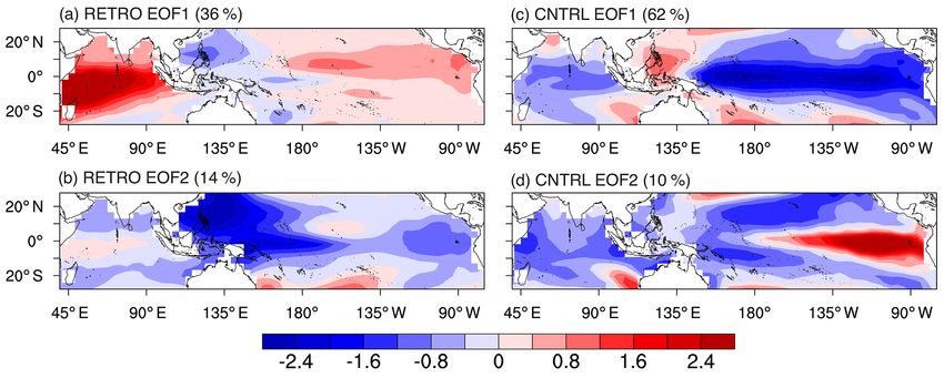
U. Mikolajewicz et al.: RETRO                                                                                                   1193

   The global ocean conveyer belt (Broecker, 1991), with             Earth’s rotation using a full Earth system model (ESM) run
meridional overturning in the North Atlantic fueling a deep          long enough to reach a stationary state, and wherein most
western boundary current that winds through the southern             components in the Earth’s oceans and biosphere (terrestrial
ocean, around Africa and into the Indian Ocean and North             land surface) were allowed to freely adapt to the changing
Pacific where waters again upwell, is a profound example of          conditions, and thereby define a new climate. Now, 200 years
a hemispheric asymmetry that might ultimately result from            after Humboldt first introduced the idea of showing climatic
zonal asymmetries in the climate system. The drivers of the          data on a map, and a century after Köppen perfected this tra-
conveyor belt are still inadequately understood. Though it           dition, we ask how different would his and subsequent maps
is clear that the salt advection feedback suggested by Stom-         have looked had the Earth rotated in the opposite direction.
mel (1961) stabilizes the current mode of overturning, it also       In addition to shining a light on some of the aforementioned
creates the potential for arresting the Atlantic overturning,        questions, these types of experiments provide important out-
which thus implies multiple equilibria of the thermohaline           of-sample tests of comprehensive climate models, the results
circulation. But why is deep water not formed in the North           of which, if reproduced by other groups, help shape the un-
Pacific? Two main mechanisms have been proposed (War-                derstanding of what aspects of Earth’s simulated circulation
ren, 1983), both invoking the role of zonal asymmetries. One         systems are less sensitive to the details of how the simulation
is that the net freshwater gain in the Pacific (and the corre-       system is constructed.
sponding net freshwater loss in the Atlantic) leads to saltier
subpolar water in the Atlantic and rather fresh water in the
subpolar North Pacific, thus stabilizing the fresh Pacific rel-      2   Model and experiments
ative to the salty Atlantic (Broecker, 1997). Another idea is
that the limited northward extension of the Pacific limits the       All simulations were performed with the ESM of the Max
cooling in the northernmost parts of the Pacific basin. In con-      Planck Institute for Meteorology (MPI-ESM, version 1.2;
trast, the Atlantic extends all the way into the Arctic allowing     Mauritsen et al., 2018), as developed for use in the Cou-
the surface water to be cooled down to the freezing point.           pled Model Intercomparison Project 6 (CMIP6; Eyring et al.,
   For many of the above questions, changing the direction           2016). The model contains the atmospheric general circula-
of rotation of the Earth thus presents an easy way to ob-            tion model ECHAM 6.3.02. This version contains some bug
tain a completely different climate, while maintaining the           fixes and a different tuning but is not structurally very differ-
familiar configuration of the continents and oceans. In the          ent from the version used in CMIP5 (Stevens et al., 2013).
new climate, changes in wind direction lead to changes in            The land component JSBACH 3.10 (Reick et al., 2013) in-
ocean circulation, precipitation patterns, and storm track lo-       cludes a dynamic vegetation model. Marine components are
cations in ways that inform our understanding of hemispheric         the general circulation Max Planck Institute ocean model
and longitudinal asymmetries of the present climate system,          (MPIOM 1.6.2p3; Jungclaus et al., 2013) and the marine bio-
such as the position of the tropical rain bands, or structure        geochemistry HAMburg Ocean Carbon Cycle (HAMOCC)
of the storm tracks. Two studies (Smith et al., 2008; Kam-           model (Ilyina et al., 2013; Paulsen et al., 2017). The coarse-
phuis et al., 2011) have explored the consequences of a ret-         resolution (CR) configuration of MPI-ESM is used. It con-
rograde rotation of the Earth with ocean circulation ques-           sists of ECHAM6 run with a T31 spectral truncation and
tions in mind. But even for these more-limited-in-scope stud-        with 31 vertical hybrid (sigma-pressure coordinate) levels
ies, the authors come to quite different findings. Smith et al.      reaching up to 10 hPa. In physical space, the spectral trans-
(2008) found an inverse conveyor belt circulation with strong        form grid on which parameterized processes are solved cor-
deep water formation in the North Pacific in a simulation            responds to 96 by 48 horizontal grid cells on a Gaussian
with the climate model FAMOUS (Smith, 2012). Using an-               grid. MPIOM has a curvilinear grid, with the poles located
other model, Kamphuis et al. (2011), meanwhile, found that           on Greenland and Antarctica. It has 120 by 101 grid cells
deep water formation in the North Atlantic weakened in their         in the horizontal and 40 levels in the vertical. A dynamic–
simulations, and intensified intermediate water formation be-        thermodynamic sea-ice model is included in MPIOM (Notz
came evident in the North Pacific. This study did not, how-          et al., 2013). The atmosphere and ocean are coupled once a
ever, show evidence of a complete reversal in the role of the        day.
subpolar North Atlantic and Pacific for deep water forma-               The forcing applied is the same as for the CMIP5 pre-
tion, leading to the conclusion that an altered net freshwater       industrial control run (Giorgetta et al., 2013) and corre-
flux is not sufficient to obtain the reversal, but that the conti-   sponds to 1850 climate conditions (fixed greenhouse gas con-
nental geometry is crucial for the pattern of the overturning        ditions, insolation, aerosols, ozone). All simulations were
circulation.                                                         started from an equilibrated climate state, resulting from a
   The two aforementioned studies, as noted, focus on the            long 8000-year spin-up with some minor changes in the ma-
effect of the direction of the Earth’s rotation on dynamics          rine biogeochemistry module during the run. The control run
with a focus on the ocean circulation. We are aware of no            (CNTRL) is simply a continuation of the spin-up and rep-
study that has simulated the effect of changing the sense of         resents Earth’s pre-industrial state. In the RETRO experi-

www.earth-syst-dynam.net/9/1191/2018/                                                  Earth Syst. Dynam., 9, 1191–1215, 2018
1194                                                                                              U. Mikolajewicz et al.: RETRO

ment, representing the retrograde rotating Earth, the sign of
the Coriolis parameter was changed both in the atmospheric
and oceanic model components. Additionally, the direction
of the Sun’s diurnal march was also reversed in the calcula-
tions of radiative transfer, thereby making sunrise consistent
with the sense of the planetary rotations. Each simulation
was integrated for 6990 model years. Whereas most physi-
cal variables were already reasonably well equilibrated after
2000 years (Fig. 1a), it took much longer for biogeochemical
tracers to come close to equilibrium (Fig. 1b). Some slight
drift in some water column inventories does however remain,
due to the interactive sediment processes whose timescales
are many millennia.
   Despite the ambition to simulate the Earth system in
a comprehensive manner, in a few aspects, the imprint
of Earth’s present-day climate was prescribed. Ice sheets,
greenhouse gases, and aerosols were prescribed according
to their present-day extent and pre-industrial concentrations,    Figure 1. Time series (100-year means) of meridional overturn-
respectively. The aerosol prescription means that dust depo-      ing circulation for the Atlantic (orange) and Pacific (turquoise) at
sition data used to run the ocean biogeochemistry model re-       30◦ N (a); a water mass tracer (PO∗4 ) at two locations in the north-
flect present-day estimates. Soil color and type were left un-    ern Atlantic (mean of 28–38◦ N, 60–70◦ W) and northern Pacific
changed in the land surface module JSBACH. The anthro-            (mean of 28–38◦ N, 150–160◦ W) (b). RETRO is shown by the
                                                                  solid lines and CNTRL by the dashed lines in both panels. PO∗4
pogenic land use was prescribed according to 1850 condi-
                                                                  (PO4 + O2 /172 − 1.5) combines concentrations of phosphate and
tions. These shortcomings in the model/experimental setup
                                                                  oxygen in such a way that, to first order, biological impacts are
will be dealt with in future experiments.                         eliminated and thus can be used as a (quasi-)conservative prop-
   The experimental setup was oriented on pre-industrial (pi-     erty, which in the prograde world is used to track the contributions
Control) conditions, as this run served as spin-up for CN-        of North Atlantic deep water (NADW) and Antarctic bottom wa-
TRL. Whereas the relative complete (with respect to the           ter (AABW) to the ventilation of the deep Pacific and Indian Ocean
components) ESM was run long enough to reach equilibrium          (Rae and Broecker, 2018).
for the climate, some biogeochemical components revealed
somewhat longer timescales as discussed above. Hence, for
the analyses, the last 1000 years of each experiment were         Labrador are free of sea ice in winter. Similar changes are
used. An exception is for the analysis of the atmospheric         evident in both the Aleutian Basin of the North Pacific and
short-term variability, which requires 2-hourly model out-        in the Pacific basin of the Southern Ocean. These changes
put and is based on the last 100 years of the experiments for     are also evident in the tropical sea surface temperatures, with
which high temporal resolution output was retained.               the region of warmest temperatures broadening to the east in
                                                                  RETRO as compared to a westward broadening in CNTRL
                                                                  (Fig. 2).
3   The atmosphere, its energy budget, and the                       Over the continents, the shifting isotherms mean that the
    surface climate                                               eastern continental margins warm and the western lands cool
                                                                  in RETRO as compared to CNTRL. In the midlatitudes, these
At a first glance, changing the sense of planetary rotation in-   changes are skewed (reflecting the changing inclination of
curs changes that Humboldt, or even Hadley (1735), might          Humboldt’s isotherms) so that the cooling in the western
well have anticipated. The patterns of surface winds and the      lands is amplified poleward, and the warming is strength-
polarity of the temperature distribution, or the inclination of   ened toward the Equator. Strong warming, for instance, is
the isotherms, is reversed (Fig. 2). The changes in the winds     evident in the southeast of Brazil (Rio de Janeiro), over the
are self evident, as the trades blow from the west in RETRO       southeastern states (Atlanta) of the US, and over southeast-
and the midlatitudes have surface easterlies. The change in       ern China (Guangzhou and the Pearl River Delta region). The
the inclination of the isotherms is perhaps most evident in       strongest cooling is over the ocean, in association with winter
the distribution of the sea-ice extent; this is shown by the      sea ice, particularly over the North and Baltic seas, although
faint blue lines in Fig. 2a and b, as well as the sea-ice dis-    west Africa, which is very warm in CNTRL, also cools sub-
tributions themselves presented in Fig. 3. In RETRO, win-         stantially, as does British Columbia in present-day Canada.
ter sea ice extends southward, enveloping Great Britain and       The magnitude of these changes have the effect that – from a
reaching as far south as the Bay of Biscay in the northeast At-   temperature perspective – the African–European landmasses
lantic, whereas the Canadian province of Newfoundland and         cool, and the Americas warm (Fig. 2c). Over the ocean, the

Earth Syst. Dynam., 9, 1191–1215, 2018                                                www.earth-syst-dynam.net/9/1191/2018/
U. Mikolajewicz et al.: RETRO 1195 Figure 2. Annual averaged surface temperature in RETRO (a), CNTRL (b), and the difference between both simulations (c). The light blue lines indicate the locations of 1 and 11 months of sea-ice coverage; annual precipitation in RETRO (d), CNTRL (e), and the difference between the two simulations (f). The curly vectors depict the annually averaged 10 m wind. The seasonal cycle is shown in videos in https://doi.org/10.5446/36560, https://doi.org/10.5446/36556, https://doi.org/10.5446/36557, https://doi.org/10.5446/36559 and https://doi. org/10.5446/36555. cold upwelling waters evident in the present-day east equato- tation; Fig. 2). The simulated warming of the southeastern rial Pacific largely vanish, rather than shift, in RETRO. Fig- regions of the continents coincides with marked drying, as ure 2 shows only a hint of a cold tongue stretching eastward precipitation is displaced to areas of present-day deserts in from east Africa in the equatorial Indian Ocean. RETRO (Fig. 2d and e). As was the case for temperature, To a large extent, the temperature changes also reflect some extracontinental-scale changes are evident as again the changes in patterns of precipitation. Circulation changes, un- roles of the Americas and the African–European land masses derlying changes in the inclination of the isotherms, are ev- are exchanged. The latter becomes substantially wetter as a ident in changes in the isohyets (lines of constant precipi- whole, particularly over Africa and the Mediterranean, and www.earth-syst-dynam.net/9/1191/2018/ Earth Syst. Dynam., 9, 1191–1215, 2018
1196                                                                                                      U. Mikolajewicz et al.: RETRO

Figure 3. Duration of sea-ice cover in RETRO (a, c) and CNTRL (b, d). The vectors show annual mean sea-ice transport. For technical
reasons, no sea-ice transport is displayed near the North Pole. The seasonal cycle of sea-ice coverage is shown in a video in https://doi.org/
10.5446/36557.

the former substantially drier (Fig. 2f). Precipitation in the           precipitation in RETRO results in a more tripolar, rather than
tropics shifts from the western oceans, where it is stronger             monopolar, tropical precipitation pattern, with distinct cen-
north of the Equator, particularly in the Pacific, to the east-          ters of precipitation over the Middle East, extending into
ern oceans and then south of the Equator, as in the Atlantic.            north Africa, over the southeast Atlantic, and into the central
This results in the zonally averaged precipitation becoming              Pacific. These changes are reflected in the 200 hPa velocity
slightly stronger south of the Equator, a point that we rejoin           potential (not shown), which becomes seasonally more vary-
below.                                                                   ing and less monopolar in RETRO as compared to CNTRL.
   RETRO also exhibits substantial changes in its monsoons                  To assess changing extratropical precipitation patterns, we
and deserts, something that might have been anticipated                  have also tracked individual extratropical cyclones, defined
based on earlier work by, e.g., Rodwell and Hoskins (1996).              as local minima of mean sea level pressure, in both RETRO
Whereas in CNTRL tropical precipitation, and the veloc-                  and CNTRL. The track densities obtained during DJF in the
ity potential (at 200 hPa) to which it is related, is strongly           Northern Hemisphere are presented in Fig. 4. Additional re-
focused around the western Pacific warm pool and Asian–                  sults for the tracking of cyclones during JJA in the South-
Australian monsoon complex, in RETRO there is a greater                  ern Hemisphere are shown in Fig. E2. As expected given
dislocation between the land and ocean influenced precip-                the changed sense of the zonal winds, the storms track west-
itation. Over Asia, the monsoon is displaced westward in                 ward rather than eastward in the midlatitudes. This analysis
RETRO, centering over the Arabian Peninsula. Atmospheric                 (Fig. E1) shows that changes in their characteristics (such
convection over the oceans, meanwhile, follows the warm                  as number, lifetime, growth rate, or intensity) are small, al-
waters to the east in RETRO, and becomes more prevalent                  though a tendency for slightly (2 hPa) more intense storms
over the central and eastern Pacific and the southeastern At-            in RETRO is evident. This may be related to strengthen-
lantic. The area with the largest amount of annual precipi-              ing meridional temperature gradients, as discussed near the
tation is located near Ascension Island in the southern trop-            end of this section. The tracks of storms, however, change
ical Atlantic (8◦ S, 14◦ W), which takes on a climate more               more substantially as they move from regions of the western-
like present-day Palau (8◦ N, 134◦ E). Overall, the disloca-             boundary currents in CNTRL to become more land cen-
tion between oceanic (warm-pool) and terrestrial (monsoon)               tered (RETRO) in the Northern Hemisphere, with particu-

Earth Syst. Dynam., 9, 1191–1215, 2018                                                       www.earth-syst-dynam.net/9/1191/2018/
U. Mikolajewicz et al.: RETRO                                                                                                              1197

                      RETRO                                       CNTRL                                    RETRO-CNTRL

               5     10      15     20     25      30     35    40     45      50          32    24   16    8     0    8   16   24    32
                                         Tracks density                                                     Difference

Figure 4. Track density (number of tracks per season for a unit area equivalent to a 5◦ spherical cup) computed for the Northern Hemisphere
during the December–January–February (DJF) season. The tracking is performed using 2-hourly mean sea level pressure (MSLP) data;
storms are defined as local minimum of MSLP and are tracked during their lifetime using the methodology described in Hoskins and Hodges
(2002). The data are seasonally averaged over the last 100 years of each simulation. In the first two plots on the left track, density for RETRO
and CNTRL is shown; values below 5 are masked for the sake of visualization. Shown in the rightmost plot is the difference between RETRO
and the CNTRL simulation without any masking applied. For the Southern Hemisphere version of this figure, see Fig. E2.

larly strong storm activity extending from the Caspian Sea                  wetter climate over the Sahara. This is shown in Appendix B,
and Arabian Sea through the northern Mediterranean (see                     and confirms that major circulation changes seen in RETRO
videos in https://doi.org/10.5446/36561 and https://doi.org/                versus CNTRL are ultimately dynamically driven through
10.5446/36555). This has large implications for the climate                 changes in the sign of Earth’s absolute angular momentum.
of north Africa and the Middle East but also acts to freshen                   Despite large regional shifts in circulation patterns, the
the Atlantic at the expense of the Indo-Pacific oceans, with                globally averaged energy budget of RETRO hardly differs
implications for the meridional overturning circulation (see                from that of CNTRL, and those differences that do emerge
Sect. 5). Further to the west, storms are most pronounced                   tend to be smaller than our ability to match the energy budget
along the northern boundary of the Great Lakes (Fig. 4), east               as derived from observations (Stevens and Schwartz, 2012;
of the continental divide.                                                  Stephens et al., 2012). Figure 6 is adapted from Stevens and
   Changes in the storm tracks and trade winds lead to sig-                 Schwartz (2012) and shows that RETRO is slightly cooler
nificant changes in the atmospheric energy transport, specif-               (by about 0.14 ◦ C, with less upwelling terrestrial radiation
ically in the moist static energy transport as shown in Fig. 5.             from the surface; see Table 1), cloudier, and wetter. The in-
Large amounts of moist static energy are transported from                   crease in cloudiness is evident in a slight increase in plan-
the Atlantic towards north Africa and the Middle East, where                etary albedo, with an additional 1 W m−2 of reflected solar
they have large implications for the regional climate. This                 radiation. Surface turbulent moisture fluxes are larger and
transport persists through all seasons, except winter, when                 sensible heat fluxes are smaller in RETRO. These changes
the trade winds are deflected southward across Nigeria to-                  are consistent with more terrestrial radiation to the surface,
wards equatorial Africa (not shown) extending into the In-                  indicative of an atmosphere that cools and hence rains more.
dian Ocean. Further, moisture is transported from the Indian                The surface cooling in RETRO is manifested entirely in the
Ocean across India, Pakistan, and the Middle East towards                   Northern Hemisphere, as the Southern Hemisphere actually
the Mediterranean Sea during all seasons except fall (Fig. 5).              warms by 0.28 ◦ C. In RETRO, the difference between the av-
The enhanced moisture flux towards north Africa and the                     erage temperature of the Northern Hemisphere and Southern
Middle East from the Atlantic and Indian Ocean provides a                   Hemisphere is −0.40 ◦ C, as compared to +0.57 ◦ C in CN-
proximate explanation for the significant greening in these                 TRL. Concomitantly, almost all of the change in the down-
areas (Sect. 4). It also indicates a strong interplay between               ward longwave feedback (5.7 W m−2 ) is in the Northern
the trade winds over the Atlantic and the storm track over the              Hemisphere, and almost all of this is over land.
Middle East.                                                                   Changes in the mean energy budget could be expected to
   Changing the direction of the diurnal path of the Sun has                affect the zonal distribution of precipitation. Building on the
only minor influence on the climate but contributes to a                    ideas developed by Kang et al. (2008, 2009) and Frierson
southward shift of the ITCZ over the tropical Atlantic and a                et al. (2013), Bischoff and Schneider (2014) argue that an in-

www.earth-syst-dynam.net/9/1191/2018/                                                           Earth Syst. Dynam., 9, 1191–1215, 2018
1198 U. Mikolajewicz et al.: RETRO
Table 1. Changes in precipitation and surface temperature. For
these entries, the tropics are defined as between 22.3◦ S and
22.3◦ N.
Global NH SH Tropics
Surface temperature (K)
RETRO 287.42 287.21 287.64 298.98
CNTRL 287.56 287.76 287.36 298.53
Precipitation (mm day−1 )
RETRO 3.11 3.18 3.05 4.09
CNTRL 3.04 3.04 3.04 4.05
spheric asymmetries in the distributions (as opposed to the
shape) of continents (i.e., the fact that Antarctica is in the
Southern Hemisphere) are at least not sufficient to explain
why the ITCZ is mostly north of the Equator.
Many of the points discussed above are amplified by an
inspection of the latitude–height description of the zonally
averaged circulation. Figure 8a shows the differences be-
tween RETRO and CNTRL of annually and zonally averaged
temperatures. Figure 8b presents the corresponding annually
and zonally averaged zonal winds. The surface temperature
Figure 5. Moist static energy transport for RETRO (a) and CN- anomaly pattern shows the tropical warming in RETRO and
TRL (b). To calculate the transport, we use 2-hourly data of veloc-
the strong northern hemispheric cooling. The subtropical jets
ities, surface pressure, temperature, and specific humidity (Keith,
in RETRO are shifted northwards, i.e., equatorwards in the
1995). The data are averaged over the last 100 years of the simula-
tion. SH and polewards in the NH, and slightly increased in mag-
nitude. This is consistent (through the thermal wind balance)
with changes in tropospheric temperatures whereby the high-
latitude cooling in RETRO is much more pronounced in the
crease of energy release into the tropical atmosphere would Northern Hemisphere. This pattern of tropical warming and
shift the zero crossing of the vertically and zonally aver- high-latitude cooling implies greater baroclinicity at midlat-
aged moist static energy transport (the energy flux Equator) itudes but is accompanied by relatively little change in storm
equatorward. Likewise, this way of thinking suggests that the activity (see above), suggesting that enhanced northern hemi-
strong increase in the RETRO Northern Hemisphere merid- spheric energy fluxes are mostly attributable to the changing
ional temperature gradients implies a strengthening of the enthalpy gradients.
northern hemispheric energy fluxes which should also be ac- As typical for climate model simulations of global warm-
companied by a southward shift of the ITCZ. Such a shift in ing, the tropical warming is stronger in the free troposphere
the ITCZ is indeed pronounced in the simulations (Fig. 7a). than at the surface and reaches about 1.7 K around 300 hPa.
The shift is also predicted by the change in the energy budget Also typical for a globally warmer tropical troposphere is the
Equator (Fig. 7b, and inset), although not by the magnitude increase of the cold-point tropical tropopause, i.e., the cold-
of the shift, nor does its position correlate well with the actual est point in the tropical tropopause region, as one might also
position of the precipitation maximum. These discrepancies expect if the tropopause temperature is radiatively controlled
might be related to changes in the zonally asymmetric circu- following the ideas of Zelinka and Hartmann (2010), which
lation as earlier argued by Wallace et al. (1989) and Philan- in RETRO is about 0.6 K warmer than in CNTRL.
der et al. (1996). To the extent the changes in precipitation A warmer cold-point tropopause and the resulting in-
are consequences of the changed hemispheric energy bud- creased water vapor entry into the stratosphere is the likely
get, they point to a possible role for ocean circulation and cause of an about 13 % larger specific humidity in the lower
its disproportionate impact on the northern hemispheric ice to middle stratosphere in RETRO (not shown). More strato-
sheets and temperature gradients, particularly over the North spheric water vapor is a plausible reason for the, in general,
Atlantic. Reversing the sense of the planetary rotation does lower stratospheric temperatures.
not, however, affect the distribution of land masses, so that Changing the planetary rotation should, of course, to a
differences between RETRO and CNTRL suggest that hemi- first order cause a reversal of zonal winds. Figure 8b shows
Earth Syst. Dynam., 9, 1191–1215, 2018 www.earth-syst-dynam.net/9/1191/2018/U. Mikolajewicz et al.: RETRO 1199
Figure 6. Globally averaged energy budget contributions for RETRO and CNTRL.
hemispheric baroclinicity, and is related to a stronger po-
lar vortex in RETRO. The average eddy heat flux entering
the stratosphere in boreal winter between 40 and 80◦ N is
weaker in RETRO by about 15 % (not shown), thereby help-
ing to explain the temperature changes required to balance
this stronger polar vortex. The changes in tropospheric flow
patterns are thus connected to the stratosphere. The latitude
dependence of the temperature signal in the southern strato-
sphere, although consistent with changes in vertical motion,
is less straightforward to interpret.
In two sensitivity experiments (abrupt quadrupling of at-
mospheric CO2 , CNTRLx4, and RETROx4), the climate
sensitivity was investigated. Details are given in Appendix C.
In general, RETROx4 showed a higher climate sensitivity
(approximately 10 % to 15 %). In spite of the large differ-
ences in tropical climate, the strength of the tropical cloud
effect seems to be rather similar between the prograde and
the retrograde simulations. A striking difference appears in
the long-term equilibration (years 1000–2500), where CN-
TRLx4 shows a change towards much faster equilibration at
a lower level which is absent in RETROx4. This difference is
connected to differences in the heat uptake of the deep ocean.
Figure 7. Zonally and annually averaged (a) precipitation, and
(b) atmospheric energy flux for RETRO (black, solid) and CNTRL 4 Land surface and biosphere
(red, dashed). The inset in panel (b) shows the atmospheric energy
flux (computed as the integral of the vertical heat flux convergence Köppen, in his book Die Klimate der Erde (1923), outlined
as a function of latitude) in the vicinity of the zero crossing near the his ideas regarding how continents impart zonal asymmetries
Equator. in climate using his classification system applied to an ide-
alized continent. For the purposes of the present discussion,
Köppen’s idealized continent has been redrafted and is pre-
the sum of annually and zonally averaged zonal winds of sented in Fig. 9. The expectation inherent in this idealization
RETRO and CNTRL, which indicates second-order effects, is that a retrograde rotating Earth would experience mirror
i.e., deviations from a simple change in sign. Changes in the symmetry about the north–south axis in its climate zones.
stratospheric circulation should be interpreted with caution As might have been expected given the discussion of the
due to the model top in the middle stratosphere at 10 hPa. previous section, predictions based on Köppen’s idealized
However, the strongest stratospheric cooling, which occurs continent, both for the distribution of climate zones in the
in the polar Northern Hemisphere, is dominated by a cool- present-day climate, and for the expected mirror symmetry
ing in boreal winter, which further contributes to northern for a retrograde rotating Earth are well supported by CN-
www.earth-syst-dynam.net/9/1191/2018/ Earth Syst. Dynam., 9, 1191–1215, 20181200 U. Mikolajewicz et al.: RETRO
Figure 8. (a) Annually and zonally averaged temperature difference between RETRO and CNTRL (left) and its tropical (20◦ S to 20◦ N)
average (right). The tropopause level indicated in the right panel refers to the cold-point tropopause of the control case. (b) Annually and
zonally averaged zonal wind sum of RETRO and CNTRL. White contour lines show the isotherms and isotachs of the control simulation
with a contour interval of (a) 10 K and (b) 10 m s−1 .
RETRO CNTRL Table 2. Global area of main vegetation groups averaged over the
last 1000 years of the experiment.
North Pole North Pole
Area covered (million km2 ) RETRO CNTRL Difference
60° N 60° N 60° N
Permanent deserts
30° N 30° N 30° N
Global 31.2 41.8 −10.6
0° 0° 0° NH 21.0 34.1 −13.1
SH 10.2 7.7 +2.5
30° S 30° S 30° S
Woody vegetation
60° S 60° S 60° S
Global 46.3 41.3 +5.0
NH 33.4 25.0 +8.4
South Pole South Pole
SH 12.9 16.3 −3.4
Af Aw BS BW Cf Cs Cw Df Dw ET EF
Herbaceous vegetation
Figure 9. Classification of climate zones for an idealized continent, Global 50.0 44.4 +5.6
the Klimarübe, following Köppen (1923). First letters in the leg- NH 41.1 36.4 +4.7
end are main climate types: A: equatorial, B: arid, C: warm temper- SH 9.0 8.0 +1.0
ate, D: snow, and E: polar. Second letters are precipitation regimes:
W: desert, S: steppe, f: fully humid, s: summer dry, w: winter dry,
T: tundra, and F: ice cap.
first approximation in a retrograde rotating Earth, these fea-
tures do appear with mirror symmetry (Fig. 10b).
There are however some differences that would not have
TRL and RETRO. This is shown, using the same indica- been predicted from just mirroring the idealized continent.
tion of major climate zones, in Fig. 10. CNTRL reproduces Most prominent is the shift in deserts from the Eurasian–
both the north–south asymmetry associated with more north- African continental mass to the Americas, with a greater cen-
ern hemispheric land masses as reflected by the emergence ter of mass over the subtropical southern hemispheric con-
of cold winter climates (Dw and Df) in the Northern Hemi- tinents. This change is consistent with the inferences of the
sphere, and the east–west asymmetry of a variety of features. last section, whereby in RETRO many of the climate features
For instance, the shift from subtropical deserts (BW) in the associated with present-day Europe/Africa and North/South
continental southwest toward moist temperate climates in the America are exchanged.
continental southwest at subtropical latitudes is well evident
in the contrast between west Africa and southeast Asia. To a
Earth Syst. Dynam., 9, 1191–1215, 2018 www.earth-syst-dynam.net/9/1191/2018/U. Mikolajewicz et al.: RETRO 1201
(a) (a) RETRO
(b)
(b) CNTRL
Figure 10. The 11 main climate zones after the Köppen–Geiger
classification (colors) for (a) RETRO and (b) CNTRL. First let-
ters in the legend are main climate types: A: equatorial, B: arid, 20 % [m² m-²]
Tree 50 %
C: warm temperate, D: snow, and E: polar. Second letters are pre- cover
80 % 0.5 1 2 3 4 5 6
cipitation regimes: W: desert, S: steppe, f: fully humid, s: summer
dry, w: winter dry, T: tundra, and F: ice cap.
(c) RETRO - CNTRL
The complete replacement of the wide desert belt from
west Africa to the Middle East by forests and humid grass-
lands is more quantitatively measured by changes to the leaf
area index (LAI; Fig. 11). Changes in LAI also illustrate the
degree to which the retreat of desert climates in Africa and
Eurasia is accompanied by an extensive formation of dry cli-
mates in South and North America. Southern Brazil and Ar-
gentina become the Earth’s biggest deserts and the southern
states of the United States see a dramatic climate shift from a
fully humid climate towards a complete aridification. In gen-
eral, many dry regions are simulated in RETRO, but extreme [m² m-²]
deserts – like the present-day Sahara – are less widespread.
-5 -3 -1 0 1 3 5
Changes are, as discussed in Sect. 3, consistent with circula- -
tion and precipitation changes over these same regions. Figure 11. LAI (shaded) and tree cover (contours) for (a) RETRO
The global area covered by permanent deserts is reduced and (b) CNTRL. Panel (c) shows the differences in LAI (see also
by about 25 % from 42 × 106 and 31 × 106 km2 (see Ta- video in https://doi.org/10.5446/36553).
ble 2). Woody and herbaceous vegetation fills the new vege-
tated areas in about equal measure. The greening is concen-
trated over northern hemispheric land masses (desert areas tree-covered area is reduced by about 20 %. Tropical veg-
shrink by nearly 40 %) and mostly attributed to the afore- etation remains largely unaffected in Africa and Asia. In
mentioned vanishing of the wide desert belt from west Africa South America, the Amazon rain forest shrinks substantially,
to the Arabian Peninsula. Over southern hemispheric land though.
masses, deserts and grasslands spread slightly, whereas the
www.earth-syst-dynam.net/9/1191/2018/ Earth Syst. Dynam., 9, 1191–1215, 20181202 U. Mikolajewicz et al.: RETRO
The greener climate in RETRO affects the global carbon
storage on land, which increases by 86 Pg C compared to
the CNTRL simulation. The globally integrated storage in-
crease is composed of an increase by 215 Pg C in the North-
ern Hemisphere and a decrease of 130 Pg C in the Southern
Hemisphere.
Based on previous experience (e.g. Claussen, 2009; Bathi-
any et al., 2010), we suppose that interactions between the
biosphere and the atmosphere amplify or dampen the near-
surface climate changes. The reduced tree cover in the much
colder and snowier Europe, for example, coupled with the
greening of north Africa and the Middle East likely in-
duces a large-scale and large-amplitude change to the sur-
face albedo (Fig. 12). These changes are expected to mod-
ify the local climate directly, for instance, through enhanced
near-surface cooling via the effect of reduced snow mask-
ing, or indirectly by inducing circulation changes. The de- Figure 12. Differences in surface albedo (RETRO–CNTRL).
picted changes in surface albedo (Fig. 12) also hint at a lim-
itation of our study. We have prescribed present soil albedo
and land use as of 1850 CE. Hence, we expect that changes of ters on the western side of the basins leads to a local cooling
soil albedo caused by an increase in soil carbon due to plants (Fig. 2a and c).
growing in the retrograde green Sahara (see Vamborg et al., The Antarctic circumpolar current (ACC) reverses its di-
2011) could further decrease the surface albedo in that region rection and moves from east to west in RETRO. The In-
or, vice versa, enhance the surface albedo in the retrograde donesian throughflow changes it sign and transports 21 Sv
deserts of the Americas. Likewise, the atmospheric aerosol from the Indian Ocean to the Pacific. Besides, many of the
remained unchanged in the simulations, with an interactive gyres show substantial changes in strength. In RETRO, both
aerosol, precipitation changes over RETRO in Africa, and subtropical and subpolar gyres in the North Atlantic become
hence Sahara dust emissions would likely decrease; whether weaker than in CNTRL. The main cause for this is the lack
this would be compensated by substantial increases in emis- of the thermohaline-driven overturning component in the At-
sions from other sources remains an open question. lantic (see below), reducing the North Atlantic gyres to their
Another prescribed present-day feature is the ice sheets. wind-driven part. Further, the straight western coastline of
In the RETRO and CNTRL simulations, no permanent snow the Americas enables the development of closed gyres in the
cover was simulated outside of the prescribed glaciated ar- Pacific in RETRO. In contrast, the gyres in CNTRL are af-
eas (not shown). Additionally, the simulated summer tem- fected by the openings along the highly structured Asian–
peratures over the ice sheets (not shown) do not indicate a Australian coastline. Especially the South Pacific subtropical
strong inconsistency between the prescribed ice sheets and gyre in RETRO becomes (with more than 130 Sv) approxi-
the simulated climate both for RETRO and CNTRL. There- mately 2.5 times stronger than in CNTRL.
fore, we did not find a major inconsistency between the pre- In CNTRL, Antarctic bottom water is formed in the cen-
scribed present-day ice sheet configuration and the simulated ter of the Weddell Gyre. In RETRO, deep water formation
climate. in the Southern Hemisphere (as indicated by the maximum
mixed layer depth; Fig. 14) takes place in the Atlantic sec-
tor of the Southern Ocean, close to the coast of Antarctica.
5 Ocean physics In the Northern Hemisphere, the changes are more dramatic.
In CNTRL, the model simulates an Atlantic meridional over-
As expected, the change of the sign of the Coriolis parameter turning circulation (MOC) of 19 Sv. North Atlantic deep wa-
has a marked impact on the ocean circulation (Fig. 14; see ter is formed in the Nordic Seas and intermittently in the
video in https://doi.org/10.5446/36551). Directly associated Labrador Sea. In RETRO, only intermittent convection down
with this shift is a change in the sign of the zonal ocean ve- to 2000 m depth occurs in the North Atlantic (Fig. 14). The
locity components. Subpolar and subtropical gyres shift their appearance of deep convection has a multidecadal timescale
longitudinal positions and what used to be a western bound- with a peak around 80 years. In the long-term mean, no clear
ary current in CNTRL becomes an eastern boundary current North Atlantic deep water cell emerges in RETRO. Instead,
in RETRO. These shifts cause significant changes in the SST the northeast Pacific exhibits strong formation of deep wa-
patterns in the subtropical gyres. The strong poleward trans- ter (down to 3000 m). This leads to a strong Pacific MOC of
port of warm water in the eastern boundary currents leads to 23 Sv (Fig. 13). The core of the North Pacific deep water is
a local warming and the missing poleward flow of warm wa- slightly warmer and shallower than its North Atlantic equiv-
Earth Syst. Dynam., 9, 1191–1215, 2018 www.earth-syst-dynam.net/9/1191/2018/U. Mikolajewicz et al.: RETRO 1203
alent in CNTRL. This indicates that the Atlantic and Pacific Table 3. Global mean net primary production rate, biogenic
change their roles in CNTRL and RETRO. material export flux at 100 m, volume of oxygen minimum
Whereas the global poleward oceanic heat transport in the zones (OMZs), global mean denitrification, and ratio of denitrifi-
Northern Hemisphere is almost unchanged (1.56 PW in CN- cation to organic matter export flux on a percentage basis (Rden ).
TRL versus 1.52 PW in RETRO at 30◦ N; Fig. 15a), the dis-
tribution between the basins changes strongly. In CNTRL, Net primary production (Gt C yr−1 )
more than half of the heat is transported in the Atlantic. In Bulk phytoplankton Cyanobacteria Total
RETRO, the Pacific transports almost 80 % of the heat. The CNTRL 49.97 3.09 53.05
transport in the Pacific is larger, as the gyre transport in the RETRO 48.02 3.73 51.75
Pacific is stronger than in the Atlantic, which can be ex-
Export flux
plained by the larger spatial extent of the basin. Thus, also
in terms of the ocean heat transport, the Atlantic and Pa- Organic matter Opal shells Calcite shells
cific have changed their roles. Due to the strong upwelling (Gt C yr−1 ) (kmol Si s−1 ) (Gt C yr−1 )
of colder subsurface water, the tropical Indian Ocean (north CNTRL 7.58 3464.0 0.54
of 30◦ S) becomes a strong heat sink for the atmosphere in RETRO 7.78 3422.7 0.49
RETRO (0.84 PW). This is in contrast to CNTRL, where
Volume of OMZ Denitrification Rden
the tropical Indian Ocean has a rather small net heat uptake (1016 m3 ) (Tg N yr−1 ) (%)
(0.1 PW). In RETRO, the tropical Indian Ocean has de facto
taken the role of the tropical east Pacific in CNTRL. This CNTRL 3.90 109 1.07
RETRO 3.83 154 1.46
is also true for tropical SST variability. The leading mode
in RETRO has its center of action in the Indian Ocean, in
contrast to the El Niño mode in CNTRL. More details can
be found in Appendix A. For the export of heat to the tropi- tion (as in CNTRL). This has dramatic consequences for the
cal Pacific, the reversed Indonesian throughflow plays a key overturning circulation in these basins. Whereas both basins
role. In RETRO, the equivalent of the cold Humboldt Current today (and in CNTRL) are characterized by deep convection
flows northward in the western Indian Ocean along the coast and a deep outflow of salty water, the circulation in RETRO
of Mozambique. is completely reversed. Both basins are well stratified and the
The changes in ocean heat transport are also reflected in main source of deep water is the inflow. The outflow at the
SST and sea-ice changes. In general, the North Atlantic is surface is rather fresh, typical for estuarine circulations.
colder in RETRO, while the North Pacific is warmer (Fig. 2). The lack of deep water formation in the North Atlantic and
The effect of the reduced ocean heat transport in the North the Arctic and the changes in density lead to an increase in
Atlantic is amplified by the reduced wintertime mixed layer sea level in the Atlantic and the Arctic by typically 0.5 m,
depth, which reduces the effective heat capacity of the sur- whereas the sea level in the Pacific and the Indian Ocean
face ocean and thus leads to colder winter temperatures and decreases (not shown). This reverses the sea level gradient
extended sea-ice cover (Fig. 3). across Bering Strait and leads to a southward flow of fresh
In RETRO, the Atlantic north of 30◦ N is a strong sink Arctic surface waters into the North Pacific.
for atmospheric moisture (0.70 Sv), and the net flux into the The direction of the simulated changes is similar to the
North Pacific is much smaller (0.10 Sv), whereas in CNTRL outcome of experiments by Smith et al. (2008) and Kamphuis
these values are almost equal (Fig. 15b). The net moisture et al. (2011), but in general the circulation changes found
loss of the Pacific north of 30◦ S is 0.30 Sv; in the Atlantic, in our model are more similar to the results of Smith et al.
it is only 0.07 Sv. In CNTRL, the role of the two oceans (2008) than to the results of Kamphuis et al. (2011). Both
is reversed. In RETRO, the Atlantic gains moisture from studies showed a weakening of the Atlantic MOC together
the Indian Ocean by atmospheric moisture transport across with a surface freshening in the North Atlantic and saltier
the Middle East, which is strongest in spring and summer surface conditions in the North Pacific. Whereas Smith et al.
and loses moisture by the eastward transport across equa- (2008) also showed a strong MOC in the Pacific, Kamphuis
torial Africa. The transport across Central America is very et al. (2011) obtain a state with a relative weak MOC both in
small but directed towards the Atlantic, whereas in CNTRL the Atlantic and Pacific.
a strong transport is directed towards the Pacific (Fig. 5).
Consequently, the North Pacific surface salinity in RETRO is 6 Ocean biogeochemistry
higher than in CNTRL; in the North Atlantic, surface salinity
is reduced (see video in https://doi.org/10.5446/36558). This Ocean circulation is the key driver of spatial patterns of ma-
explains the shift of the deep water formation from the North rine biogeochemical tracers. This implies large-scale patterns
Atlantic to the North Pacific described above. of these tracers follow the reversal of the ocean circula-
Due to strong precipitation in RETRO, the Mediterranean tion (described in Sect. 5) and biogeochemical water mass
and Red Sea no longer are marginal seas with net evapora- trackers, such as PO∗4 , mirror the transient behavior of the
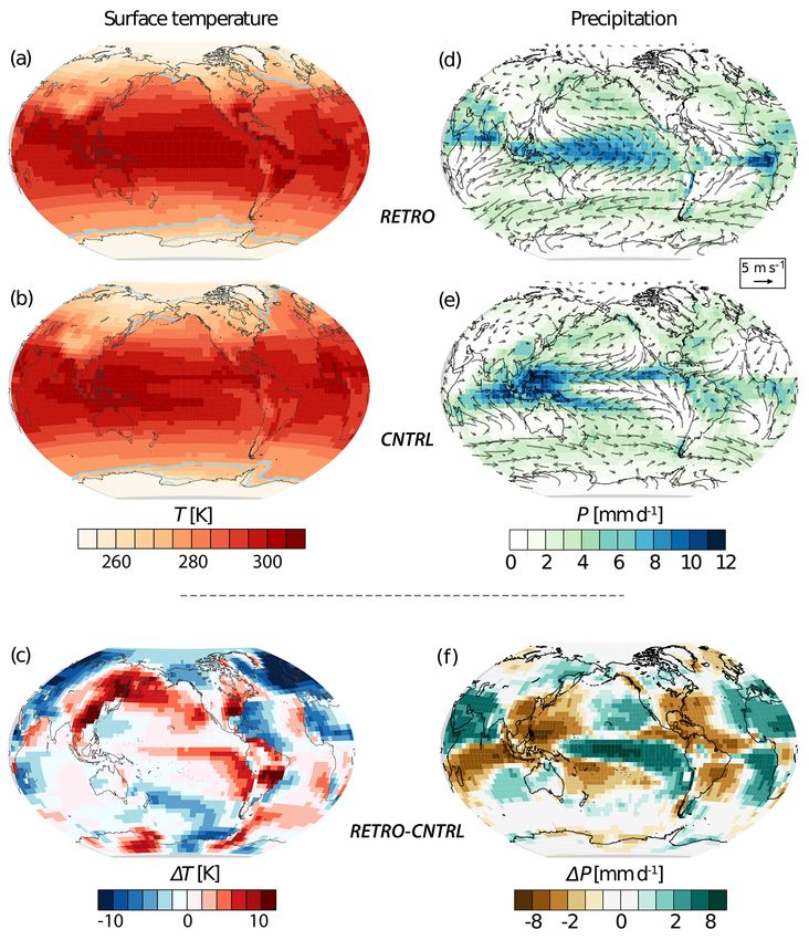
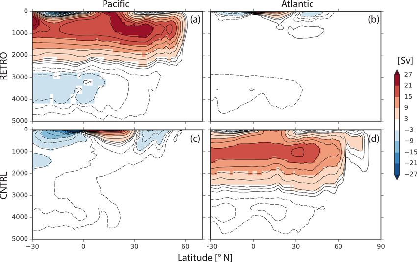
www.earth-syst-dynam.net/9/1191/2018/ Earth Syst. Dynam., 9, 1191–1215, 20181204 U. Mikolajewicz et al.: RETRO Figure 13. MOC stream functions. Outlines are at ±1, 2, and multiples of 3 Sv. The Indian Ocean MOC stream functions are shown in Fig. 17. Figure 14. Maximum mixed layer depths and annual mean barotropic stream functions. Outlines are at ±5, 10, 20, 60, 100 Sv, and so on. (a) RETRO, (b) CNTRL. MOC reversal though with longer equilibration timescales volume of these oxygen minimum zones (OMZs) is nearly (Fig. 1b). Planetary-scale features such as zonal and global identical in RETRO and CNTRL (Table 3; see also video means are largely unaffected by the direction of Earth’s ro- in https://doi.org/10.5446/36552). Despite that, in CNTRL, tation (Table 3). The changes in the Coriolis effect and wind three major OMZs are found on the eastern side of each patterns lead to a shift of eastern boundary upwelling systems ocean basin, while in RETRO there is one sizable OMZ in to the western sides of ocean basins in RETRO (Fig. 16). the Indian Ocean. Strong upwelling, which is also reflected in In these upwelling systems, in general, primary production, strong heat uptake, fuels biological production rates at levels and thus carbon storage in particulate organic matter (POM), not found in CNTRL. In combination with the circulation and is driven by a continuous supply of nutrients from greater the basin geometry of the Indian Ocean, this leads to very low depth into the sunlit surface layers (euphotic zone). Gravi- ventilation and nutrient accumulation in the northern part of tational settling and subsequent remineralization of POM, a the basin (Fig. 17) and results in the development of this ex- process being referred to as biological pump, lead to pro- tended OMZ. One prominent characteristic of OMZs is that nounced vertical gradients in all biogeochemical tracers. Ex- in the low oxygen environment denitrifying bacteria are able ported organic material is remineralized under the consump- to access food energy by degradation of organic matter using tion of oxygen. For this reason, hypo- or suboxic conditions nitrate (NO3 ). Denitrification is limited to very low oxygen are often found at intermediate depths in regions with high conditions (in the model O2 ≤ 0.5 mmol m−3 ) and is the only biological production such as upwelling systems. The global remineralization process that selectively removes bioavail- Earth Syst. Dynam., 9, 1191–1215, 2018 www.earth-syst-dynam.net/9/1191/2018/
U. Mikolajewicz et al.: RETRO                                                                                                   1205

                                                                          The model setup, of course, includes simplifications that
                                                                       might affect characteristics of the response. For example, due
                                                                       to lack of a dynamical aerosol model, we use dust deposition
                                                                       maps derived from a prograde model as a source of dissolved
                                                                       iron. Thereby, large ocean inputs occur downstream major
                                                                       deserts, such as from the Sahara into the Atlantic. A displace-
                                                                       ment of deserts as simulated by the land model in RETRO
                                                                       (see Sect. 4) would also imply a shift of dust deposition max-
                                                                       imums. This might affect the relative importance of P and
                                                                       iron limitation of cyanobacteria (as described in Sohm et al.,
                                                                       2011). Hence, the availability of dissolved iron in RETRO is
                                                                       controlled by ocean circulation patterns and upstream con-
                                                                       sumption by plankton in regions where local aeolian supply
                                                                       is low due to the fixed (prograde) dust deposition field. On
                                                                       the contrary, some regions like the northern Indian Ocean re-
                                                                       ceive potentially a higher iron supply by this dust field. How-
                                                                       ever, the dominance of cyanobacteria in the northern Indian
                                                                       Ocean in RETRO is primarily a result of the interplay be-
Figure 15. Northward implied ocean transport of (a) heat and
                                                                       tween the high equatorial primary production creating water
(b) freshwater. Black: global, orange: Atlantic, turquoise: Pacific,
and violet: Indian Ocean. Solid: RETRO, dashed: CNTRL.                 masses depleted in nitrate and enriched in phosphate and iron
                                                                       and the ocean circulation with a northward transport and sub-
                                                                       sequent upwelling of these water masses (Fig. D1). Indepen-
able nitrogen. All other degradation processes, i.e., aerobic          dent of aeolian iron supply, the lack of nitrate (Fig. 18) in-
remineralization and sulfate reduction, convert organic mate-          hibits growth of bulk phytoplankton fostering the local dom-
rial into phosphate, iron, and nitrate. In RETRO, global den-          inance of cyanobacteria in the northern Indian Ocean.
itrification is about 50 % higher than in CNTRL and takes                 Furthermore, atmospheric mixing ratios of CO2 are set to a
place predominately in the northern Indian Ocean (Table 3;             constant global value. A simulation with a fully coupled car-
see also video in https://doi.org/10.5446/36554). As a con-            bon cycle would have allowed for assessing local interactions
sequence, upwelling of nitrate-depleted and phosphate-rich             between land cover and subsequent CO2 emission changes
water (N∗ = NO3 − 16 · PO4 < 0; Fig. 18) results in a shift            driven, e.g., by the shifts in the Indian monsoon. However,
of the phytoplankton species composition (Fig. 17) with a              we expect that main features of ocean carbon cycling would
dominance of cyanobacteria in RETRO. Most phytoplank-                  remain unaffected.
ton species need both nitrate and phosphate for their growth.
Only cyanobacteria are able to grow on dinitrogen (N2 ),
as long as sufficient phosphate and iron are available (e.g.,          7   Conclusion
Sohm et al., 2011). In the prograde world, only few re-
gions exist where the surface water is nitrate-depleted and            By performing experiments, where the sense of rotation of
phosphate-rich. Thus, cyanobacteria are outcompeted nearly             the Earth was changed, we aimed at better understanding
everywhere by other phytoplankton species (bulk phyto-                 climate with respect to hemispheric asymmetries and lon-
plankton). In contrast, in RETRO, they become the dominant             gitudinal distributions. Two simulations, each encompassing
primary producer in the northern Indian Ocean. The change              6990 years forced by conditions thought to be representative
of the Earth’s rotation direction and the subsequent develop-          of Earth’s climate before the era of industrial combustion
ment of an extended oxygen minimum zone in RETRO pro-                  (i.e., 1850), are performed: one with a retrograde rotating
voke plankton species compositions over large areas which              Earth (RETRO) and the other being the control climate (CN-
have not been observed in the prograde world.                          TRL) of the prograde rotating Earth. The simulations, while
   It was hypothesized that a warming climate and the conse-           endeavoring to be as comprehensive as possible, are not with-
quential deoxygenation of the ocean (e.g., Breitbarth et al.,          out limitations. For instance, their resolution is coarse, so
2007; Hutchins and Fu, 2017) trigger such an ecosystem                 as to expedite the long equilibration of the ocean and bio-
shift with nitrogen-fixing cyanobacteria as a potential winner.        geochemical cycles, and some other constituents (ice sheets,
Thus, the response nicely supports the possibility of these            soil properties, greenhouse gases, aeolian dust input, and the
extreme changes in the ecosystem. It also demonstrates the             atmospheric aerosol) are held constant consistent with the
model’s ability to adapt to an unconventional forcing and to           present-day (or pre-industrial) prograde rotating Earth. These
simulate phenomena which are a result of complex interac-              simplifications could be relaxed in future studies. Even so,
tion of abiotic and biotic processes.                                  the simulations are the first of their kind as two previous
                                                                       studies looked in a much more limited way, and over shorter

www.earth-syst-dynam.net/9/1191/2018/                                                    Earth Syst. Dynam., 9, 1191–1215, 2018
You can also read