Effects of spatial variability on the exposure of fish to hypoxia: a modeling analysis for the Gulf of Mexico
←
→
Page content transcription
If your browser does not render page correctly, please read the page content below
Biogeosciences, 18, 487–507, 2021
https://doi.org/10.5194/bg-18-487-2021
© Author(s) 2021. This work is distributed under
the Creative Commons Attribution 4.0 License.

Effects of spatial variability on the exposure of fish to hypoxia:
a modeling analysis for the Gulf of Mexico
Elizabeth D. LaBone1 , Kenneth A. Rose2 , Dubravko Justic1 , Haosheng Huang1 , and Lixia Wang1
1 Department    of Oceanography and Coastal Sciences, Louisiana State University, Baton Rouge, LA, USA
2 University   of Maryland Center for Environmental Science, Horn Point Laboratory, Cambridge, MD, USA

Correspondence: Elizabeth D. LaBone (elizabeth.labone@srnl.doe.gov)

Received: 13 February 2020 – Discussion started: 9 March 2020
Revised: 21 August 2020 – Accepted: 5 October 2020 – Published: 20 January 2021

Abstract. The hypoxic zone in the northern Gulf of Mex-           sublethal DO had opposite effects on sublethal exposure be-
ico varies spatially (area, location) and temporally (onset,      tween moderate and high sublethal area maps: the percent-
duration) on multiple scales. Exposure of fish to hypoxic         age of fish exposed to 2–3 mg L−1 decreased with increasing
dissolved oxygen (DO) concentrations (< 2 mg L−1 ) is often       variability for high sublethal area but increased for moder-
lethal and avoided, while exposure to 2 to 4 mg L−1 occurs        ate sublethal area. There was also a wide range of exposures
readily and often causes the sublethal effects of decreased       among individuals within each simulation. These results sug-
growth and fecundity for individuals of many species. We          gest that averaging DO concentrations over spatial cells and
simulated the movement of individual fish within a high-          time steps can result in underestimation of sublethal effects.
resolution 3-D coupled hydrodynamic water quality model           Our methods and results can inform how movement is simu-
(FVCOM-WASP) configured for the northern Gulf of Mex-             lated in larger models that are critical for assessing how man-
ico to examine how spatial variability in DO concentrations       agement actions to reduce nutrient loadings will affect fish
would affect fish exposure to hypoxic and sublethal DO            populations.
concentrations. Eight static snapshots (spatial maps) of DO
were selected from a 10 d FVCOM-WASP simulation that
showed a range of spatial variation (degree of clumpiness)
in sublethal DO for when total sublethal area was moderate        1   Introduction
(four maps) and for when total sublethal area was high (four
maps). An additional case of allowing DO to vary in time          Hypoxia is expanding at locations with historical hypoxia
(dynamic DO) was also included. All simulations were for          and is appearing in new locations in the global ocean and
10 d and were performed for 2-D (bottom layer only) and 3-        associated coastal waters (Breitburg et al., 2018). The hy-
D (allows for vertical movement of fish) sets of maps. Fish       poxic zone in the northern Gulf of Mexico (GOM) is one
movement was simulated every 15 min with each individual          of the world’s largest areas (up to ∼ 23 000 km2 ) of sea-
switching among three algorithms: tactical avoidance when         sonal coastal hypoxia (Rabalais et al., 2007; Rabalais and
exposure to hypoxic DO was imminent, strategic avoidance          Turner, 2019). Hypoxia is often defined as a dissolved oxy-
when exposure had occurred in the recent past, and default        gen (DO) concentration less than 2 mg L−1 (Rabalais et al.,
(independent of DO) when avoidance was not invoked. Cu-           2001). In the GOM, hypoxia generally occurs between April
mulative exposure of individuals to hypoxia was higher un-        and October (Turner and Rabalais, 1991). The formation of
der the high sublethal area snapshots compared to the mod-        hypoxia is influenced by the high river discharges in the
erate sublethal area snapshots but spatial variability in sub-    spring from the Mississippi and Atchafalaya rivers that bring
lethal concentrations had little effect on hypoxia exposure.      nutrients and freshwater to the shelf that then trigger in-
In contrast, relatively high exposures to sublethal DO con-       creased primary productivity and water column stratification.
centrations occurred in all simulations. Spatial variability in   The layer of fresh river water, weak tides, and weak winds
                                                                  during the spring and summer all contribute to strong strat-

Published by Copernicus Publications on behalf of the European Geosciences Union.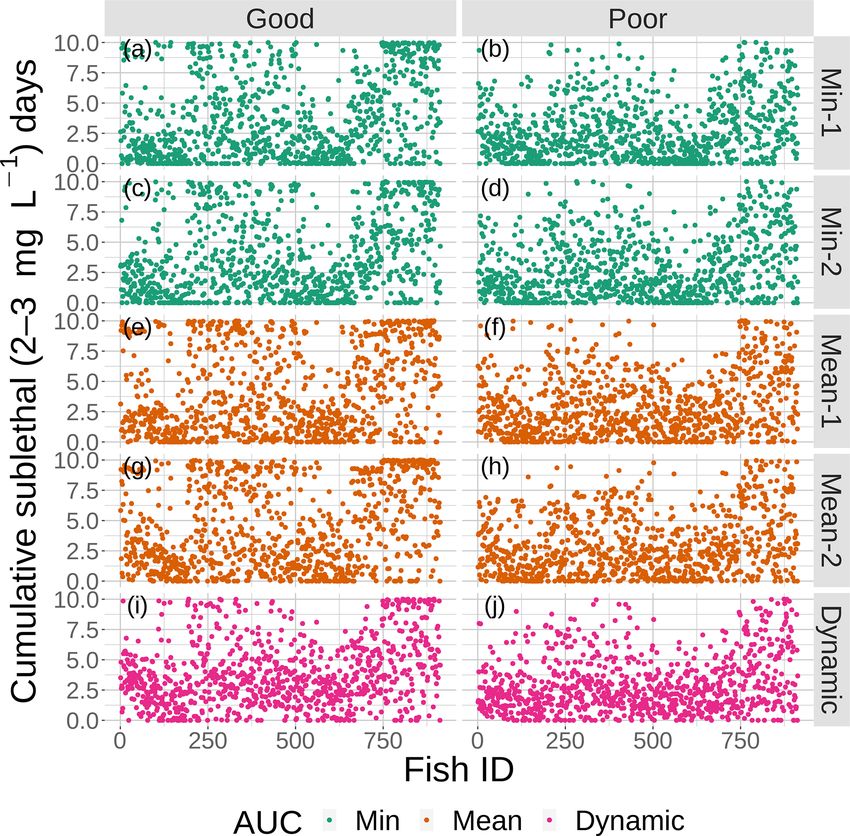
488                                                                           E. D. LaBone et al.: Effects of spatial variability

ification (Rabalais et al., 2001, 2002). Organic matter re-         we find that low DO varies on increasingly finer temporal and
sulting from nutrient-enhanced surface primary production           spatial scales. Understanding these finer scales is relevant for
sinks to the bottom layer where it is respired. Because of          quantifying the exposure of mobile organisms such as fish.
the strong stratification during summertime, oxygen supply             Individual fish are affected both directly and indirectly
is generally lower than respiration, thus creating conditions       by hypoxia. Direct effects of hypoxia on fish include mor-
favorable for hypoxia development (Justic et al., 1996; Ra-         tality, and the sublethal effects of reduced fecundity and
balais et al., 2002). Hypoxia is broken up in the fall by in-       growth (Shimps et al., 2005; Stierhoff et al., 2006; Rose
creased winds associated with cold fronts and cooling of sur-       et al., 2009; Thomas and Rahman, 2012; Limburg and Casini,
face waters. Annual summertime (late July) surveys since            2018, 2019). Fish and other organisms change their move-
1985 have documented a highly variable hypoxic area whose           ment behavior to avoid lethal levels of DO (Eby and Crow-
extent during 1985 to 2011 varied from 700 to 23 200 km2            der, 2002; Bell and Eggleston, 2005; Pollock et al., 2007;
(Table S2 in Obenour et al., 2013). The areal extent of hy-         Craig, 2012). However, while many species avoid hypoxia
poxia is expected to increase under future climate change           (< 2 mg L−1 ), they are still exposed to low DO concentra-
scenarios (Justic et al., 2003, 2016; Sperna Weiland et al.,        tions (2 to 4.5 mg L−1 ) that cause sublethal effects (Vaquer-
2012; Lehrter et al., 2017; Rabalais and Turner, 2019). The         Sunyer and Duarte, 2009; Hrycik et al., 2017). Indirect ef-
interannual variation in hypoxic area in the GOM has been           fects of hypoxia on fish include changes in mortality, growth,
extensively analyzed using regression and simplified semi-          and fecundity that result from avoidance of low DO, caus-
empirical (e.g., box model) methods (Obenour et al., 2015;          ing fish to experience less suitable habitat in their new loca-
Scavia et al., 2017; Del Giudice et al., 2019), as well as with     tions, as well as by direct effects of low DO on their prey and
more complex three-dimensional coupled hydrodynamic–                predators. Hypoxia avoidance can result in fish being forced
biogeochemical models (e.g., Fennel et al., 2013; Justić and       out of preferred habitat to one where there are fewer suit-
Wang, 2014).                                                        able prey and less shelter from predators (Eby and Crow-
   In addition to interannual variation, the hypoxic zone           der, 2002). Hypoxia can also affect the size, growth, energy
within the GOM varies spatially during the summer depend-           demands, and behavior of predators (Pollock et al., 2007;
ing on the interaction of various physical and biological fac-      Breitburg et al., 2009) and the productivity, distribution, and
tors, local bathymetry, wind forcing, hydrodynamics, solar          composition of their zooplankton and benthic prey (Baustian
radiation, river freshwater and nutrient inputs, phytoplankton      et al., 2009; Levin et al., 2009; Roman et al., 2019). While
productivity, and zooplankton grazing (Bianchi et al., 2010).       effects on individuals have been well documented in the lab-
The hypoxic zone typically includes a core area that is hy-         oratory under known and fixed exposures, major challenges
poxic over most summers with outer regions where DO con-            remain to estimate exposure of fish to dynamically changing
centrations are typically more variable in time and space (Ra-      DO in two and three dimensions (Rose et al., 2009; LaBone
balais et al., 2007; DiMarco et al., 2010). Continuous DO           et al., 2019), and to translate these time-varying exposures to
measurements at fixed locations often show rapid changes            growth, mortality, and reproduction effects (Neilan and Rose,
(on the order of ± 1–3 mg L−1 h−1 ) in bottom DO concentra-         2014).
tions (Babin and Rabalais, 2009; Bianchi et al., 2010; Rabal-          The fine-scale temporal and spatial dynamics of DO have
ais et al., 2010; Babin, 2012). Such temporal variations have       been simulated in the GOM using high-resolution, three-
also been documented for other coastal systems (e.g., San-          dimensional (3-D) coupled hydrodynamic–biogeochemical
ford et al., 1990; Booth et al., 2014; Kraus et al., 2015). These   models (Fennel et al., 2016; Rose et al., 2017). These include
temporal variations are caused by the combined effects of lo-       the FVCOM-WASP (Finite Volume Coastal Ocean Model -
cal DO dynamics and the transport of DO via the movement            Water Quality Analysis Simulation Program) model (Justić
of water and therefore imply some degree of spatial variation.      and Wang, 2014) and an implementation of the ROMS (Re-
Spatial analysis of DO measured synoptically at multiple lo-        gional Ocean Modeling System) model coupled with a wa-
cations in the GOM shows various degrees of patchiness in           ter quality and NPZ model (Fennel et al., 2013). FVCOM
hypoxia on kilometer scales (Zhang et al., 2009), and such          is an open-source, unstructured grid ocean circulation model
spatial variation is common in other estuarine systems (e.g.,       (Chen et al., 2011). WASP is a water quality model with a
Muller et al., 2016). Hypoxia in the GOM also varies in the         number of modules, including one for eutrophication (Wool
vertical dimension. For example, the thickness of the hypoxic       et al., 2006). We have previously used the FVCOM-WASP
zone varied from less than a meter to 20 m over the historical      model and added the capability to simulate the fine-scale
record (Fig. S2 in Obenour et al., 2013). Rose et al. (2018b)       movement of individual fish (Justić and Wang, 2014; Rose
summarized continuous measurements of DO obtained using             et al., 2014). The same model setup used here was previously
a towed vehicle (Scanfish) that undulated between 2 m below         used to compare the effects of different movement algorithms
the surface and 2 m above the bottom (Roman et al., 2012;           (LaBone et al., 2017) and 2-D versus 3-D avoidance move-
Zhang et al., 2014), and documented that bottom DO can              ment on fish exposure to hypoxia (LaBone et al., 2019).
frequently change by about 0.5 mg L−1 min−1 on the scale               In this paper, we build upon the analysis of LaBone et al.
of tens of meters. It seems that the more we look, the more         (2017, 2019) and quantify fish exposure to hypoxia and sub-

Biogeosciences, 18, 487–507, 2021                                                       https://doi.org/10.5194/bg-18-487-2021
E. D. LaBone et al.: Effects of spatial variability 489
Figure 1. Planar view of the FVCOM-WASP model grid. There
were also 30 vertical sigma layers.
lethal DO concentrations under different levels of spatial
variability in DO on static maps. For comparison, we also
include the dynamic DO map from which we extracted the
static maps as snapshots. Spatial variability in DO on the
static maps was summarized statistically to ensure that con-
trasting levels of spatial variability were selected for the
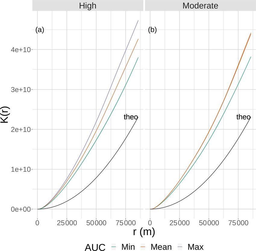
analysis. FVCOM-WASP was used to generate the dynamic Figure 2. The results of Ripley’s K function versus the neighbor-
DO fields within which the individual fish moved and ex- hood size (r) for eight static 2-D snapshot maps of DO from the bot-
perienced static or dynamic (hourly changing) DO concen- tom layer of the FVCOM-WASP simulation of 20–30 August 2002.
trations. Movement of individual fish was modeled every The snapshots are defined in Table 1. Ripley’s K values (lines) are
15 min for 10 d on the static and dynamic maps of DO within shown for maps split into high (a) and moderate (b) sublethal ar-
the same grid as used by FVCOM-WASP. Effects of spatial eas and by AUC values with each panel. There are lines for the two
minimum and single mean and maximum AUC values for the high
variability in DO concentrations on exposure were compared
sublethal area and for the minimum and to mean AUC areas for
for fish with poor versus good avoidance capabilities and
the moderate sublethal area. Some of the curves overlap and are not
with and without an option for vertical avoidance. The re- easily distinguished. The line labeled “theo” represents the relation-
sults for the 2-D (bottom layer) and 3-D (vertical avoidance ship between Ripley’s K and r for the theoretical condition when
allowed) analyses were similar, so here we focus on the 2-D the spatial variability in sublethal DO cells is homogeneous.
results; the 3-D results are summarized in the Supplement.
Our overarching hypothesis was that more spatially variable
DO conditions should result in higher hypoxia and sublethal used from shallow to deep waters; individual fish locations
exposures. However, our results showed that the relationship are also available by depth that is computed from the sigma
between spatial variability and exposure is complex; the ef- layers. The unstructured model grid allows higher resolution
fects of spatial variability on sublethal exposures are highly along the coast and an accurate representation of the GOM
dependent on the areal extent of sublethal DO levels. coastline. The FVCOM-WASP model has been previously
calibrated to accurately represent the circulation and strat-
ification on the shelf (Wang and Justic, 2009). Hourly DO
2 Methods from a 10 d simulation (20–30 August 2002) was used as the
source for the 2-D and 3-D static and dynamic DO maps. The
2.1 FVCOM-WASP 20–30 August 2002 time period had a large hypoxic zone
(∼ 16 000 km2 ) that showed variation at fixed locations on
Output from the coupled FVCOM-WASP model (Justić and hourly and daily timescales. The bottom sigma layer from
Wang, 2014) was used with the FVCOM particle tracking the 3-D FVCOM-WASP model output was used to create 2-
module that was modified to simulate behavioral movement D DO maps for simulating fish movement so that the DO
of individual fish. Individual fish were followed within the values in the bottom layer were identical for the 2-D and 3-D
same 3-D grid that was used for hydrodynamics and the wa- maps.
ter quality modeling. The model domain covered the coastal
GOM from Mobile Bay, Alabama, to Galveston Bay, Texas, 2.2 Movement algorithms
and extended offshore to a depth up to 300 m with the wa-
ter column divided into 30 sigma layers (Fig. 1, Wang and Fish movement was simulated within the FVCOM-WASP
Justic, 2009). Sigma layers vary in their thickness across grid by using a suite of algorithms that determined the veloc-
the model domain because the same number of layers are ities of individual fish in the horizontal plane (u and v) for
https://doi.org/10.5194/bg-18-487-2021 Biogeosciences, 18, 487–507, 2021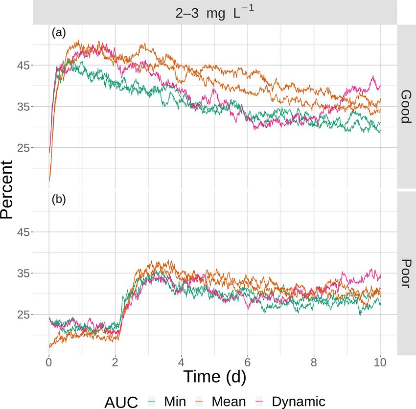
490                                                                               E. D. LaBone et al.: Effects of spatial variability

Table 1. Areas (hypoxic, sublethal, and normoxic; km2 and percent of grid) and AUC (area under the curve) values for eight snapshots
selected from the hourly DO maps generated by FVCOM-WASP simulation of 10 d (20–30 August 2002). Sublethal DO was defined as
2–4 mg L−1 . Based on the sublethal area and AUC values, each snapshot was labeled by category of total sublethal area (S. area; high or
moderate) and by category of AUC (minimum, mean, or maximum).

      Label         Category                                         Area                                              AUC
                                                   km2                                   Percent
               AUC        S. area    Sublethal   Hypoxic    Normoxic       Sublethal    Hypoxic     Normoxic   Sublethal   Hypoxic
      Min-1    Min        Moderate     29 099     15 548       84 619             23          12          66        1.05       1.69
      Min-2    Min        Moderate     29 465     15 460       84 340             23          12          65        1.05       1.69
      Mean-1   Mean       Moderate     31 527     17 166       80 559             24          13          62        1.20       1.70
      Mean-2   Mean       Moderate     31 951     17 341       79 956             25          13          62        1.20       1.68
      Min-1    Mean       High         38 813     19 752       70 630             30          15          55        1.04       1.52
      Min-2    Mean       High         38 667     19 869       70 659             30          15          55        1.04       1.51
      Mean     Mean       High         38 083     16 972       74 156             30          13          57        1.19       1.80
      Max      Mean       High         36 748     16 300       76 168             28          13          59        1.34       1.90

2-D and additionally using the vertical velocity (w) for the            computed (e1 and e2), and these were used to select among
3-D simulations (Rose et al., 2014; LaBone et al., 2019). The           three avoidance algorithms (NS, Sprint, and CRW) depend-
changes in fish position were calculated by updating their              ing on the severity of hypoxia exposure. When none of the
previous time step’s positions on the grid with the newly               three DO-related algorithms for avoidance were selected, the
computed velocities to obtain the new positions of the fish             individual used the default movement algorithm (CCRW)
(Watkins and Rose, 2013; Rose et al., 2014). In 2-D, the                that was unrelated to DO conditions. The cuing variables e1
equations are                                                           and e2 were binary variables (zero or one) computed on each
                                                                        time step (every 15 min) for each individual, with e1 being
x(t + 1t) = x(t) + u(t) · 1t,                                 (1)       triggered when the DO concentration in the cell (exposure
y(t + 1t) = y(t) + v(t) · 1t,                                 (2)       now) was less than 2 mg L−1 , and e2 was triggered when
                                                                        an individual’s cumulative exposure to DO < 2 mg L−1 ex-
where x and y were the fish positions on the model grid (dis-           ceeded a continuous 48 h. Thus, each individual had its own
tance in meters from bottom left-hand corner of grid), u and            evolving time series of zero or one values for each cue (e1
v are the velocities in the x and y directions, and 1t is the           and e2).
time step (15 min). The velocities u and v were calculated
each time step as                                                       2.2.2   Neighborhood search

u(t) = ss · cos(θ (t)),                                       (3)       When the NS algorithm was selected by the event-based al-
v(t) = ss · sin(θ (t)),                                       (4)       gorithm it was considered a tactical (immediate and urgent)
                                                                        response because the individual fish was about to be ex-
where ss was the swimming speed (m s−1 ) and θ was the                  posed to DO < 2 mg L−1 . The individual then searched the
swimming angle (radians) relative to the x axis. The swim-              surrounding cells for the one with the lowest DO value and
ming speed and swimming angle were computed differently                 moved in the opposite direction at a swim speed twice the
among the algorithms, and which algorithm to use was se-                baseline (default) speed. The angle and swimming speed
lected based on the DO concentrations experienced by the                were calculated as
fish. The collection of algorithms to model fish movement
                                                                        θ (t) = atan2(y(t) − yl(t), x(t) − xl(t))
and exposure to DO were the same as used in previous anal-
yses (LaBone et al., 2017, 2019).                                       + 0.15 · 2π(2 · ran − 1),                                     (5)
                                                                        ss = 2 · ss0 ± ss0 · ran,                                     (6)
2.2.1    Event-based movement
                                                                        where x(t) and y(t) are the current x and y coordinates, xl(t)
An event-based algorithm was used to choose among the var-              and yl(t) are the coordinates of the center of the cell with the
ious algorithms that computed swim speed and angle. There               lowest DO, ss0 is the default swim speed, and ran is a uniform
were four possible algorithms that an individual fish could             random number. The first part of Eq. (5) (atan2), calculates
use on a time step: neighborhood search (NS), Sprint, cor-              the angle and the second part of the equation calculates a
related random walk (CRW), and Cauchy CRW (CCRW).                       random component that adds some variability to the angle.
On each time step, two cues for DO-related movement were                The NS algorithm is efficient at avoiding hypoxia, but fish

Biogeosciences, 18, 487–507, 2021                                                            https://doi.org/10.5194/bg-18-487-2021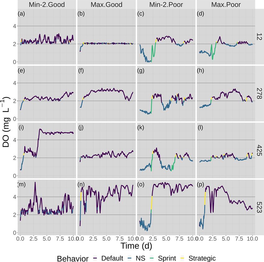
E. D. LaBone et al.: Effects of spatial variability                                                                             491

could get stuck in local maxima that were still hypoxic. The        turning angle from a non-uniform, wrapped Cauchy distribu-
random component added to the swimming angle prevented              tion. The turning angle and swimming speed were calculated
most, but not all, fish from getting stuck at local hypoxic cells   by
that were also the local maximum DO concentration.
                                                                    θ (t) = θ (t − 1t) + 2 · atan
2.2.3    Sprint
                                                                       (1 − )
                                                                               · tan((ran − 0.5) · π ) + θm ,                  (11)
The Sprint algorithm was also considered a tactical response           (1 + )
to hypoxia exposure and was selected when an individual fish
spent too long in the hypoxic waters, often the result of being
stuck at local hypoxic maxima from which the NS algorithm
could not successfully move fish to non-hypoxic waters. If          ss = ss0 ± 0.3 · ss0 · ran,                                (12)
the fish spent more than 48 continuous hours in hypoxic con-
ditions, the fish would swim quickly (3 times the default           where  determines the shape of the wrapped Cauchy distri-
speed) in a straight line out of the hypoxic zone going in          bution and θm determines the center of the distribution. θ (t-
the direction the fish last traveled. The angle and swimming        1t) is the previous angle and the 2 · atan[] + θm is the turning
speed were calculated as                                            angle. Higher values of  result in more correlation and less
                                                                    randomness to the direction of the fish. The value assigned
θ(t) = θ (t − 1t),                                           (7)    to θm determined the bias in whether the individual tended to
ss = 3 · ss0 .                                               (8)    turn left or right.

The fish used Sprint on successive time steps until it exited       2.2.6    Reflective boundary
the hypoxic zone, when its continuous exposure to hypoxia
was reset back to zero.                                             Reflective boundary was an application of the NS algorithm
                                                                    used to reflect fish back into the model domain. Reflective
2.2.4    CRW                                                        boundary was used outside of the event-based algorithm and
                                                                    was applied after all of the other algorithms for fish move-
CRW was a biased random walk algorithm (Kareiva and                 ment were applied and the individual was placed in its new
Shigesada, 1983) used for a strategic response to hypoxia.          location. The reflective boundary algorithm would be trig-
A strategic response is considered a response to hypoxia ex-        gered when a fish was determined to have moved outside of
posure but when the exposure is not immediate (like with            the model domain. The fish was moved back to its position
tactical) but rather had occurred in the recent past. CRW, as       at the start of the time step, and then the surrounding cells
a strategic response, typically followed the tactical NS re-        were searched and the fish moved to the cell with the fewest
sponse because once the immediate threat of exposure was            boundaries. The angle was calculated as
gone, there was still some memory of the immediate expo-
sure and the individual was likely in an area where there           θ (t) = atan2(yl(t) − y(t), xl(t) − x(t))
was hypoxia. The CRW algorithm had fish continue to swim
away (at the relatively slower default speed) from hypoxic          + 0.15 · 2π · (2 · ran − 1),                               (13)
areas after NS enabled the fish to exit hypoxic conditions.
CRW used the velocities from the previous time step to cal-         where the values are the same as Eq. (5). The only change
culate the angle and calculated a random speed:                     in the calculation of θ as compared to NS was the order of
                                                                    coordinate values in the atan2 function. Speed was calculated
θ(t) = atan2(v(t − 1t), u(t − 1t))                                  using the default swim speed (ss0 ).
+ 0.05 · 2π · (2 · ran − 1),                                 (9)
                                                                    2.3     Algorithm selection
ss = ss0 ± 0.3 · sss0 · ran.                                (10)

The first half of Eq. (9) (atan2( )), are the velocities from the   The event-based algorithm chooses the movement algorithm
previous time step and the second part of the equation is a         that has the highest utility for each time step. Utilities are
random component to add variation to the angle.                     used to represent the costs and benefits that a particular be-
                                                                    havior has on an animal’s fitness (Anderson, 2002). For our
2.2.5    Default                                                    purposes of avoidance of low DO, we only considered that
                                                                    avoiding hypoxia was critical to fitness. In evaluating the dif-
CCRW was the random walk algorithm used as a default                ferent algorithms, we did not factor in the costs of avoiding
movement in the model and is a more complicated biased              hypoxia or how decisions would affect growth, mortality, or
random walk than CRW (Wu et al., 2000). The magnitude               reproduction. We computed three utility values for each time
and direction of the bias can be controlled by choosing the         step based on the probabilities of two events indicative of

https://doi.org/10.5194/bg-18-487-2021                                                            Biogeosciences, 18, 487–507, 2021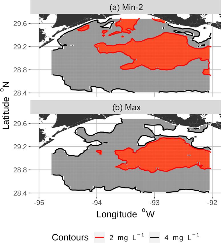
492                                                                           E. D. LaBone et al.: Effects of spatial variability

immediate (e1) and prolonged (e2) exposure occurring:

UNS (t) = utilNS · probNS (t),                              (14)
Usprint (t) = utilsprint · probsprint (t),                  (15)
UCRW (t) = utilCRW · probCRW (t),                           (16)

where utili is the intrinsic utility and probi is the probability
of a triggered event. The intrinsic utility is the weight each
algorithm has in the utility calculation. Tactical algorithms
have a higher weight than default or strategic algorithms and
thus are preferentially chosen. The probability of an event
being triggered was calculated for NS and CCRW using the
event of immediate exposure (e1):

probNS (t) = (1.0 − memNS ) · e1(t)
+ memNS · probNS (t − 1t),                                  (17)
probCRW (t) = (1.0 − memCRW ) · e1(t)
+ memCRW · probCRW (t − 1t).                                (18)

   The probability for Sprint used event two (e2):

probsprint (t) = (1.0 − memsprint ) · e2(t)
+ memsprint · probsprint (t − 1t).                          (19)    Figure 3. Spatial maps of bottom DO showing the 2 and 4 mg L−1
                                                                    contours for two of the eight snapshots from the FVCOM-WASP
The three probabilities are running averages of present and         simulation of 20–30 August 2002. The snapshots are defined in Ta-
recent past hypoxia exposures and allow for the fish to have        ble 1. Snapshot Min-2 (a; row 2 in the Table) is moderate sublethal
some memory of past events. The utilities on each time step         area and minimum AUC, and snapshot Max (b; row 8 in the Table)
                                                                    is high sublethal area and maximum AUC. Areas in white outside
were then compared and the algorithm with the largest util-
                                                                    the 4 mg L−1 line are normoxic.
ity value that exceeded a minimum threshold was selected. If
none of the calculated utilities were larger than the threshold
(hypoxia exposure was not imminent and had not occurred in
the recent past), then the default behavior was used. Parame-       case, we have a 2-D spatial map of cells that are either hy-
ters for Eqs. (14) to (19) are given in Table 2.                    poxic, sublethal, or normoxic. We computed the Ripley’s K
                                                                    based on whether cells were sublethal or not. Ripley’s K
2.4   Selection of static DO snapshots                              measures the number of extra sublethal cells (above that ex-
                                                                    pected under randomly distributed sublethal cells) within a
Eight static DO snapshots were selected from the 240 hourly         fixed distance (r, in meters) of a randomly chosen cell. Thus,
snapshots simulated during the 10 d (20–30 August 2002)             Ripley’s K used here is a method for quantifying the spa-
FVCOM-WASP simulation (Table 1). For each snapshot, a               tial distribution of sublethal cells on a map compared to the
2-D map and a 3-D map of DO were created. The snap-                 sublethal cells showing complete spatial randomness (CSR).
shots were selected based on a combination of the total             As an aid in interpretation, our computed Ripley’s K was
area of sublethal DO and the degree of spatial variability          compared to the theoretical value expected if the sublethal
in DO on each of the 240 2-D maps. Area based on the                cells were spatially homogenous (Ktheo ; Fig. 2). If our com-
full range of sublethal concentrations (DO of 2–4 mg L−1 ),         puted K is less than Ktheo , then the sublethal cells are spa-
and also the hypoxic area (DO < 2 mg L−1 ) and normoxic             tially dispersed and sublethal cells are, on average, farther
area (DO > 4 mg L−1 ) for reference and comparison, were            apart than expected compared to a random distribution. If
computed for each hourly time step. Also for each of the            our computed K for a map is greater than Ktheo , then there is
240 time steps (spatial maps of DO), Ripley’s K func-               clustering of sublethal cells and sublethal cells generally oc-
tion (Kest in R; https://www.rdocumentation.org/packages/           cur closer together (clumped) than expected under random-
spatstat/versions/1.63-3/topics/Kest, last access: 29 Novem-        ness (Brunsdon and Comber, 2015). To obtain a single value
ber 2020), with isotropic edge correction, was computed,            for a map as an indicator of spatial variability so we could
which resulted in the plots of the statistic K versus r. Rip-       easily compare spatial variability across the 240 maps, we
ley’s K is an estimation of the K function that accounts for        used the area under the curve (AUC) relating Ripley’s K to
maps with finite area and includes edge corrections. In our         r for each map. By using AUC that summarizes over a wide

Biogeosciences, 18, 487–507, 2021                                                        https://doi.org/10.5194/bg-18-487-2021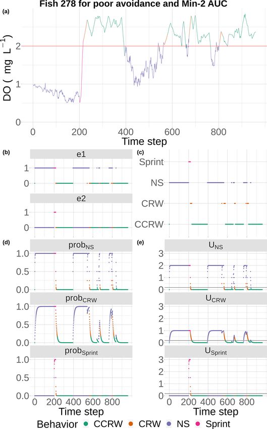
E. D. LaBone et al.: Effects of spatial variability                                                                                 493

Table 2. Parameter values for the four movement algorithms used to simulate avoidance of low DO and the default behavior of individual
fish.

                Parameter           Value     Description                                                      Equation(s)
                ss0                   0.23    Baseline (default) swimming speed (m s−1 )                          6, 8, 10
                                       0.9   Determines if wrapped Cauchy distribution is circular or ovoid            11
                θm                        0   Determines direction of bias of wrapped Cauchy distribution               11
                util                2, 3, 1   Utility weight for NS, Sprint, and CCRW algorithms                14, 15, 16
                mem           0.5, 0.5, 0.9   Memory weight for NS, Sprint, and CCRW algorithms                 17, 18, 19

                                                                        maximum AUC values (Fig. 2). The duplicate snapshots for
                                                                        a given AUC provide information on the variability of simu-
                                                                        lation results when two different maps have similar sublethal
                                                                        areas and AUC values. Figure 3 illustrates the spatial vari-
                                                                        ability in DO using maps of sublethal DO for one of the
                                                                        minimum AUC (Min-2) snapshots for the moderate sublethal
                                                                        area and another for the maximum AUC (Max) with the high
                                                                        sublethal area. The larger area of sublethal concentrations is
                                                                        seen by the larger area of gray in Fig. 3b versus Fig. 3a. When
                                                                        we visually compared maps of low versus high AUC for the
                                                                        same sublethal area (high or moderate), differences in the
                                                                        degree of clustering of sublethal areas between low and high
                                                                        AUC values were not obvious. Figure 4 shows a blown-up
                                                                        area that illustrates the higher clumpiness and patchiness in
                                                                        sublethal DO when the AUC value is higher. The gray area
                                                                        in Fig. 4b (AUC of 1.67 × 10⁹) shows more irregular bound-
                                                                        aries, especially in the top left and right portions of the sub-
                                                                        lethal area, versus Fig. 4a (AUC of 1.33 × 10⁹).

                                                                        2.5    Design of simulations

                                                                        Movement, and the associated exposure to DO, was simu-
                                                                        lated using 913 individual fish for 10 d on each of the eight
Figure 4. Zoomed-in view of spatial maps of bottom DO showing           static maps and the dynamic version. The number of fish was
the 2 and 4 mg L−1 contours for two of the eight snapshots from the
                                                                        determined by placing a regular grid of fish locations onto
FVCOM-WASP simulation of 20–30 August 2002. The snapshots
                                                                        the model domain and removing any that were assigned to
are defined in Table 1. Snapshot Min-2 (a; row 2 in the Table) is
moderate sublethal area and minimum AUC, and snapshot Max (b;           land cells. The starting positions of the individuals were de-
row 8 in the Table) is high sublethal area and maximum AUC. Areas       termined by using an algorithm that had fish move towards a
in white outside the 4 mg L−1 line are normoxic.                        preferred temperature (LaBone et al., 2017). Fish movement
                                                                        was simulated for several days until the temperature-seeking
                                                                        movement algorithm reached steady state with fish gathered
                                                                        along the 26 ◦ C contour line that was specified as their op-
range of neighborhood sizes, larger AUC values imply the                timal temperature. This enabled initial starting locations to
map has greater spatial variability (more clumpiness) in its            be spread out over the domain while preserving a relatively
distribution of sublethal DO concentrations.                            realistic initial spatial distribution expected without hypoxia.
   To select the eight snapshots, we plotted AUC versus                 Simulations were done for the 2-D and 3-D maps and for
sublethal area and identified eight snapshots with moderate             good and poor avoidance competency. Good avoidance used
and high sublethal areas that corresponded to the minimum,              the NS as described, while poor avoidance competency was
mean, and maximum AUC values (Table 1). For moderate                    achieved by changing the 0.15 value in Eq. (5) to 0.5, result-
sublethal areas we selected two snapshots with minimum                  ing in a much wider randomly generated direction of move-
AUC and two snapshots with mean AUC; the maximum                        ment during avoidance. Fish positions were updated every
AUC was similar to the mean so no maximum was selected.                 15 min, and DO in the dynamic maps changed every hour. We
For the high sublethal area case, two snapshots were matched            present the results for the 2-D set of maps; similar patterns
with minimum AUC and single snapshots with mean and                     of spatial variability of effects on exposure were obtained

https://doi.org/10.5194/bg-18-487-2021                                                              Biogeosciences, 18, 487–507, 2021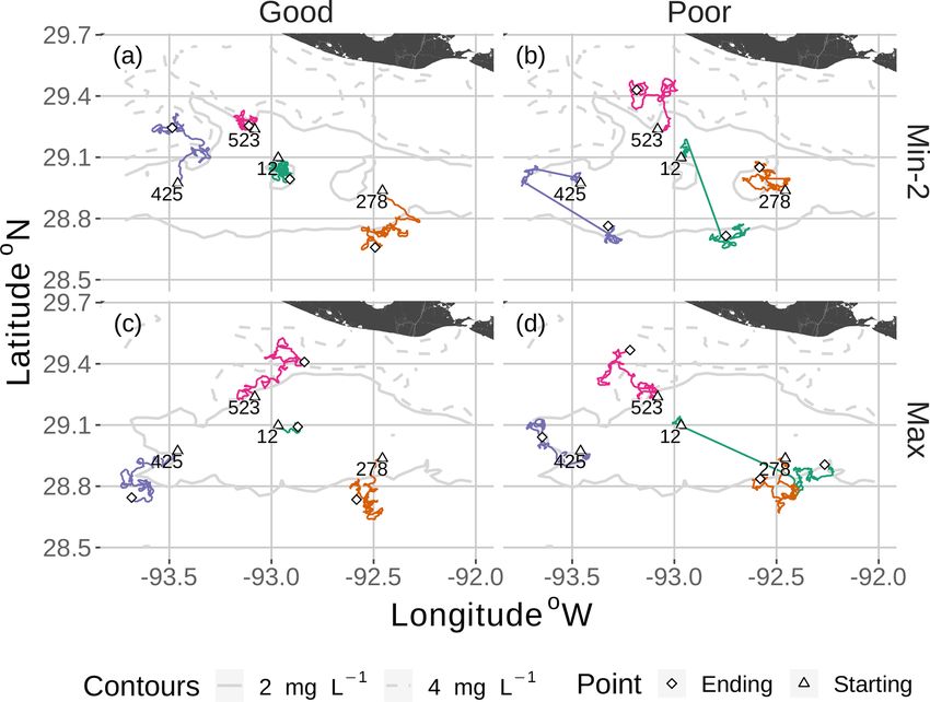
494 E. D. LaBone et al.: Effects of spatial variability
for the 3-D set of maps (Supplement). Movement parame-
ters were set to values typical for croaker and related species
(Table 2). Croaker is an abundant demersal-oriented fish in
coastal waters of the northern GOM, especially in coastal
waters off of Louisiana where hypoxia occurs annually. Ex-
tensive laboratory and field data available for DO effects on
croaker have been previously used to specify realistic val-
ues for movement-related parameters (Rose et al., 2018b, a;
LaBone et al., 2017, 2019).
Model outputs of fish locations and DO experienced every
15 min were analyzed to determine how spatial variability in
DO affected exposure to hypoxia and sublethal DO concen-
trations. To illustrate the movement behavior, we show the
detailed movement calculations (e1, e2, and the three prob-
abilities and utilities) for a single fish for poor competency
on a single static map (Min-2 of moderate sublethal area)
and the movement tracks and DO experienced for four indi-
vidual fish for good and poor avoidance on two of the static
DO snapshots. The DO experienced was color coded to show
which movement algorithm was being used over time.
Exposure of all individuals was summarized over the 10 d
for each fish by their cumulative exposure, which was cal-
culated as the sum of the number of 15 min time steps (ex-
pressed as days) each fish was exposed to DO less than
2 mg L−1 . Cumulative exposure to sublethal conditions was
calculated the same as the exposure to hypoxia, except the
overall sublethal range of 2–4 mg L−1 (sublethal) was sub-
divided into 2–3 mg L−1 and 3–4 mg L−1 , and each of these
was considered the “exposed”. We show plots of the cumu-
lative exposure of all individual fish and also boxplots that
summarize cumulative exposures over all fish. Outlier values
were displayed in the box plots as points beyond the whiskers
of the plot and were identified as values outside 1.5 · IQR (in-
Figure 5. DO experienced and the component calculations used by
terquartile range). The outliers are considered extreme but
the event-based algorithm to select movement algorithms at every
usable values, as they were not questionable or suspicious
15 min time step for fish 278 under the conditions of poor compe-
“outlier” values in the statistical sense, and were therefore tency and minimum AUC (Min-2) maps with moderate sublethal
included in all analysis of model outputs. Another summary area. DO is used each time step (a) to determine e1 and e2 (b), with
of the exposure output was the percentage of fish on each e1 used to compute the probabilities for NS (tactical) and CRW
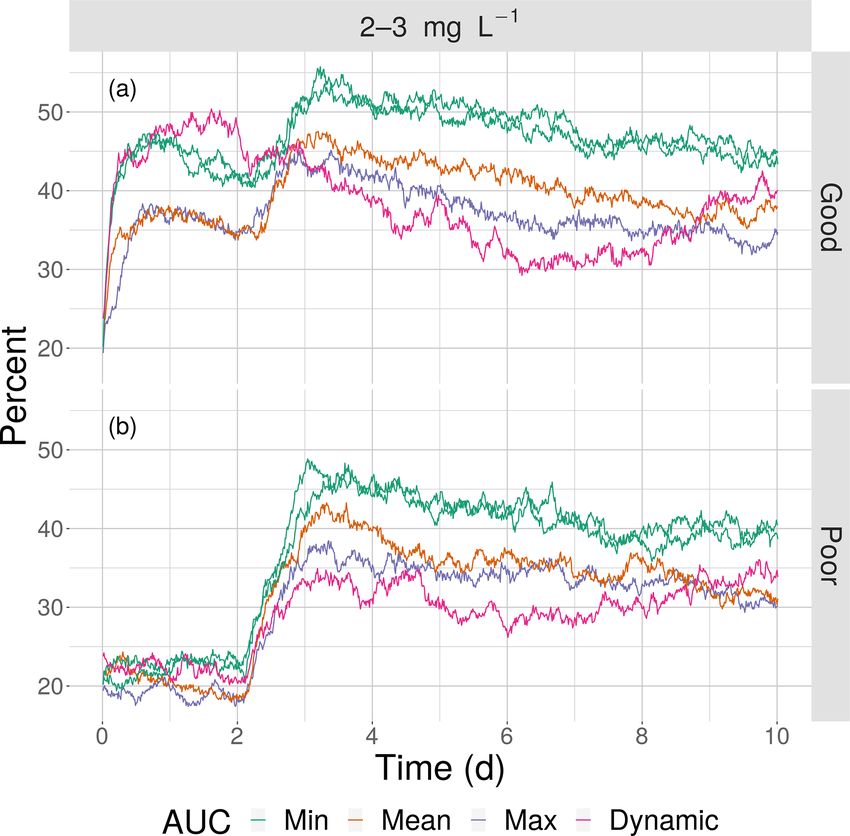
time step between 2–3 mg L−1 . We focus on the 2–3 mg L−1 (strategic) avoidance and e2 used to compute the probability for
range for the sublethal analysis in this paper because it would Sprint (d). These probabilities are used to compute utilities for the
have the most ecological effects on individuals (just above three algorithms each time step, (e) and the algorithm with highest
lethality) and the results for 3–4 mg L−1 were consistent with utility above a minimum threshold is selected to be used for move-
2–3 mg L−1 but showed less overall variation and so the pat- ment for that time step (c). If none of the three avoidance-related
terns were less clear. R was used for all statistical analysis algorithms are selected, then a fourth algorithm (CCRW) that is un-
related to DO concentration is used.
and graphs (R Core Team, 2019).
3 Results also showed a slower rising utility for the CRW (strategic)
as the fish’s past exposure was considered. When the fish
3.1 Hypoxia avoidance in 2-D was unable to avoid waters with DO < 2 mg L−1 for 2 d (time
step = 192, Fig. 5a), Sprint got invoked (Fig. 5b, c). Once
Fish movement was a mix of the different behaviors, depend- the fish entered waters with DO > 2 mg L−1 using Sprint, the
ing on the DO conditions they encountered (Figs. 5 and 6). utilities for both NS and CRW avoidance movement quickly
Our example fish (Fig. 5) was immediately exposed to hy- returned to zero as exposures to DO > 2 mg L−1 accumulated
poxia that triggered the NS tactical avoidance (via e1) and (Fig. 5e). The fish then used default (CCRW) while moving
Biogeosciences, 18, 487–507, 2021 https://doi.org/10.5194/bg-18-487-2021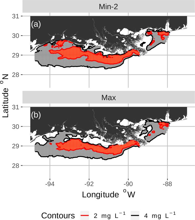
E. D. LaBone et al.: Effects of spatial variability                                                                                   495

Figure 6. Time series of DO experienced by the four fish shown in Fig. 7 over the 10 d of the model for good and poor avoidance and the two
snapshot DO maps (Min-2 for moderate sublethal and Max for high sublethal area). The color of the lines denotes the movement algorithm
that each individuals was using. Black lines denote the thresholds for hypoxia (2 mg L−1 ) and the upper value (4 mg L−1 ) considered for
sublethal concentrations.

among cells with DO > 2 mg L−1 (Fig. 5c). At time step 400,             randomness) had to use Sprint (perfectly straight path) af-
the fish wandered into water with DO < 2 mg L−1 , causing               ter spending 48 h in hypoxic conditions. Several of the se-
the utilities for NS and CRW to rise (Fig. 5e) and trigger-             lected fish used a mix of all four algorithms (all fish in Min-
ing NS for an extended time period (time steps 475 to 600,              2 with poor competency), while other individuals used two
Fig. 5c) as the fish moved around trying unsuccessfully to              or fewer algorithms that were dominated by default move-
avoid waters with DO < 2 mg L−1 . Once NS enabled the fish              ment. The exposure patterns and variability in DO experi-
to move to waters with DO > 2 mg L−1 , CRW would briefly                enced also varied among individuals, even though these were
get triggered because of its history of exposure (Fig. 5c). Sev-        maps with fixed spatial distributions of low DO. For exam-
eral more times the pattern of NS and CRW (both avoidance)              ple, individual no. 12 (Fig. 6b), after escaping hypoxia ex-
were triggered (Fig. 5c, e), mostly keeping the fish in wa-             posure, was exposed to DO just above 2 mg L−1 throughout,
ters with DO > 2 mg L−1 , except for a few brief time periods           while other individuals on certain maps (e.g., 425 on Min-
(Fig. 5a). While the fish generally avoided hypoxia after the           2 with good competence, Fig. 6i) eventually went to waters
initial exposure and during the one extended period of hy-              with DO > 4 mg L−1 .
poxia exposure (time steps 475 to 600), the fish was then
always exposed to sublethal levels (2–4 mg L−1 ) throughout             3.2   Hypoxia exposure
the 10 d.
   DO experienced and fish trajectories (Figs. 6 and 7) il-             Cumulative exposure of individuals to hypoxia was higher
lustrated how a fish with good avoidance used NS (mostly                under the high sublethal area snapshots compared to the
straight path with some randomness) to escape the hypoxic               moderate sublethal snapshots, with good competence show-
zone, while several of the fish with poor avoidance (higher             ing the greater difference between moderate and high. With

https://doi.org/10.5194/bg-18-487-2021                                                             Biogeosciences, 18, 487–507, 2021
496                                                                             E. D. LaBone et al.: Effects of spatial variability

                                                                       of opposite effects of spatial variability on hypoxia exposure
                                                                       being dependent on the degree of sublethal area, which is
                                                                       weak here, will become more apparent when sublethal expo-
                                                                       sure is examined.

                                                                       3.3   Sublethal exposure

                                                                       The effects of spatial variability on cumulative sublethal ex-
                                                                       posure to 2–3 mg L−1 of individuals showed higher exposure
                                                                       for high sublethal area (as expected – simply more possibility
                                                                       of exposure) and a tendency for opposite effects of variability
                                                                       between high and moderate sublethal areas. For poor avoid-
                                                                       ance and especially for good avoidance competency, there
                                                                       was a subtle but consistent shifting to lower exposures with
                                                                       increasing variability for high sublethal area (points shifting
                                                                       to lower values from top to bottom in Fig. 10), while there
Figure 7. Movement tracks taken by four fish for good and poor         was a shifting to higher exposures for the moderate sublethal
hypoxia avoidance (left versus right) and two snapshots (Min-2 for     area maps (less open space near top of each plot, except
moderate sublethal area and max AUC for high sublethal area). All      for dynamic, in Fig. 11). The pattern of fish with ID values
four fish start (triangle symbol) in the hypoxic zone. These are the
                                                                       greater than 750 having higher exposures to sublethal DO in
same maps as shown in Fig. 3, but here they only show a portion of
                                                                       Figs. 10 and 11 was due to the how individuals were num-
the model grid.
                                                                       bered in the simulation and how they related to where they
                                                                       were initially placed on the grid. High-numbered individuals
                                                                       were generally located closer to hypoxia and sublethal con-
good avoidance competency, almost all fish showed expo-                centrations at the start of the simulations.
sures of about 1–2 d for maps with high sublethal area                    This opposite effect of variability was more apparent when
(Fig. 8a), which were further reduced to almost no expo-               the exposures of fish to 2–3 mg L−1 was examined as the
sure to hypoxia for moderate sublethal area maps (Fig. 9a).            percent of all individuals. Under high sublethal area, the
Sublethal area was positively correlated with hypoxic area,            percent of fish exposed to 2–3 mg L−1 decreased with in-
while both were somewhat negatively related to normoxic                creasing variability for both good competency (Fig. 12a) and
area (Table 1). Poor avoidance resulted in much more similar           poor competency (Fig. 12b). The green lines (min AUC, low
exposures between high and moderate sublethal conditions               variability) had the highest exposure, while the purple lines
(Figs. 8b and 9b), which reflected that the fish have more             (max) and magenta lines (dynamic map) had the lowest ex-
randomness to their avoidance movement that masks some                 posures. For good competency, the averaged percent of indi-
of the differences between the moderate and high sublethal             viduals exposed to 2–3 mg L−1 over the 10 d was 46 % and
area maps. Because of the effects of Sprint being triggered            47 % for the two min variability maps, 39 % for the mean
after the first 48 h for some fish under poor competency, we           map, and 37 % for the max map. A similar range (maxi-
also examined the results using days 3 through 10 (Supple-             mum minus minimum) of averaged percent exposed of about
ment). The patterns in the results described for hypoxia expo-         8 % occurred with poor competency: 37 % and 38 % for min
sure were less pronounced for the good competency results              variability, 32 % for mean, and 30 % for the max map. In
because there was little exposure to hypoxia after the first           both cases, the percent exposure for the dynamic maps were
48 h when fish moved out of hypoxia and were effective at              within the values of their respective static maps (38 % for the
avoiding further exposure. However, removing the effects of            good competency and 29 % for poor competency).
the initial triggering of Sprint for poor competency simula-              The opposite pattern was predicted for the moderate sub-
tions only slightly lowered overall hypoxic exposure, as fish          lethal area conditions (Fig. 13); percent exposed to 2–
continued to be exposed to hypoxia intermittently but with             3 mg L−1 increased, rather than decreased, with increasing
similar percentage of individuals throughout the 10 d.                 variability. In Fig. 13, the green lines (2 min AUC maps)
   The effects of different degrees of spatial variability on          showed the lowest exposures while the orange line (mean
hypoxia exposure were small. There was a weak suggestion               AUC) and magenta line (dynamic) showed the highest expo-
that exposure to hypoxia decreased with increasing variabil-           sures. For good competency, the averaged percent of individ-
ity with the high sublethal area maps but increased with in-           uals exposed to 2–3 mg L−1 was 36 % for the two min vari-
creasing variability for moderate sublethal area maps. This            ability maps and 40 % and 43 % for the mean maps, a range
is seen by the tendency for exposure to decrease from left to          of about 8 %. For poor competency, there was little differ-
right in each panel of Fig. 8, while exposure tended to in-            ence in percent exposed from min and mean maps: 28 % for
crease from left to right in each panel of Fig. 9. This pattern        the two min maps and 29 % for the two mean maps. This lack

Biogeosciences, 18, 487–507, 2021                                                          https://doi.org/10.5194/bg-18-487-2021
E. D. LaBone et al.: Effects of spatial variability 497
Figure 8. Boxplots of cumulative hypoxia exposure of all individu- Figure 9. Boxplots of cumulative hypoxia exposure of all individu-
als (days) for good and poor competency on the four DO snapshot als (days) for good and poor competency on the four snapshot DO
maps with high sublethal area. The cumulative exposure for the sim- maps with moderate sublethal area. The cumulative exposure for
ulation using the dynamic map is also shown. The lower and upper the simulation using the dynamic map is also shown. The lower and
lines of the boxplots show the 25th and 75th percentile value of cu- upper lines of the boxplots show the 25th and 75th percentile value
mulative exposure and the center line is the median. Individual fish of cumulative exposure, and the center line is the median. Individ-
values flagged as extreme values are shown as individual points. ual fish values flagged as extreme values are shown as individual
The star symbol denotes the mean. points. The star symbol denotes the mean.
of a difference was also due to the inclusion of the first 2 d ous area of hypoxia now reveals itself to have a much more
when exposure was similarly low on all of the maps due to spatial structure. The persistence at a location, the dissipation
Sprint, but the differences after day 2 were still not strong. and reforming of hypoxia in response to weather events, local
The opposite effects of spatial variability between moder- bathymetric influences (e.g., Virtanen et al., 2019), and other
ate and high sublethal areas were maintained for 3-D sim- factors, all contribute to the spatial variability in the hypoxic
ulations, and the effects were maintained, but smaller, for and sublethal DO concentrations (Bianchi et al., 2010; Ra-
exposure to 3–4 mg L−1 . The patterns for exposure to 2– balais and Turner, 2019). The rather smooth looking earlier
3 mg L−1 were maintained after the first 48 h of exposures, so annual spatial maps obtained from monitoring data (e.g., Ra-
that Sprint was not overly influential on the patterns, and also balais et al., 2001) are continually evolving into more irreg-
under 3-D conditions, demonstrating the results were robust ular shapes with highly dynamic boundaries and patchiness
to including an option for vertical avoidance (see the Supple- (Zhang et al., 2009; Obenour et al., 2013; Justić and Wang,
ment). For both moderate and high sublethal areas, the oppo- 2014). Further, while we focus on the hypoxic waters, most
site effects of spatial variability were similar but less appar- mobile organisms show avoidance behavior, making the dy-
ent for exposure to 3–4 mg L−1 because exposures in general namics of sublethal concentrations (often not avoided) highly
showed less variation among simulations for 3–4 mg L−1 (re- relevant ecologically. Hypoxia causes mortality, which is a
sults not shown). major consideration at the population level, but the popula-
tion effects also depend on the fraction of the population that
is exposed. Reduced growth, lowered fecundity, and indirect
4 Discussion effects from displacement may have a less obvious influence
on the population than mortality, but if a much larger percent
The spatial variability of DO in the Gulf of Mexico, and of the population are exposed, these sublethal effects can lead
likely in other places with chronic river-driven seasonal hy- to ecologically significant population-level responses that,
poxia, is patchier than we envisioned. As measurements be- in some cases, can exceed the effects from direct mortal-
come more resolved and hydrodynamic water quality models ity (Rose et al., 2009). Fish movement, spatial variability in
become more detailed, what was once considered a continu- DO, and exposure to hypoxia and sublethal concentrations
https://doi.org/10.5194/bg-18-487-2021 Biogeosciences, 18, 487–507, 2021498 E. D. LaBone et al.: Effects of spatial variability
Our refined view of how spatial variability affects expo-
sure distinguishes between hypoxia and sublethal exposures
and shows that effects of spatial variability on sublethal ex-
posure can reverse depending on the areal extent of low DO
waters. Model simulations showed that exposure to hypoxia
was, as expected, greatly influenced by the swimming avoid-
ance competency assumed for the fish. Given other condi-
tions were the same, good competency (little randomness to
avoidance response) resulted in less exposure to hypoxia than
poor competency (left versus right panels in Figs. 8 and 9).
Further, good competency essentially eliminated exposure to
hypoxic conditions. Almost all exposure to hypoxia occurred
in the first 24 to 48 h, and this was generally low (Fig. 8a).
Beyond the initial exposures (i.e., using days 3–10), good
competency resulted in near-zero exposure to hypoxia (see
the Supplement). In contrast, exposure to hypoxia with poor
competency showed persistent and relatively high exposure
to hypoxia that occurred throughout the 10 d of the simula-
tions (results not shown). Such persistent exposure occurred
even when the effects of initial use of Sprint in the first 48
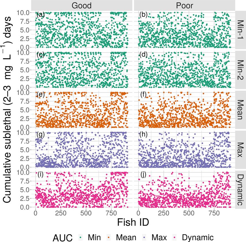
Figure 10. Cumulative exposure (days) of each individual fish to hours were eliminated (see the Supplement).
DO concentrations of 2–3 mg L−1 for good (left) and poor (right) Despite the differences in exposure to hypoxia with good
competency for each of the four snapshot DO maps with high sub- versus poor competency, both resulted in relatively high ex-
lethal area and the dynamic version. Maps within the same AUC posures to sublethal DO concentrations. Roughly, 30 % to
category (the two “Min” maps) are shown with the same color. 50 % of the individuals were exposed to 2–3 mg L−1 and this
occurred, except for the 48 h that triggered Sprint, through-
out the 10 d of almost all of the simulations (Figs. 12 and
are complicated. However, knowing exposure is critical in 13). Interestingly, the percent of individuals exposed to 2–
order to make accurate predictions of the effects of low DO 3 mg L−1 was often somewhat higher (about 5 %–10 %) for
on individuals, which then can be scaled to the responses good competency compared to poor competency. The reason
of populations and food webs (Rose et al., 2009, 2018b, a; is that good competency resulted in fewer individuals being
De Mutsert et al., 2016). In this paper, we are using simula- exposed to hypoxia and so more individuals were available
tion methods to explore this issue of how spatial variability to be exposed to sublethal concentrations. If an individual
in DO would affect exposure of fish to hypoxia and sublethal was successful at avoiding hypoxia, they likely were then
concentrations of DO. exposed to sublethal concentrations. Our results do not sup-
port the idea that fish with good avoidance behavior amelio-
4.1 Exposure to sublethal DO rate the ecological effects of low DO. Rather, even fish with
good avoidance abilities are exposed to sublethal concentra-
Our a priori intuitive thinking was that more spatially vari- tions and good avoidance may shift individuals from hypoxia
able DO would lead to higher exposure to hypoxia. A fixed to sublethal exposures rather than to no-effects. Our results
stable hypoxic area would allow most fish to avoid the area also showed that this occurred when the fish were given the
and minimize exposure once they have adjusted to the initial option to swim vertically to avoid hypoxia (see the Supple-
encounter. Patchy or clustered locations of hypoxia would ment). We need to accurately predict avoidance behavior in
mean that fish would have to continually deal with possi- order to quantify the effects of hypoxia exposure on mortal-
ble exposure and there would be many more opportunities ity and the effects of exposure to sublethal concentrations on
for swimming into low DO water. We also assumed that be- growth and reproduction.
cause waters with sublethal DO levels would be associated The effects of spatial variability in DO on sublethal expo-
(loosely adjacent) with hypoxia, more avoidance of hypoxia sure were opposite depending on the degree of sublethal area.
would also result in higher exposure to sublethal DO. If the Exposure to 2–3 mg L−1 decreased with increasing variabil-
patchiness was also dynamic in time, then that would seem ity for maps with high sublethal area but increased with vari-
to further increase the chances of encountering low DO wa- ability for maps with moderate sublethal area (reverse order-
ter and thereby increase exposure even more. Our analysis ing of line colors between Figs. 12 and 13). One possibility
reveals important details, nuances, and incorrect aspects of is that our measure of spatial variability (Ripley’s K, Fig. 2)
this intuitive (conceptual-level) view of how spatial variabil- did not capture variability but rather reflected some other fea-
ity in DO would affect fish exposure. ture of the DO concentrations (e.g., co-occurrence of sub-
Biogeosciences, 18, 487–507, 2021 https://doi.org/10.5194/bg-18-487-2021E. D. LaBone et al.: Effects of spatial variability 499
Figure 11. Cumulative exposure (days) of each individual fish to Figure 12. The percentage of fish exposed to DO of 2–3 mg L−1 for
DO concentrations of 2–3 mg L−1 for good (left) and poor (right) good (a) and poor (b) competency for the four snapshot maps with
competency for each of the four snapshot DO maps with moderate high sublethal area and the dynamic version. Maps within the same
sublethal area and the dynamic version. Maps within the same AUC AUC category (“Min”) are shown with the same color.
category (min and mean) are shown with the same color.
moxia was always greater than 55 % of the area, compared
lethal with hypoxic areas) related to high versus moderate with 12 %–15 % for hypoxia and 23 %–30 % for sublethal.
sublethal areas. Spatial maps of DO for different degrees of These active individuals avoid hypoxia, but with higher clus-
spatial variability did not show obvious and dramatic differ- tering of sublethal areas there are locations (refuge areas ad-
ences in the spatial patterns of sublethal DO concentrations jacent to hypoxic areas) to move to that are normoxic (i.e.,
(Fig. 3). Furthermore, we used an aggregate measure (area not sublethal). With relatively low Ripley’s K (lower spatial
under the curve) to further summarize the Ripley’s K val- variability), the patches of sublethal concentrations are more
ues, which generates a series of values for increasing spatial evenly distributed, and thus fish avoiding hypoxia are more
neighborhoods (K versus r in Fig. 2). With our maps, show- likely to encounter a sublethal patch.
ing Ripley’s K values above the theoretical value for our The opposite pattern for moderate sublethal area is also
maps implies the “patches” of sublethal DO concentrations about encounters. Rather than clustering creating refuges
are all more clustered than randomly distributed. If our sum- when there is high degree of sublethal area, clustering with
marization of Ripley’s K values is valid, then higher AUC moderate sublethal area creates more opportunities for indi-
values suggest that the patches of sublethal concentrations viduals to encounter the relatively rare sublethal concentra-
are more clustered over a range of spatial scales. The sim- tions. With relatively low Ripley’s K values, the same mod-
ilarity of exposures for “replicate” maps (i.e., similar AUC erate sublethal area consists of dispersed patches. This cre-
values) show that our patterns of exposure with variability ates many opportunities for individuals that avoid hypoxia to
are robust. If the AUC values reflect overall spatial variabil- locate in high DO cells. We might expect that higher spatial
ity, then our results clearly demonstrate that quantifying ex- variability in the case of moderate sublethal area results in
posure is a complicated overlaying of spatial DO with mov- a subset of individuals inhabiting areas with hypoxia associ-
ing fish that depends on relatively subtle differences in the ated with sublethal concentrations, and thus some individuals
amount of low DO area, its spatial distribution, and the avoid- should show persistent exposure to sublethal concentrations.
ance abilities assumed for the fish movement behavior. Our hypothesis is speculative and should be investigated fur-
We hypothesize that spatial variability in DO has opposite ther using designed simulation experiments and by follow-
effects on exposure depending on the degree of sublethal area ing the DO experienced over time across many individuals.
due to effects of how individuals encounter the patches of Additional statistical analysis of the spatial heterogeneity in
sublethal concentrations as a result of avoidance of hypoxia. sublethal areas beyond Ripley’s K is also needed to better
With high sublethal area there is also high hypoxic area (Ta- understand the spatial features that drive the changes in ex-
ble 1) and thus individuals frequently used avoidance. Nor- posure between high and moderate sublethal area maps.
https://doi.org/10.5194/bg-18-487-2021 Biogeosciences, 18, 487–507, 2021You can also read