Soil moisture: variable in space but redundant in time - Articles
←
→
Page content transcription
If your browser does not render page correctly, please read the page content below
Hydrol. Earth Syst. Sci., 24, 2633–2653, 2020
https://doi.org/10.5194/hess-24-2633-2020
© Author(s) 2020. This work is distributed under
the Creative Commons Attribution 4.0 License.

Soil moisture: variable in space but redundant in time
Mirko Mälicke1 , Sibylle K. Hassler1 , Theresa Blume2 , Markus Weiler3 , and Erwin Zehe1
1 Institute
         for Water and River Basin Management, Karlsruhe Institute of Technology (KIT), Karlsruhe, Germany
2 GFZ German Research Centre for Geosciences, Section Hydrology, Potsdam, Germany
3 Hydrology, Faculty of Environment and Natural Resources, University of Freiburg, Freiburg, Germany

Correspondence: Mirko Mälicke (mirko.maelicke@kit.edu)

Received: 25 October 2019 – Discussion started: 8 November 2019
Revised: 10 March 2020 – Accepted: 22 April 2020 – Published: 25 May 2020

Abstract. Soil moisture at the catchment scale exhibits a        about dynamic changes in soil moisture. We argue that dis-
huge spatial variability. This suggests that even a large        tributed soil moisture sampling reflects an organized catch-
amount of observation points would not be able to capture        ment state, where soil moisture variability is not random.
soil moisture variability.                                       Thus, only a small amount of observation points is necessary
   We present a measure to capture the spatial dissimilarity     to capture soil moisture dynamics.
and its change over time. Statistical dispersion among ob-
servation points is related to their distance to describe spa-
tial patterns. We analyzed the temporal evolution and emer-
                                                                 1   Introduction
gence of these patterns and used the mean shift clustering
algorithm to identify and analyze clusters. We found that soil   Although soil water is by far the smallest freshwater stock
moisture observations from the 19.4 km2 Colpach catchment        on earth, it plays a key role in the functioning of terrestrial
in Luxembourg cluster in two fundamentally different states.     ecosystems. Soil moisture controls (preferential) infiltration
On the one hand, we found rainfall-driven data clusters, usu-    and runoff generation and is a limiting factor for vegetation
ally characterized by strong relationships between dispersion    growth. Plant-available soil water affects the Bowen ratio,
and distance. Their spatial extent roughly matches the aver-     i.e., the partitioning of net radiation energy in latent and sen-
age hillslope length in the study area of about 500 m. On the    sible heat, and last but not least it is an important control
other hand, we found clusters covering the vegetation period.    for soil respiration and related trace gas emissions. Tech-
In drying and then dry soil conditions there is no particular    nologies and experimental strategies to observe soil water
spatial dependence in soil moisture patterns, and the values     dynamics across scales have been at the core of the hydro-
are highly similar beyond hillslope scale.                       logical research agenda for more than 20 years (Topp et al.,
   By combining uncertainty propagation with information         1982, 1984). Since these early studies published by Topp,
theory, we were able to calculate the information content of     spatially and temporally distributed time domain reflectome-
spatial similarity with respect to measurement uncertainty       try (TDR) and frequency domain reflectometry (FDR) mea-
(when are patterns different outside of uncertainty margins?).   surements have been widely used to characterize soil mois-
We were able to prove that the spatial information contained     ture dynamics at the transect (e.g., Blume et al., 2009), hill-
in soil moisture observations is highly redundant (differences   slope (e.g., Starr and Timlin, 2004; Brocca et al., 2007) and
in spatial patterns over time are within the error margins).     catchment scale (e.g., Western et al., 2004; Bronstert et al.,
Thus, they can be compressed (all cluster members can be         2012). A common conclusion for the catchment scale is that
substituted by one representative member) to only a fragment     soil moisture exhibits pronounced spatial variability and that
of the original data volume without significant information      distributed point sampling often does not yield representa-
loss.                                                            tive data for the catchment (see, e.g., Zehe et al., 2010;
   Our most interesting finding is that even a few soil mois-    Brocca et al., 2012, or numerous studies given in Sect. 2.2
ture time series bear a considerable amount of information       of Vereecken et al., 2008).

Published by Copernicus Publications on behalf of the European Geosciences Union.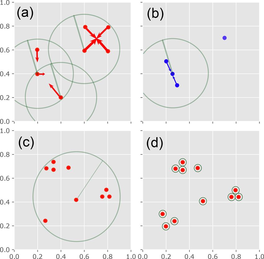
2634                                                                                   M. Mälicke et al.: Soil moisture patterns

   Although large spatial variability seems to be a generic          neous, it is striking how spatially organized they are (Dooge,
feature of soil moisture, there is also evidence that ranks          1986; Sivapalan, 2003; McDonnell et al., 2007; Zehe et al.,
of distributed soil moisture observations are largely stable         2014; Bras, 2015). Spatial organization manifests for in-
in time, as observed at the plot (Rolston et al., 1991; Zehe         stance through systematic and structured patterns of catch-
et al., 2010), hillslope (Brocca et al., 2007, 2009; Blume           ment properties, such as a catena. This might naturally lead
et al., 2009), and even catchment scale (Martínez-Fernández          to a systematic variability of those processes controlling wet-
and Ceballos, 2003; Grayson et al., 1997). This rank stabil-         ting and drying of the soil. One approach to diagnose and
ity, which is also often referred to as temporal stability (Van-     model systematic variability is based on the covariance be-
derlinden et al., 2012), can, i.e., be used to improve sensor        tween observations in relation to their separating distance
networks (e.g., Heathman et al., 2009) or select the most rep-       (Burgess and Webster, 1980) and geostatistical interpolation
resentative observation site in terms of soil moisture dynam-        or simulation methods (Kitanidis and Vomvoris, 1983; Ly
ics (e.g., Teuling et al., 2006). In both cases rank stability       et al., 2011; Pool et al., 2015).
assumes some kind of organization in the catchment, other-              A spatial covariance function describes how linear sta-
wise this representativity would not be observed.                    tistical dependence of observations declines with increasing
   Soil moisture dynamics have been subject to numerous re-          separating distance up to the distance of statistical indepen-
view works (e.g., Daly and Porporato, 2005; Vereecken et al.,        dence. This is often expressed as an experimental variogram.
2008). More specifically, the temporal stability of soil mois-       Geostatistics relies on several assumptions, such as second-
ture was reviewed by Vanderlinden et al. (2012). The authors         order stationarity (see, e.g., Lark, 2012 or Burgess and Web-
analyzed a large number of studies with respect to the con-          ster, 1980), which are ultimately important for interpolation.
trols on time stability of soil water content (TS SWC), yet          Due to the above-mentioned dynamic nature of soil moisture
“the basic question about TS SWC and its controls remain             observations, the most promising avenue for interpolation
unanswered. Moreover, the evidence found in literature with          would be a spatio-temporal geostatistical modeling of our
respect to TS SWC controls remains contradictory” (Vander-           data (Ma, 2002, 2003; De Cesare et al., 2002; Snepvangers
linden et al., 2012, p. 2, l. 2 ff.). We want to contribute by       et al., 2003; Jost et al., 2005).
proposing a method that helps to understand how and when                However, here we take a different avenue, as we do not
spatial soil moisture patterns are persistent.                       intend to interpolate. One of our goals is to detect dynamic
   Soil moisture responds to two main forcing regimes,               changes in the spatial soil moisture pattern. Following Samp-
namely rainfall-driven wetting or radiation-driven drying.           son and Guttorp (1992) we relate the statistical dispersion
The related controlling factors and processes differ strongly        of soil moisture observations to their separating distance to
and operate at different spatial and temporal scales, and the        characterize how their similarity and predictive information
soil moisture pattern reflects thus the multitude of these in-       decline with this distance (see Sect. 2). More specifically,
fluences (Bárdossy and Lehmann, 1998). Hence, we hypoth-             we analyze temporal changes in the spatial dispersion of dis-
esize that periods in which different controlling factors were       tributed soil moisture data and hypothesize that a grouping of
dominant are reflected in fundamentally different soil mois-         the data is possible solely based on the changes in spatial dis-
ture patterns. This can manifest itself in changes in the spatial    persion. We want to find out whether typical patterns emerge
covariance structure (Lark, 2012; Schume et al., 2003), either       in time, how those relate to the different forcing regimes and
in the form of changing nugget-to-sill ratios (spatially ex-         whether those patterns are recurrent in time. The latter is an
plained variance) (Zehe et al., 2010) or state-dependent var-        indicator of predictability and (self-)organization in dynamic
iogram ranges (spatial extent of correlation) (Western et al.,       systems (Wendi and Marwan, 2018; Wendi et al., 2018).
2004). In a homogeneous, flat and non-vegetated landscape               Zehe et al. (2014) argued that spatial organization mani-
the soil moisture pattern shortly after a rainfall event would       fests through a similar hydrological functioning. This is in
be the imprint of the precipitation pattern and provide predic-      line with the idea of Wagener et al. (2007) on catchment
tive information about its spatial covariance. In contrast, in a     classification or the early idea of a geomorphological unit
heterogeneous landscape driven by spatially uniform block            hydrograph (Rodríguez-Iturbe et al., 1979; Sivapalan et al.,
rain events, the spatial pattern of soil moisture would be a         2011; Patil and Stieglitz, 2012). Recently, Loritz et al. (2018)
largely stable imprint of different landscape properties con-        corroborated the idea of Zehe et al. (2014) and showed that
trolling throughfall, infiltration as well as vertical and lateral   hydrological similarity of discharge time series implies that
soil water redistribution. Without further forcing, the spatial      they are redundant. Redundancy in our context means that
pattern will gradually dissipate due to soil water potential de-     new observations (over time) do not add significant new in-
pletion and by lateral soil water flows. We therefore hypothe-       formation to the data set of spatial dispersion. Thus, they can
size that differences in soil moisture (across space) are higher     be compressed without information loss (Weijs et al., 2013).
shortly after a rainfall event and are dissipated afterwards.        This combination of compression rate and information loss
   Landscape heterogeneity is thus a perquisite for temporar-        is understood to be a measure of spatial organization in our
ily persistent spatial patterns found in a set of soil moisture      work. More specifically, Loritz et al. (2018) showed that a
time series. While most catchments are strongly heteroge-            set of 105 hillslope models yielded, despite their strong dif-

Hydrol. Earth Syst. Sci., 24, 2633–2653, 2020                                         https://doi.org/10.5194/hess-24-2633-2020
M. Mälicke et al.: Soil moisture patterns 2635
ferences in topography, a strongly redundant runoff response.
Using Shannon entropy (Shannon, 1948), Loritz et al. (2018)
showed that the ensemble could be compressed to a set of
six to eight typical hillslopes without performance loss. Here
we adopt this idea and investigate the redundancy of patterns
in spatially distributed soil moisture data along with their
compressibility.
The core objective of this study is to provide evidence that
distributed soil moisture time series provide, despite their
strong spatial variability, representative information on soil
moisture dynamics. More specifically, we test the following
hypotheses.
– H1: radiation-driven drying and rainfall-driven wetting
leave different fingerprints in the soil moisture pattern.
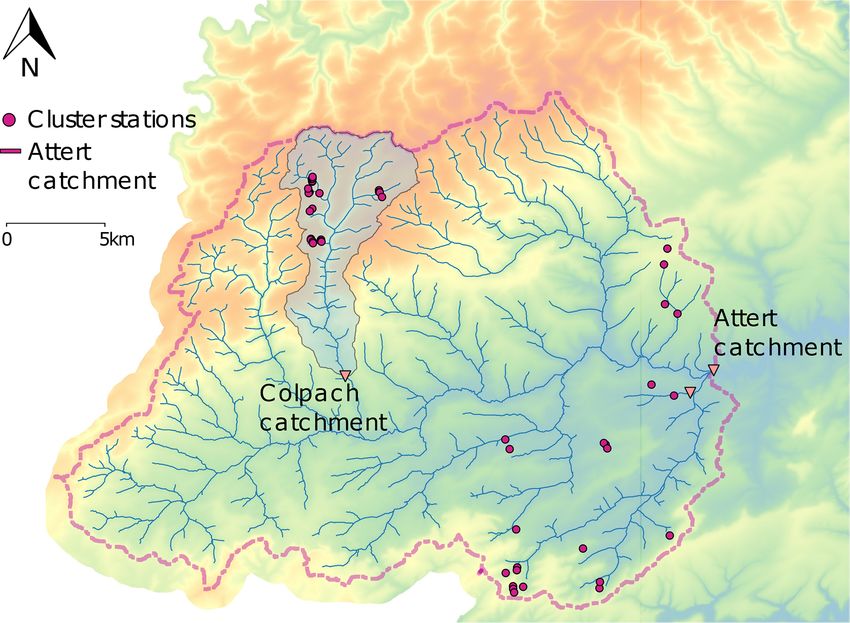
– H2: both forcing regimes and their seasonal variability Figure 1. Attert experimental catchment in Luxembourg and Bel-
may be identified through temporal clustering of disper- gium. The purple dots show the sensor cluster stations installed
sion functions. during the CAOS project. Here we focus on those cluster stations
within the Colpach catchment. Figure adapted after Loritz et al.
– H3: spatial dispersion is more pronounced during and (2017).
shortly after rainfall-driven wetting conditions.
– H4: soil moisture time series are redundant, which im- land use. In the schist area, land use is mainly forest on steep
plies they are compressible without information loss. slopes of the valleys, which intersect plateaus that are used
However, the degree of compressibility is changing over for agriculture and pastures. The marls area has very gentle
time. slopes and is mainly used for pastures and agriculture, while
the sandstone area is forested on steep topography.
We test these hypotheses using a distributed soil moisture
The experimental design is based on spatially distributed,
data set collected in the Colpach catchment in Luxembourg.
clustered point measurements within replicated hillslopes.
In Sect. 2 we give an overview of the study site and our
Typical hillslope lengths vary between 400 and 600 m, show-
method. The results section consists of three parts: spatial
ing maximum elevations of 50 to 100 m above stream level.
dispersion functions, temporal patterns in their emergence
For further details on the hillslopes, we refer the reader to
and some insights into generalization (or compressibility) of
Fig. 6a in Loritz et al. (2017) and a detailed description in
these functions, followed by a discussion and summary.
Sect. 3.1.1 of the same publication. Sensor clusters were in-
stalled on hillslopes at the top, midslope and hill foot sectors
2 Methods along the anticipated flow paths. Within each of those clus-
ters, soil moisture was recorded in three profiles at 10, 30 and
2.1 Study area and soil moisture data set 50 cm depth using Decagon 5TE sensors. While the entire
design was stratified to sample different geological settings
We base our analyses on the CAOS data set, which was col- (schist, marls, sandstone), different aspects and land use (de-
lected in the Attert experimental watershed between 2012 ciduous forest and pasture), we focus here on those sensors
and 2017 and is explained in Zehe et al. (2014). The Attert installed in the Colpach catchment. In total we used 19 sensor
catchment is situated in western Luxembourg and Belgium cluster locations and thus 57 soil moisture profiles consisting
(Fig. 1). Mean monthly temperatures range from 18 ◦ C in of 171 time series.
July to 0 ◦ C in January. Mean annual precipitation is approx- Soil moisture in the 19.4 km2 Colpach catchment exhibits
imately 850 mm (Pfister et al., 2000). The catchment cov- high but temporally persistent spatial variability (Fig. 2). For
ers three geological formations, Devonian schists of the Ar- each point in time a wide range of water content values can
dennes massif in the north-west, a mixture of Triassic sandy be observed across the catchment. The range of soil mois-
marls in the center and a small area on Luxembourg Sand- ture observations is generally wider in winter than in sum-
stone on the southern catchment border (Martinez-Carreras mer. From visual inspection it seems that the heterogeneity
et al., 2012). The respective soils in the three areas are hap- in observations is not purely random but systematic, as the
lic Cambisols in the schist, different types of Stagnosols in measurements are rank stable over long periods. One has to
the marls area and Arenosols in the sandstone (IUSS Work- note that the different cluster locations differ in aspect, slope
ing Group WRB, 2006; Sprenger et al., 2016). The distinct and land use. From the data shown in Fig. 2, two sensors
differences in geology are also reflected in topography and have been removed. Both measured in 50 cm and can be seen
https://doi.org/10.5194/hess-24-2633-2020 Hydrol. Earth Syst. Sci., 24, 2633–2653, 2020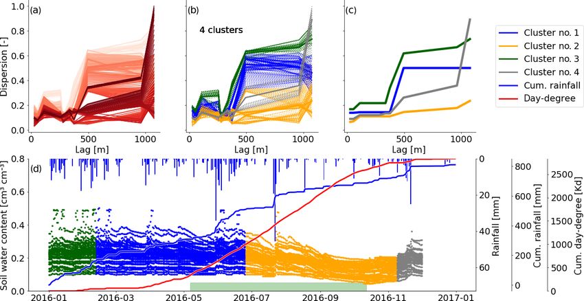
2636                                                                                        M. Mälicke et al.: Soil moisture patterns

Figure 2. Soil moisture data overview. Soil moisture observations in 10 cm (a), 30 cm (b) and 50 cm (c).

in the figure at the very bottom. Both recorded values close to         mean value. Thus, observations taken at a specific distance
or even below 0.1 cm3 cm−3 for the whole period of 4 years.             are more similar in value if they are less dispersed.
Additionally, the plateaus lasting for a couple of days at con-            To estimate the dispersion, we use the Cressie–Hawkins
stant 0.5 cm3 cm−3 in 50 and 30 cm were removed.                        estimator (Cressie and Hawkins, 1980). This estimator is
                                                                        more robust to extreme values and the contained power
2.2    Dispersion of soil moisture observations as a                    transformation handles skewed data better than estimators
       function of their distance                                       based on the arithmetic mean (Bárdossy and Kundzewicz,
                                                                        1990; Cressie and Hawkins, 1980). The estimator is given by
We focus on spatial patterns of soil moisture and how they              Eq. (2):
change over time. For our analysis the data set was aggre-
gated to mean daily soil moisture values θ . Each time series                                                      !4
is further aggregated using a moving window of 1 month as                        1     1 X
                                                                                              q
described by Eq. (1).                                                   at (h) =                |zt (xi ) − zt xj |
                                                                                 2 N (h) i,j
           t+b
                                                                                                      0.045 −1

           P
                 θx                                                                        0.494
            t
                                                                                   0.457 +        + 2            ,                         (2)
zx (t) =                                                       (1)                         N (h) N (h)
                b
This is calculated for each observation location x and time             for each moving window position t with zt (xi,j ) given by
step t = 1, 2, . . . , (L − b), with a time series length of L in       Eq. (1) for each pair of observation locations xi , xj . h is
days and a window size of b = 301 .                                     the separating distance lag between these point pairs and
   To estimate the spatial dependence structure between ob-             N (h) the number of point pairs formed at the given lag h.
servations, we relate their pairwise separation distance to a           Ten classes were formed with a maximum separation dis-
measure of pairwise similarity. Here, we further define the             tance of 1200 m2 . The lag classes are not equidistant, but
statistical spatial dispersion as a measure of spatial similar-         with a fixed N (h) for all classes. This is further discussed
ity. We compare the empirical distribution of pairwise value            in Sect. 2.3.
differences at different distances. Statistically, a more dis-
persed empirical distribution is less well described by its                2 Observation point pairs further apart than 1200 m are most
   1 We tested different window sizes, as we expect that different      likely located on different hillslopes. These points might share simi-
processes control the emergence of spatial dependence at different      lar soil, topographic and terrain aspect characteristics. Soil moisture
temporal scales. The chosen window size was most suitable for de-       dynamics might thus be similar, although they are located at rather
tecting seasonal effects.                                               large separating distances

Hydrol. Earth Syst. Sci., 24, 2633–2653, 2020                                              https://doi.org/10.5194/hess-24-2633-2020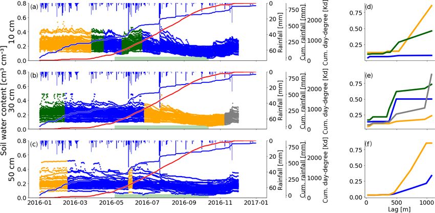
M. Mälicke et al.: Soil moisture patterns                                                                                    2637

2.3   Clustering of dispersion functions                           tonically increasing, they also provide information about the
                                                                   characteristic length of the soil moisture pattern. Similarly to
We analyzed how and whether meaningful spatial disper-             the semi-variogram in geostatistics, this characteristic length
sion functions emerge and whether those converge into stable       corresponds to the lag distance where the dispersion function
configurations. To tackle the hypotheses formulated in the in-     reaches its first local maximum.
troduction, a clustering is applied to the dispersion functions       We suggest that the number of clusters needed to represent
derived for each window. The clustering algorithm should           all observed spatial dispersion functions over a calendar year
form groups of functions that are more similar to each other       can be used as a measure of spatial organization (fewer clus-
than to members of other clusters. The similarity between          ters needed means a higher degree of organization, because
two dispersion functions is calculated by the Euclidean vec-       dispersion functions are redundant in time). Additionally, it is
tor distance between the dispersion values forming the func-       insightful to judge the information loss that goes along with
tion. This distance is defined by Eq. (3):                         this compression, as a high compression with little informa-
           p                                                       tion loss is understood as a manifestation of spatial and tem-
d(u, v) = (u − v)2 ,                                        (3)    poral organization of soil moisture dynamics.
with u, v being two dispersion function vectors. This is the          In line with Loritz et al. (2018) we use the Shannon en-
Euclidean distance of two points in the (higher-dimensional)       tropy as a measure of the compression without information
value space of the dispersion function’s distance lags. Two        loss. It requires treatment of the clusters as discrete proba-
identical dispersion functions are represented by the same         bility density functions, which in turn implies a careful se-
point in this value space, and hence their distance is zero.       lection of an appropriate classification of the data. Motivated
Thus, distance lags are not equidistant, as this could lead        by Loritz et al. (2018), we use the uncertainty in the disper-
to empty lag classes. Empty lag classes result in an unde-         sion function as a minimal class size for this classification,
fined position in the value space, which has to be avoided.        as described in Sect. 2.5.1.
The clustering algorithm cannot use the number of clusters
                                                                   2.5     Uncertainty propagation and compression quality
as a parameter, as this can hardly be determined a priori.
One clustering algorithm meeting these requirements is the         2.5.1    Uncertainty propagation
mean shift algorithm (Fukunaga and Hostetler, 1975). The
actual code implementation is taken from Pedregosa et al.          Soil moisture measurements have a considerable measure-
(2011), which follows the Comaniciu and Meer (2002) vari-          ment uncertainty of 1–3 cm3 cm−3 as reported by manufac-
ant of mean shift. A detailed description of the mean shift        turers. For our uncertainty propagation we assume an abso-
algorithm can be found in the Appendix (see Sect. A).              lute uncertainty/measurement error 1θ of 0.02 cm3 cm−3 .
                                                                      Next we propagate these uncertainties into the dispersion
2.4   Cluster compression based on the cluster centroids           functions and the distances among those. As we assume the
                                                                   measurement uncertainties to be statistically independent, we
The next step is to generate a representative dispersion func-
                                                                   use the Gaussian uncertainty propagation to calculate error
tion for each cluster. The straightforward representative func-
                                                                   bands/margins. In a general form, for any function f (z) and
tion is the cluster centroid (the dispersion function closest to
                                                                   an absolute error 1z the propagated error 1f can be calcu-
the point of highest cluster member density; see Sect. A for a
                                                                   lated. In our case z is itself a function of x, the observation
detailed explanation). All dispersion functions are calculated
                                                                   location, and the general form is given by Eq. (4).
with the same parameters, including the maximum separat-
ing distance of 1200 m. At larger lags we found instances of              v
                                                                          uN                       2
declining dispersion values, because we then paired points
                                                                          uX         ∂f
                                                                   1f = t                   1z (xi )                           (4)
located on different hillslopes but otherwise in similar land-               i=1
                                                                                   ∂z (xi )
scape units (i.e., same hillslope position or land use). To fa-
cilitate the comparison of the dispersion functions we de-         To apply Eq. (4) for our method, the measurement uncer-
cided to monotonize them. In geostatistics this is usually         tainty 1θ is propagated into the dispersion estimator given
done through fitting of a theoretical variogram model to the       by Eq. (2). The dispersion estimator is derived with re-
experimental variogram, which ensures monotony and pos-            spect to z(x) and, following Eq. (1), the uncertainty in z(x),
itive definiteness. Here we do not force a specific shape by       1z, is denoted as 1z = 1θ = 0.02 cm3 cm−3 . Then, with a
a fitting a model function. Instead we use the technique of        given 1z, we can propagate the uncertainty into the disper-
monotonizing the cluster centroid as suggested by Hinterd-         sion function. As the dispersion function is a function of the
ing (2003) using the PAVA algorithm (Barlow et al., 1972).         spatial lag h, we need to propagate the uncertainty 1a (un-
The implementation is from Pedregosa et al. (2011). This           certainty of the dispersion estimator) for each value of h. At
way the final compressed dispersion functions are monoton-         the same time, following Eq. (2), for each h, z(xi ) − z(xi +
ically increasing while still reflecting the shape properties      h) is a fixed set of point pairs. Instead of propagating un-
of the cluster members. If dispersion functions are mono-          certainty through Eq. (2), we can substitute z(xi ) − z(xi + h)

https://doi.org/10.5194/hess-24-2633-2020                                        Hydrol. Earth Syst. Sci., 24, 2633–2653, 2020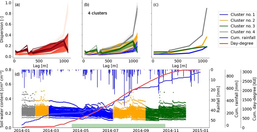
2638                                                                                                    M. Mälicke et al.: Soil moisture patterns

by δ, the pairwise differences, for each value of h. The un-                          of yes/no questions one has to ask to determine the state
certainty 1δ is given by Eq. (5):                                                     of a system. The minimum entropy is zero, which corre-
       q                 √                                                            sponds to the deterministic case where the system state is
1δ = 1zi2 + 1zi+h  2   = 21z.                            (5)                          always known. A common way to define spatial organization
                                                                                      of a physical system is through its distance from the max-
The uncertainty of dispersion 1a is then defined by Eq. (6):                          imum entropy state (Kondepudi and Prigogine, 1998; Klei-
                                                                                      don, 2012). The deviation of the entropy of the dispersion
          ∂a
1a =         1δ                                                                       functions in a cluster from its maximum value is thus a mea-
          ∂δ                                                                          sure of their redundancy and thus similarity.
                                         !3                     ! 12
          1 XN
                        1                       1 XN                                    For a discrete frequency distribution of n bins, the infor-
     = 2c       (|δi |) 2                     ·       |δi |−1          · 1δ,    (6)   mation entropy H is defined as
          N i=1                                 N i=1                                         X
                                                                                      H = − pn log2 (pn ) ,                                     (9)
where the factors from Eq. (2) that stay constant in the deriva-                               n
tive are denoted as c and defined in Eq. (7). In line with
                                                                                      where pn is the relative probability of the nth bin. H is calcu-
Eq. (2) N is the number of observation pairs available for
                                                                                      lated for each depth in each year individually to compare the
a given lag class h and therefore constant for a single calcu-
                                                                                      information content across years and depths. Note that the
lation. 1δ and δ are the substitutes for z, as described above
                                                                                      term bin is also used in the literature to refer to the binning
(see Eq. 5).
                                                                                      of pairwise data, e.g., in geostatistics. For this kind of bin-
      1

                 1  0.045 −1
                                                                                     ning, although technically the same thing, we used the term
c=      · 0.457 + +                                                             (7)   lag classes here to distinguish it from the binning as shown
      2          N   N2
                                                                                      in Eq. (9). Thus, when we write bin or binning we refer to
The last step is to propagate the uncertainty into the distance                       the classification of distances between dispersion functions,
function as defined in Eq. (3). The Euclidean distance is used                        not observation points.
as a measure of proximity by mean shift, as it groups dis-                               To ensure comparability, we use one binning for all cal-
persion functions at short distances together (for more de-                           culations of H (across years and depths). To achieve this, all
tails, see Sect. A). At the same time, we use the uncertainty                         pairwise distances between all spatial dispersion functions of
propagated into the Euclidean distance between two disper-                            all 4 years in all three depths are calculated. The discrete fre-
sion functions to assess compression quality (as further de-                          quency distribution is formed from 0 up to the global maxi-
scribed in Sect. 2.5.2). Following Eq. (4) the propagated un-                         mum distance (between two dispersion functions) calculated
certainty 1d can be calculated by the derivative of Eq. (3)                           using Eq. (3). The bins are formed equidistantly using a
with respect to each of the vectors multiplied by the corre-                          width of the maximum function distance that still lies within
sponding value of 1a, which results in Eq. (8):                                       the error margins calculated using Eq. (8). Thus, the informa-
          s                                                                           tion content of the spatial heterogeneity is calculated with re-
                          2                2

                  ∂d

                                       ∂d                                             spect to the expected uncertainties. This way we can be sure
1du,v =              1u        +          1u
                  ∂u                   ∂u                                             to distinguish exclusively those spatial dispersion functions
 v
 u n
 u1 X               n                                                              that lie outside of the error margins.
                 1 X
=t       |u − v| 2       (2 (|ui − v i |) 1ui )2 + (2 (|ui − v i |) 1v i )2 ,   (8)      The Kullback–Leibler divergence (Kullback and Leibler,
   2 i=1            i=1
                                                                                      1951) is a measure of the difference between two empirical,
where u, v are two spatial dispersion function vectors as de-                         discrete probability distributions. Usually, one distribution is
fined and used in Eq. (3). 1u, 1v are the vectors of uncer-                           considered to be the population and the other one a sample
tainties for u, v, where 1vi is the uncertainty propagated into                       from it. The Kullback–Leibler divergence DKL then quanti-
the ith lag class as shown in Eq. (6). n is the number of lag                         fies the uncertainty introduced (e.g., in an statistical model)
classes and thus the length of each vector u, v, 1u, 1v.                              using a sample as a substitute for the population.
   Equation (8) is applied to all possible combinations of dis-                          We use the Kullback–Leibler divergence to measure and
persion functions u, v to get all possible uncertainties in dis-                      quantify the information loss due to compression. To com-
persion function distances.                                                           press the series of dispersion functions, each cluster member
                                                                                      is expressed by its centroid function. Now, we need to calcu-
2.5.2     Compression quality                                                         late the amount of information lost in this process. To calcu-
                                                                                      late the mean information content of the compressed series,
The Shannon entropy (Shannon, 1948) of all pairwise disper-                           each cluster member is substituted by the respective clus-
sion function distances is used as a measure of information                           ter centroid. This substitution is obviously not a compres-
content. The Shannon entropy of a discrete probability den-                           sion in a technical sense, but it is necessary to calculate the
sity function of states (patterns in this case) is maximized                          Kullback–Leibler divergence. Then a frequency distribution
for the uniform distribution. It corresponds to the number                            for the compressed series X and the uncompressed series Y

Hydrol. Earth Syst. Sci., 24, 2633–2653, 2020                                                          https://doi.org/10.5194/hess-24-2633-2020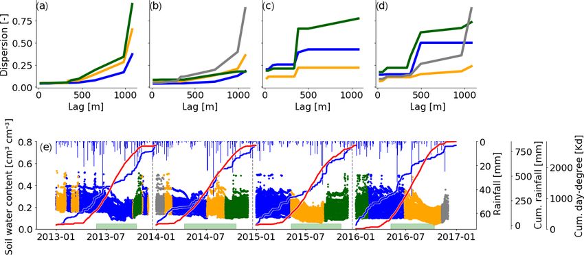
M. Mälicke et al.: Soil moisture patterns 2639
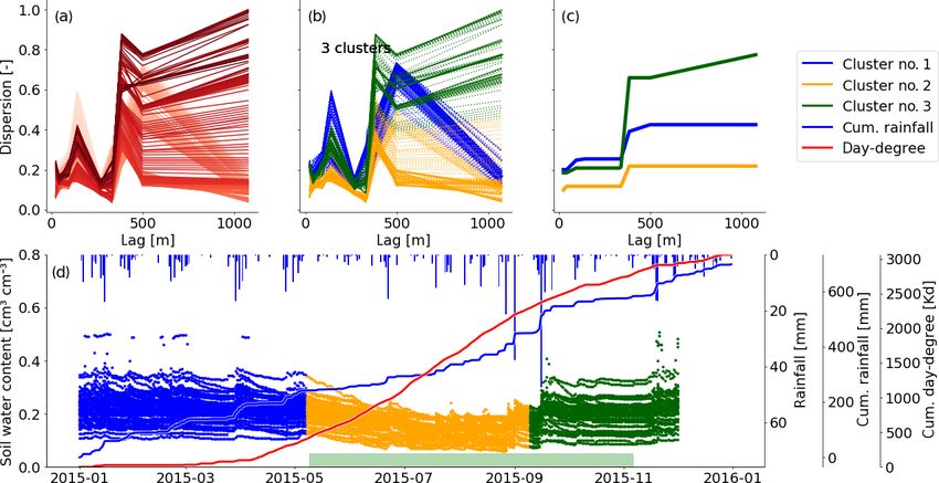
can be calculated. The Kullback–Leibler divergence DKL in Fig. 3c exhibit increasing dispersion with separating dis-
of X, Y is given in Eq. (10): tance. For the blue and green clusters this happens step-
wise at a characteristic distance of 500 m. That reminds us
DKL (X, Y ) = H (X||Y ) − H (Y ), (10) of a Gaussian variogram, which can also show a step-wise
characteristic. The small grey cluster shows an increase at
where H (X||Y ) is the cross entropy of X and Y and defined
500 and another one at 1000 m separating distance. In con-
by Eq. (11):
trast, the orange cluster, however, shows only a gentle in-
X
H (X||Y ) = p(x) · log2 p(y), (11) crease with distance.
x∈X In the vegetation period observations are similar even at
large separating distances. Interestingly, dispersion functions
where p(x) is the empirical non-exceedance probability of in the orange cluster start with small values that only gently
the frequency distribution X and p(y) of Y , respectively. increase with separating distance. That means soil moisture
becomes more homogeneous. Outside of the vegetation pe-
3 Results riod, different spatial patterns can be observed, with increas-
ing dissimilarity with separating distances. The part of the
3.1 Dispersion functions over time blue cluster overlapping with the vegetation period shows
still higher soil moisture values. The transition to the or-
Figure 3a shows the spatial dispersion functions for all mov- ange cluster sets in as the soil moisture drops (Fig. 3d). This
ing window positions in 2016 for the 30 cm sensors. The suggests that vegetation influences, such as root water up-
position of the moving window in time can be retraced by take, smooth out variability in soil water content, leading to
the line color: darker red means a later Julian day. Each of a more homogeneous pattern in space, as further discussed in
the spatial dispersion functions relates the dispersion for all Sect. 4.3.
pairwise observations to their separating distance in the cor-
responding lag class. Dispersion increases with separating 3.2 Dispersion time series as a function of depth
distance, as small values correspond to observations which
have similar values, while large values suggest the opposite. Figure 4 shows the time series of the dispersion functions for
As expected, the dispersion is a suitable metric for similar- all depths. Note that the coloring between the sub-figure is
ity/dependency of observations. arbitrary, due to mean shift, which means there is no connec-
The spatial dispersion functions take several distinct tion between the orange cluster between the three figures.
shapes, with each of these shapes occurring during a cer- In comparison to the dispersion functions in 30 cm
tain period in time. More specifically, from Fig. 3a one can (Fig. 4b) the soil moisture signal in 10 cm (Fig. 4a) is more
identify groups of functions of similar reds plotting close to variable in time. A look at the centroid of the orange clus-
each other. Dispersion functions of similar red saturation, ter (Fig. 4d) reveals a higher spatial heterogeneity in winter
which reflects proximity in time, are also similar in shape, and spring at large separating distances. At the same time
and this in turn reflects similar spatial patterns. Similar dis- the observations get spatially more homogeneous in summer,
persion functions were grouped using the mean shift cluster- particularly when the blue cluster emerges; i.e., the disper-
ing algorithm (Fig. 3b); here, the color indicates the cluster sion at large lags decreases significantly. We can still find
membership. a summer-recession cluster in 10 cm, but compared to the
To provide further insight into the temporal occurrence of depth of 30 cm we also find this spatial footprint of continu-
cluster members, we colored the soil moisture time series ac- ous drying earlier in the year around May. This is likely due
cording to the color codes of the identified clusters (Fig. 3d). to a higher sensitivity to rising temperatures. Note that dur-
The blue parts of the soil moisture time series were classi- ing May there was only little rainfall and the soil moisture is
fied into Cluster no. 1, while the orange part was classified already declining. This blue cluster shows very small disper-
into Cluster no. 2. Note that cluster memberships are constant sion values for all separating distance classes (Fig. 4d), just
for long periods of time, which means that the soil moisture as the orange cluster in 30 cm depth.
patterns are also persistent over these periods. Exact cluster The green clusters emerge with strong rainfall events after
lifespans can be found in Table B1. We could identify four longer previous dry spells (Fig. 4a and d). We would have ex-
clusters in 30 cm, with the orange cluster roughly occurring pected a third occurrence at the beginning of August, but the
during the vegetation period and the other three the remain- soil may already be too dry to bear a detectable dependency
ing time of the year. As new observations did not change the on separating distance (remember that the blue cluster does
patterns during these periods, they were redundant in time. not show increasing dispersion with distance).
As the spatial dispersion functions in the presented exam- Observations at 50 cm depth show a clear spatial depen-
ple are redundant in time, we compressed the information dency throughout the whole year. We cannot identify a sum-
by replacing the dispersion function within one cluster by mer cluster, mean shift yielded two clusters and rainfall forc-
the cluster centroid. All four representative functions shown ing does not have a clear influence on their occurrence or
https://doi.org/10.5194/hess-24-2633-2020 Hydrol. Earth Syst. Sci., 24, 2633–2653, 20202640 M. Mälicke et al.: Soil moisture patterns Figure 3. Spatial dispersion functions in 30 cm for 2016 based on a window size of 30 d. (a) Spatial dispersion function for each position of the moving window. The red color saturation indicates the window position. The darker the red, the later in the year. (b) The same dispersion functions as presented in (a). Here the color indicates cluster membership as identified by the mean shift algorithm. (c) Compressed spatial dispersion information represented by corrected cluster centroids. The colors match the clusters as presented in (b). (d) Soil moisture time series of 2016 in 30 cm depth. The colors identify the cluster membership of the spatial dispersion function of the current window location and match the colors in (b) and (c). The bars on the top show the daily precipitation sums. The solid blue line is the cumulative daily precipitation sum and the red line the cumulative sum of all mean daily temperatures > 5 ◦ C. The green bar marks the assumed vegetation period. It covers the dates where the cumulative day-degree sum is > 15 % and < 90 % of the maximum. Figure 4. Soil moisture time series of 2016 in all three depths with respective cluster centroids. The three rows show the data from 10 cm (a), 30 cm (b) and 50 cm (c). The colors indicate the cluster membership of the corresponding dispersion function of the respective window position. The green bar marks the assumed vegetation period. It covers the dates where the cumulative day-degree sum is > 15 % and < 90 % of the maximum. The cluster centroids for each depth are shown in (d–f). Hydrol. Earth Syst. Sci., 24, 2633–2653, 2020 https://doi.org/10.5194/hess-24-2633-2020
M. Mälicke et al.: Soil moisture patterns                                                                                        2641

transition. The two 50 cm dispersion functions (Fig. 4f) show    Table 1. Qualitative description of method success in all years and
a clear dependence on distance, but they differ in their dis-    depths. The results from years other than 2016 and all depths were
persion value at large lags. At 10 and 30 cm we found dis-       inspected visually and are summarized here for the sake of com-
persion functions of fundamentally different shapes, like the    pleteness. The first three columns identify the year, sensor depth
flat, blue function (Fig. 4,d) or the step-wise blue and green   and number of clusters found by mean shift. The remaining three
                                                                 columns state whether specific features existed in the given result.
functions (Fig. 4e). At 50 cm depth the characteristic length
                                                                 Vegetation period marks whether or not the vegetation period was
is 500 m and the blue cluster persists throughout most of the    characterized by a single, or two, clusters. Spatial structure: does a
year (282 d; see Table B1). The orange cluster occurs during     dependency of dispersion on distance exist outside the vegetation
the cool and wet start of the year, showing a larger disper-     period? Rainfall transition: were cluster transitions accompanied
sion and thus stronger dissimilarity at larger lags (Fig. 4f).   by a rainfall event in close (temporal) proximity? This feature is
Interestingly this cluster occurs again in early June after an   marked “yes” if it was more often the case than it was not.
intense rainfall period. However, a similar rainfall period in
August does not trigger the emergence of this orange cluster      Year     Depth      No. of    Vegetation    Spatial     Rainfall
as the topsoil above 50 cm is so dry, so that even this strong                       clusters   period        structure   transition
wetting signal does not reach the depth of 50 cm (Fig. 4c).       2013       10         4       yes           no          no
This behavior reveals the low-pass behavior of the topsoil,       2013       30         3       no            yes         yes
which causes a strong decoupling of the soil moisture pat-        2013       50         6       no            yes         yes
tern at 50 cm depth from event-scale changes.                     2014       10         3       yes           no          yes
                                                                  2014       30         4       no            yes         no
3.3   Recurring spatial dispersion over the years                 2014       50         5       no            yes         yes
                                                                  2015       10         3       yes           yes         no
                                                                  2015       30         3       yes           yes         yes
Table 1 summarizes the most important features of the clus-
                                                                  2015       50         3       no            yes         no
tering for all observation depths. Soil moisture patterns and
                                                                  2016       10         3       no            yes         yes
their clustering appear generally to be clearer for 2015          2016       30         4       yes           yes         yes
and 2016. The vegetation period is more often character-          2016       50         2       no            yes         no
ized by a typical cluster and dispersion functions more of-
ten reveal a clear spatial dependency. In some cases (10 cm,
2013 and 2014) no spatial dependency of dispersion func-
tions could be observed throughout the whole year. Less clus-    the division into calendar years is rather meaningless, while
ters were formed in 2015 and 2016. Note that annual rain-        the division into hydrological years is much more appropri-
fall sums were higher in 2013 and 2014, while 2015 and           ate, as is reflected by the cluster membership and its changes.
2016 had significantly more precipitation in the first half          Distinct summer recessions in soil moisture are only iden-
of the year, followed by a dry summer (compared to 2013          tified in 2015 and 2016. Evapotranspiration (indicated by the
and 2014).                                                       cumulative temperature curves in Fig. 5e) dominates over
   To further illuminate interannual changes in soil moisture    rainfall input (blue sum curve) in the soil moisture signal.
patterns, we present the time series of cluster memberships      Mean shift could identify a significantly distinct spatial de-
for the sensors in 30 cm for the entire monitoring period        pendency in dispersion, as shown by the two orange centroids
in Fig. 5. From this example it becomes obvious that pat-        in Fig. 5c and d. They are both distinct from the other cen-
terns are recurring. Years 2013 and 2014 cluster centroids       troids in the same period by showing only a gentle increase in
look different from the following 2 years. Dispersion val-       dispersion. A likely reason for the absence of a distinct sum-
ues increase with distance in all centroids in 2013 and 2014,    mer recession in 2014 is the rather wet and cold spring and
while 2015 and 2016 show a sudden increase at 400–500 m          summer, as can be seen from the steep cumulative rainfall
(Fig. 5a–d). Years 2015 and 2016 are segmented by mean           curve during that period (Fig. 5e). In 2013 this identification
shift in a similar way, and cluster centroids reveal that the    did not work. Possible reasons are provided in the discussion
green clusters in both years are actually the same. This green   Sect. 4.5.
cluster emerges with the occurrence of the largest rainfall
event in the observation period and lasts for around 5 months.   3.4   Redundant spatial dispersion functions
All dispersion functions within this cluster look nearly iden-
tical (see Fig. C2b). Similar observations can be made be-       We calculated the Shannon entropy for all soil moisture time
tween 2014 and 2015. Here, the green and blue clusters           series for all years and depths (Table 2). As explained in
seem to be an interannual cluster. However, in contrast to       Sect. 2.5.2 this reflects the intrinsic uncertainty of the clus-
2015/2016, the dispersion functions here are of a different      ters. Most entropy values are within a range of 1 < H < 2.5.
shape (see Fig. C1b). Hence, the cluster transition indicated    The maximum possible entropy for a uniform distribution
between 2014 and 2015 is indeed a real transition. When          of the used binning is 3.55. The Kullback–Leibler diver-
looking at cluster memberships throughout the whole period,      gence DKL is a measure of the information loss due to the

https://doi.org/10.5194/hess-24-2633-2020                                      Hydrol. Earth Syst. Sci., 24, 2633–2653, 2020
2642 M. Mälicke et al.: Soil moisture patterns
Figure 5. Soil moisture time series of all years in 30 cm depth (e) and the respective cluster centroids (a–d). The colors of the soil moisture
data indicate the cluster membership of the corresponding dispersion function of the respective window position and correspond to the color
of the cluster centroid (in a–d). The cumulative rainfalls (blue) and cumulative temperature sums (red) are shown for each year individually.
The green bar marks the assumed vegetation period. It covers the dates where the cumulative day-degree sum is > 15 % and < 90 % of the
maximum.
Table 2. Information content and information loss due to com- than one-third in almost all cases (2016; 50 cm is the only
pression. The information content is given as Shannon entropy H , exception). In the majority of the cases it does not contribute
which is the expectation value of information in information the- more than 20 %.
ory. 2H gives the number of distinct states the underlying distribu- According to Eq. (9) the Shannon entropy is derived from
tion can resolve. The information loss after compression is given a discrete, empirical probability distribution. As it is calcu-
by the Kullback–Leibler divergence DKL between the compressed
lated using the binary logarithm, 2H gives the amount of dis-
and uncompressed series of dispersion functions. The last column
relates DKL to H .
criminable states in this discrete distribution. This number
of states is deemed to be a reasonable upper limit for the
Year Depth No. of H 2H DKL DKL · (H + DKL )−1 number of clusters for mean shift. A higher number of clus-
clusters (bit) (bit) ters than 2H appears meaningless, and this ensures that only
2013 10 cm 4 0.97 1.95 0.44 0.31 those clusters are separated which are separated by a distance
2013 30 cm 3 1.49 2.81 0.06 0.04 larger than the margin of uncertainty.
2013 50 cm 6 2.0 3.99 0.13 0.06
2014 10 cm 3 1.35 2.55 0.22 0.14
2014 30 cm 4 1.57 2.97 0.3 0.16
2014 50 cm 5 2.44 5.42 0.28 0.1 4 Discussion
2015 10 cm 3 1.87 3.67 0.18 0.09
2015 30 cm 3 1.18 2.26 0.09 0.07 In line with our central hypothesis H1 – that radiation-driven
2015 50 cm 3 2.39 5.24 0.9 0.27
2016 10 cm 3 2.49 5.62 0.76 0.23 drying and rainfall-driven wetting leave different fingerprints
2016 30 cm 4 1.44 2.71 0.02 0.02 in the soil moisture pattern which manifests in temporal
2016 50 cm 2 3.21 9.27 2.5 0.44 changes in the dispersion functions – we found strong ev-
idence that soil water dynamics is organized in space and
time. Our findings reveal that this organization is not static
compression of the cluster onto the centroid dispersion func- but exhibits dynamic changes which are closely related to
tion. In the overwhelming majority of the cases, the informa- seasonal changes in forcing regimes. A direct consequence is
tion loss is 1 magnitude smaller than the intrinsic uncertainty that soil moisture observations are quite predictable in time
and the range is 0.01 < DKL < 0.4. Hence, the information despite their strong spatial heterogeneity. This is in line with
loss due to compression is negligible. There is one exception conclusions of, e.g., Mittelbach and Seneviratne (2012) or
in 2016 (50 cm). Teuling et al. (2006), who also found characteristic spatial
The clusters obtained in 30 cm for the year 2016 (compare patterns to persist in time. We used the statistical dispersion
Sect. 3.1) showed an entropy of 1.44. Compared to this value, of soil moisture observations in dependence of their separat-
the Kullback–Leibler divergence caused by compression of ing distance to describe spatial patterns. The vector distance
only 0.02 is small, if not negligible. The last column of Ta- of these dispersion functions was used to cluster them. As a
ble 2 relates DKL to the overall uncertainty. It contributes less measure of the degree of organization we used the informa-
Hydrol. Earth Syst. Sci., 24, 2633–2653, 2020 https://doi.org/10.5194/hess-24-2633-2020M. Mälicke et al.: Soil moisture patterns 2643
tion loss that goes along with the compression of the entire dissimilarity at larger distances and that pattern lasted for
cluster, i.e., the replacement of the cluster by the most repre- a couple of weeks. Then, evapotranspiration-driven drying
sentative cluster member. Here we found that this compres- smooths out soil moisture variability and during a similarly
sion adds negligible uncertainty compared to the intrinsic un- strong rainfall event in summer, the cluster can not emerge
certainty, caused by propagation of measurement uncertain- again as the soil is already too dry. The soil acts as a low-
ties. We thus conclude that soil moisture is heterogeneous but pass filter here, which filters out any change in state above
temporally persistent over several months. a specific frequency. This happens mainly due to dispersion
In the following we will discuss our main findings that of the infiltrating and percolating water through the soil, or
similarity in space leads to dynamic similarity in time, the due to storage in the soil matrix. By the time it reaches the
way we utilized the measurement uncertainty to determine deep layers, spatial differences are eliminated. This kind of
the information content and how two different processes behaviour is well known and was already reported in the
forcing soil moisture dynamics induce two fundamentally early 1990s (Entekhabi et al., 1992; Wu et al., 2002). More
different spatial patterns. recently Rosenbaum et al. (2012) “found large variations in
spatial soil moisture patterns in the topsoil, mostly related
4.1 Spatial similarity persists in time to meteorological forcing. In the subsoil, temporal dynamics
were diminished due to soil water redistribution processes
We related the dispersion of pairwise point observations to and root water uptake”. In the same year, Takagi and Lin
their separating distance. For brevity and due to their shape (2012) analyzed a data set of 106 locations in a forested
we called these relationships dispersion functions. We em- catchment in the US for spatial organization in soil mois-
phasize that this term is not meant in a strict sense, and no ture patterns. They found a seasonal change in more shallow
mathematical functional relationship, analogous to a theo- depths (30 cm), controlled by rainfall and evapotranspiration.
retical model, has been fitted to the experimental dispersion In deeper depths patterns became more temporally persistent.
functions. Despite the fact that the presented functions are All these findings are in line with our results and conclusions.
empirical, they show clear, recurrent shapes on many occa- Mittelbach and Seneviratne (2012) decomposed a long-
sions. term (15-month) soil moisture time series into time-invariant
We found spatial similarity to persist in time. This is re- and dynamic contributions to the spatial variance. Their data
flected in the temporal stability in cluster membership. In line set spanned 14 sites from Switzerland at a clearly different
with H2 – that both forcing regimes and their seasonal vari- scale (150×210 km). The study quantified the time-invariant
ability may be identified through temporal clustering of dis- contribution on average to 94 %, which leads to “a smaller
persion functions – the results (Figs. 3–5) provided evidence spatial variability of the temporal dynamics than possibly in-
that similar dispersion functions emerge in fact very closely ferred from the spatial variability of the mean soil moisture”
in time. Generally they appeared in continuous periods or (Mittelbach and Seneviratne, 2012, p. 2177, l. 14 ff.). This is
blocks in time and their changes coincided with changes or a comparable to the instances where we find long-lasting clus-
switch in the forcing regimes. In case we can relate the emer- ters, while the absolute soil moisture changes considerably
gence of such a cluster more quantitatively to the nature and (e.g., Fig. 3d), early April or mid-July).
strength of a specific forcing event/process, we can analyze
for how long this event/process imprints the spatial pattern 4.2 Uncertainty analysis
of soil moisture observations. Or in other words: we can an-
alyze how long a catchment state remembers a disturbance. We related the evaluation of compression quality directly to
However, an attempt to relate cluster transitions to rainfall the measurement uncertainty. This was achieved by Gaus-
sums and frequencies within the respective moving windows sian error propagation of measurement uncertainty into the
(see Fig. B1) did not yield clear dependencies. dispersion functions and their distances. The latter allowed
Although cluster memberships occur in temporally con- definition of a minimum separable vector distance between
tinuous blocks in all depths throughout all years, for a few two dispersion functions that are different with respect to
cases we could not relate their emergence to distinct changes the error margin. We based the bin width for calculating the
in forcing. This implies that H2 needs to be partly revised. Shannon entropy on this minimum distance, because this en-
Dispersion functions in 50 cm show a clear spatial depen- sured that the Shannon entropy gives the information content
dency throughout the year, with distinct differences within of each cluster with respect to the uncertainty. On this basis
and outside the vegetation period. In 50 cm of 2016 this is it was possible to assess compression quality not only by the
different. We find essentially two clusters that do not sepa- number of meaningful clusters found, but also based on the
rate the data series by vegetation period. The shape of the two information lost due to compression with respect to uncer-
centroids (Fig. 4f) is similar, only at large distances they dif- tainty.
fer in value. This means that from the orange to blue clusters In line with H4, spatial patterns of soil moisture were
observations became more similar at large separating dis- found to be persistent over weeks, if not months. In many
tances. Heavy rainfall disturbs this pattern leading to stronger instances we found only two to four clusters within 1 year,
https://doi.org/10.5194/hess-24-2633-2020 Hydrol. Earth Syst. Sci., 24, 2633–2653, 20202644 M. Mälicke et al.: Soil moisture patterns
and compression was possible with small if not negligible hillslope length for the Colpach catchment. During the veg-
information loss. That means that during one cluster period etation period variability at a large separating distance was
an entire set of dispersion functions does not contain substan- smoothed out. Dispersion was low also at large distances,
tially more information than the centroid function. Hence, the suggesting similarity even at distances larger than the typi-
whole cluster can be represented by only the centroid func- cal slope length. We thus conclude that there is dependence
tion. We conclude that this is a manifestation of a strongly or- of the dispersion on the rainfall pattern, which is reflected
ganized state which persists for a considerable time, as most in the dispersion function’s shape and characteristic length.
observations were redundant during these periods. This confirms H2 and suggests that vegetation is a possible
Teuling et al. (2006) concluded that picking a random soil dominant factor in smoothing out soil moisture variability.
moisture observation location and deriving the temporal dy- A similar conclusion is drawn by Meyles et al. (2003), who
namics from this single sensor is more accurate than using identified “preferred states in soil moisture” (Grayson et al.,
the spatial mean of many soil moisture time series. This con- 1997; Western and Grayson, 1998; Western et al., 1999) and
clusion was true for all three data sets they tested (Teuling could relate the state transition to a significant change in the
et al., 2006). This representativity of a single sensor to our characteristic length of their geostatistical analysis. We gen-
understanding is a manifestation of a persistent spatial pat- erally found more than two clusters, but we still consider
tern in soil moisture dynamics, which also enables us to com- these results to be comparable. Most of the clusters identified
press clusters without information loss. during the vegetation period are more similar to each other
From Eq. (9) it can be seen that the Shannon entropy than to the clusters outside of the vegetation period (and vice
changes substantially with the binning. Therefore, it is of versa). This can be related to the “wet” and “dry” states in
crucial importance to define a meaningful binning based Meyles et al. (2003). Although conducted in a very different
on objective criteria. We suggest that only a discrimination climate, McNamara et al. (2005) also widened the separation
into bins larger than the error margins makes sense, because of two preferred states into five, which they found to be ex-
smaller differences cannot be resolved based on the precision planatory for runoff generation. Interestingly they found the
of the sensors. For the application presented in this work, seasonal interplay of precipitation and evapotranspiration re-
this is important because otherwise one could not compare sponsible for transitions between states. Vanderlinden et al.
the compression quality between depths or years, as different (2012) further reference Gómez-Plaza et al. (2001) as an ex-
binnings lead to different Shannon entropy values, even for ample study, which identified vegetation as the dominant fac-
the same data. Hence, it would be difficult to analyze effects tor. Plant root activity is changing the temporal stability of
or differences of spatial dispersion in depth or over the years. soil moisture in the upper 20 cm of the soil considerably.
We thus conclude that the Shannon entropy should only be Outside the vegetation period we observed multiple clus-
used if the measurement uncertainties of the data are prop- ter transitions. Although more than one cluster was identi-
erly propagated. fied, the clusters were more similar in shape to each other
We provided an example of how the quality of a compres- than to the clusters in the “dry” summer period. In many
sion can be assessed. Instead of considering the number of cases these cluster transitions coincided with a shift in rain-
clusters (compression rate) only, we linked the compression fall regimes. Either the first stronger rainfall event after a
rate to the resulting information loss. We could show that in longer period without rainfall sets in, or one of the heav-
the majority of the cases substantial compression rates could iest rainfall events of that year occurs. There are also in-
be achieved, which are accompanied by negligible informa- stances with recurring clusters that develop more than once
tion losses. We thus suggest that the trade-off between com- (e.g., Figs. 3, 4a, c and 5e). As these periods are controlled by
pression rate and information loss should be used as a com- rainfall, either different rainfall patterns or different hydro-
pression quality measure. logical processes are dominating. Depending on antecedent
wetness, rainfall amounts and rainfall intensity, infiltration
4.3 Different dominant processes lead to different and subsurface flow processes can change and thus also al-
patterns ter the soil moisture pattern. Although this may only be a
coincidence, we found the green cluster in 2016 (Fig. 3) to
Outside of the vegetation period, we found a recurring pic- form with strong rainfall input setting in after a period of lit-
ture of spatial dispersion functions with characteristic lengths tle rainfall. Similar observations can be made for other years,
clearly smaller than the typical extent of hillslopes. Disper- unfortunately not in all cases. Consequently, we can neither
sion functions were calculated in three depths for every day confirm nor reject H3 – that spatial dispersion is more pro-
throughout 4 years. In most cases there is an characteris- nounced during and shortly after rainfall-driven wetting con-
tic length at which the dispersion function shows a sudden ditions.
rise in dispersion. For spatial lags smaller than this distance Many other works also tried to link soil moisture pattern
the dispersion is usually very small. Higher lags show much to forcing. Teuling and Troch (2005) report for soil moisture
higher and more variable dispersion values. This character- measurements taken on an agricultural field in Belgium that
istic length is approx. 500 m. This corresponds to a common the first rainfall events in the late growing season even out the
Hydrol. Earth Syst. Sci., 24, 2633–2653, 2020 https://doi.org/10.5194/hess-24-2633-2020You can also read