Contrasting seismic risk for Santiago, Chile, from near-field and distant earthquake sources
←
→
Page content transcription
If your browser does not render page correctly, please read the page content below
Nat. Hazards Earth Syst. Sci., 20, 1533–1555, 2020
https://doi.org/10.5194/nhess-20-1533-2020
© Author(s) 2020. This work is distributed under
the Creative Commons Attribution 4.0 License.

Contrasting seismic risk for Santiago, Chile, from near-field
and distant earthquake sources
Ekbal Hussain1,2 , John R. Elliott1 , Vitor Silva3 , Mabé Vilar-Vega3 , and Deborah Kane4
1 COMET,  School of Earth and Environment, University of Leeds, Leeds, LS2 9JT, UK
2 British
        Geological Survey, Natural Environment Research Council, Environmental Science Centre,
Keyworth, Nottingham, NG12 5GG, UK
3 GEM Foundation, Via Ferrata 1, 27100 Pavia, Italy
4 Risk Management Solutions, Inc., Newark, CA, USA

Correspondence: Ekbal Hussain (ekhuss@bgs.ac.uk)

Received: 1 February 2019 – Discussion started: 11 March 2019
Revised: 20 March 2020 – Accepted: 29 March 2020 – Published: 29 May 2020

Abstract. More than half of all the people in the world now         districts, such as Ñuñoa, Santiago, and Providencia, where
live in dense urban centres. The rapid expansion of cities,         targeted retrofitting campaigns would be most effective at
particularly in low-income nations, has enabled the eco-            reducing potential economic and human losses. Due to the
nomic and social development of millions of people. How-            potency of near-field earthquake sources demonstrated here,
ever, many of these cities are located near active tectonic         our work highlights the importance of also identifying and
faults that have not produced an earthquake in recent mem-          considering proximal minor active faults for cities in seismic
ory, raising the risk of losing hard-earned progress through a      zones globally in addition to the more major and distant large
devastating earthquake. In this paper we explore the possible       fault zones that are typically focussed on in the assessment
impact that earthquakes can have on the city of Santiago in         of hazard.
Chile from various potential near-field and distant earthquake
sources. We use high-resolution stereo satellite imagery and
imagery-derived digital elevation models to accurately map          1   Introduction
the trace of the San Ramón Fault, a recently recognised ac-
tive fault located along the eastern margins of the city. We        Earthquakes are caused by the sudden release of accumu-
use scenario-based seismic-risk analysis to compare and con-        lated tectonic strain that increases in the crust over decades
trast the estimated damage and losses to the city from several      to millennia. Many faults are often not recognised as danger-
potential earthquake sources and one past event, comprising         ous because they have not recorded an earthquake in living
(i) rupture of the San Ramón Fault, (ii) a hypothesised buried      and written memory (e.g. England and Jackson, 2011). Since
shallow fault beneath the centre of the city, (iii) a deep intra-   probabilistic seismic-hazard assessments (PSHAs) rely on
slab fault, and (iv) the 2010 Mw 8.8 Maule earthquake. We           knowledge of past seismicity to determine hazard levels, the
find that there is a strong magnitude–distance trade-off in         regions around these faults are often deemed to be low haz-
terms of damage and losses to the city, with smaller magni-         ard in seismic-risk assessments until an earthquake strikes
tude earthquakes in the magnitude range of 6–7.5 on more            and the assessment is revised (Stein et al., 2012). The 2010
local faults producing 9 to 17 times more damage to the             Mw 7.0 Haiti earthquake, with its close proximity to an urban
city and estimated fatalities compared to the great magnitude       centre, was a stark reminder of how ruptures on these faults
8+ earthquakes located offshore in the subduction zone. Our         can be so deadly, especially when they are located near ma-
calculations for this part of Chile show that unreinforced-         jor population centres in poorly prepared low-income nations
masonry structures are the most vulnerable to these types           (Bilham, 2010).
of earthquake shaking. We identify particularly vulnerable

Published by Copernicus Publications on behalf of the European Geosciences Union.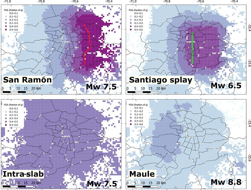
1534 E. Hussain et al.: Seismic risk in Santiago
The South American country of Chile is one of the most
seismically active countries in the world. Since 1900 there
have been 11 great earthquakes in the country with magni-
tudes 8 or larger (USGS, 2019). All of these were located
on or near the subduction interface where the Nazca plate is
subducting beneath the South American plate at 7.5 cm yr−1
(DeMets et al., 2010), giving rise to the Andean mountain
range (Armijo et al., 2015; Oncken et al., 2006). It is there-
fore unsurprising that shaking from offshore subduction zone
events dominates the seismic hazard – thus the building de-
sign – criteria in Chile (e.g. Fischer et al., 2002; Pina et al.,
2012; Santos et al., 2012). The most recent great event was
the Mw 8.8 Maule earthquake, which struck southern Chile in
2010, generating a tsunami and causing 521 fatalities. How-
ever, large, shallow-crustal (< 15 km depth) earthquakes are
not uncommon in Chile. Since 1900 there have been nine
magnitude 7+ shallow-crustal earthquakes located inland
and therefore not directly associated with slip on the sub-
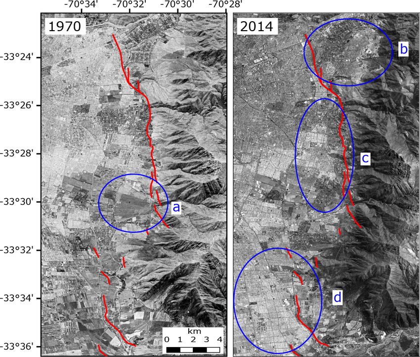
duction megathrust (USGS, 2019). But most of these faults Figure 1. Declassified corona satellite image (∼ 2 m resolution)
accumulate strain at slower rates compared to the subducting from 1970 (left) and the same region in the SPOT imagery (1.5 m
plate boundary and thus rupture infrequently. resolution; right) used in this study showing the eastward expan-
The San Ramón Fault is one such fault. It runs along sion of the city over the San Ramón Fault (red lines). Four notable
the foothills of the San Ramón mountains and bounds the regions are highlighted in blue: (a) an alluvial fan that is clearly
eastern margin of the capital city Santiago, a conurbation visible in the older imagery but completely covered with buildings
in the recent image, (b) expansion into the foothills of the moun-
which hosts 40 % of the country’s population within the
tain and onto the hanging wall of the San Ramón thrust fault (these
city’s metropolitan region (7 million according to 2017 es-
are often more affluent neighbourhoods with better views across the
timates). Due to the rapid expansion of the city in the 20th city), (c) urban densification in the central regions, and (d) land use
and 21st centuries (Ramón, 1992), parts of the fault now lie change from farmland to dense urban neighbourhood masking the
beneath the eastern communes (districts) of the city (Fig. 1), fault trace.
in particular Puente Alto, La Florida, Peñalolén, La Reina,
and Las Condes. Yet it was only as recent as the past decade
that Armijo et al. (2010) recognised that the San Ramón which is compatible with the earlier estimates by Armijo
Fault is an active Quaternary thrust fault and poses a sig- et al. (2010) and the recurrence slip rates deduced from
nificant hazard to the city. Using field mapping and satel- the palaeo-earthquakes in the trench study by Vargas et al.
lite imagery they estimated a slip rate of ∼ 0.5 mm yr−1 for (2014). This suggests that most of the active deformation
the fault, a much slower loading rate compared to the overall across the West Andean fold-and-thrust belt is accommo-
7.5 cm yr−1 plate convergence rate in the subduction zone. dated on the San Ramón Fault. Therefore, despite the very
Palaeo-seismic trench studies across the San Ramón Fault low slip rates, the long time interval since the last earthquake
scarp revealed records of two historical ∼ 5 m slip events – means that significant strain has now accumulated on the
approximately equivalent to a pair of Mw 7.5 earthquakes – fault, and if it were to rupture completely, it could produce
17–19 and ∼ 8 kyr ago (Vargas et al., 2014). However, based earthquakes of an equivalent magnitude as those recorded in
on geophysical investigations of the fault region, Estay et al. the trench.
(2016) concluded that the San Ramón Fault is segmented into Pérez et al. (2014) performed a detailed analysis of local
four sub-faults that are most likely activated independently in seismicity for the region and showed that the microseismic-
earthquakes with moment magnitude in the range of 6.2 and ity at depth (∼ 10 km) can be associated with the San Ramón
6.7. While Estay et al. (2016) do not discount the possibil- Fault, implying that the fault is indeed active and accumulat-
ity of a larger rupture linking across all four segments, evi- ing strain. Vaziri et al. (2012) used Risk Management Solu-
dence from the trench studies (Vargas et al., 2014) suggests tions’ (RMS) commercial catastrophe risk modelling frame-
that larger-magnitude earthquakes are possible on the fault. work to estimate the losses from future earthquakes on the
Therefore for the seismic hazard and risk analysis in this pa- San Ramón Fault for Santiago. They estimate that a Mw 6.8
per we take the worst-case scenario of a complete rupture earthquake on the fault could result in 14 000 fatalities with a
along the fault as our scenario case study. building loss ratio of 6.5 %. However, the spatial distribution
Riesner et al. (2017) used balanced kinematic reconstruc- of these losses remains unclear.
tions of the geology across the region to deduce a long-term Building on this previous work of identifying the hazard
average shortening rate of between 0.3 and 0.5 mm yr−1 , and losses, we aim to contrast the risk posed by the San
Nat. Hazards Earth Syst. Sci., 20, 1533–1555, 2020 https://doi.org/10.5194/nhess-20-1533-2020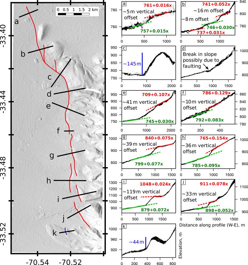
E. Hussain et al.: Seismic risk in Santiago                                                                                 1535

Ramón Fault and place it in the context of other potential        sive low noise from the point clouds by initially doing a
earthquake sources and a previous far-field subduction earth-     ground classification with only the highest points in a 3.5 m
quake (Maule 2010). As we are examining the losses due to         by 3.5 m grid and removing points that were highly isolated
a very-near-field source with exposed elements immediately        in wide and flat neighbourhoods before redoing the ground
adjacent to the potential rupture, we seek to delineate the lo-   classification with the filtered points. We then created raster-
cation, extent, and segmentation of the San Ramón Fault to        gridded digital elevation models with 10 and 2 m ground res-
improve the accuracy of the ground motion. Stereo satellite       olutions with the de-noised SPOT and Pléiades point clouds
optical imagery is often used to derive high-resolution digital   (∼ 83 and ∼ 60 million points respectively). We did this by
elevation models (DEMs) over relatively large areas, which        first triangulating the point cloud into a temporary triangular
can be useful in identifying subtle active tectonic geomorphic    irregular network (TIN) and then rasterising the TIN into a
markers of faulting as well as in examining fault segmenta-       digital elevation model.
tion (Elliott et al., 2016). In this paper we use DEMs created       The San Ramón Fault is not immediately obvious in the
from high-resolution satellite imagery from the SPOT and          Pléiades elevation map (Fig. 3) beyond the overall morphol-
Pléiades satellites (1.5 and 0.5 m resolution respectively) to    ogy of the uplifted San Ramón mountains with a relief of
better characterise the surface expression of the San Ramón       2.5 km above the Santiago basin. However the fault scarp is
Fault and to also look for other potential fault splays within    clear in the hillshaded DEM, slope and, and terrain rugged-
the city limits. Following a similar method as Chaulagain         ness index (TRI) maps (Fig. 3a, iii–v) as a north–south trend-
et al. (2016) and Villar-Vega and Silva (2017) and using          ing lineament. The terrain ruggedness index is a measure of
the Global Earthquake Model’s (GEM) OpenQuake Engine              the local variation in elevation about a central pixel (Riley
(Silva et al., 2014), we explore the contrasting losses to the    et al., 1999; Wilson et al., 2007). A TRI of 0 indicates flat
residential-building stock in the capital through scenario cal-   terrain while a value of 1 indicates extremely rugged terrain.
culations for (a) future earthquakes on the San Ramón Fault,      Such analysis can highlight the change in elevation and slope
(b) earthquakes on a hypothesised shallow splay buried be-        at a fault scarp. We use these datasets to map the surface ex-
neath the centre of the city, (c) deep intra-slab events, and     pression of the San Ramón Fault, confirming and building
(d) the 2010 Mw 8.8 Maule earthquake. Our models help us          on previous work by Armijo et al. (2010), who used a 10 m
to identify particularly vulnerable parts of the city and en-     DEM.
able us to make targeted geographical recommendations to             The identification of the active fault trace at the surface
improve the seismic resilience of these communities.              provides some evidence for the length, location, and segmen-
   We also explore losses to the non-residential-building         tation of the fault at depth, and that information is used as
stock using the Risk Management Solutions (RMS) commer-           a constraint in the subsequent risk analysis for the range of
cial risk model. The RMS model provides a different view of       earthquake sources that we seek to test. Measuring the verti-
the commercial risk, where the model is well calibrated due       cal offset across the scarp can give an idea of the past activ-
to the availability of losses from previous events and covers     ity along the fault with the caveat that due to natural erosion
the insured assets, which is often one of the main mecha-         processes, scarps tend to degrade with time. To do this we
nisms to recover from disasters.                                  plotted a series of west–east profiles across the foothills of
                                                                  the San Ramón mountains to identify and measure the scarp
                                                                  height along the fault by determining the vertical offset be-
2   Fault geomorphology from satellite imagery                    tween the best fit lines through the point cloud either side
                                                                  of the fault scarp (green and red lines in Figs. 4 and 5). The
Freely available global elevation data from the Shuttle Radar     variable topographic slope along the fault means it is difficult
Topography Mission (SRTM) (Farr et al., 2007) have a spa-         to fit lines of equal length for each profile. In most cases we
tial resolution of 30 m, which is insufficient to accurately      have tried to ensure a fit through at least 500 m, but where
map the San Ramón Fault scarp or look for other potential         possible 1 km, of points on either side of the fault scarp.
fault splays expressed in the geomorphology. To overcome             In the northern section we found scarp heights to vary be-
the low-resolution issue, we analysed SPOT-6 stereo satel-        tween ∼ 5 and ∼ 119 m along the fault trace (Fig. 4). Profile
lite imagery over a 35 km × 36 km region covering Santiago        d shows no clear evidence of a fault scarp, but since this pro-
city and the San Ramón mountains. The SPOT-6 panchro-             file is near a stream channel the scarp is moderated by fluvial
matic imagery (acquired in 2014) has a spatial resolution of      erosion. However, it contains a clear break in slope, which is
1.5 m. We also requested the acquisition of very high reso-       indicative of active faulting. Profiles c and k cross anticlines
lution (0.5 m panchromatic, acquired in 2016) Pléiades tri-       (∼ 145 and ∼ 44 m high respectively) that have likely grown
stereo imagery over a smaller region (5 km × 36 km) cover-        as a result of long-term movements in the hanging wall of the
ing just the San Ramón Fault (Fig. 2). We performed pho-          fault. The anticline shown in profile k cuts across the north-
togrammetry analysis using commercial software (ERDAS             ern section of an alluvial fan, implying its growth post-dates
IMAGINE 2015) to produce topographic point clouds from            the age of the fan deposit.
the SPOT and Pléiades stereo imagery. We removed exces-

https://doi.org/10.5194/nhess-20-1533-2020                               Nat. Hazards Earth Syst. Sci., 20, 1533–1555, 2020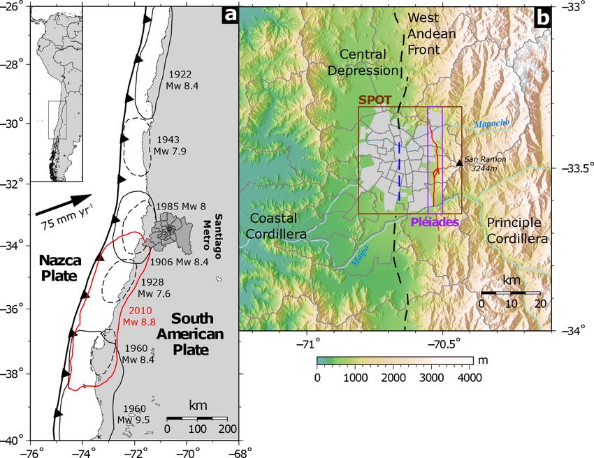
1536                                                                                     E. Hussain et al.: Seismic risk in Santiago

Figure 2. (a) Map of central Chile showing the location of great earthquakes for the past century in the subduction zone where the Nazca
plate is converging beneath the South American plate at a rate of 43 mm yr−1 (Zheng et al., 2014). The Santiago metropolitan region is
shown in the dark grey outline, subdivided by commune (names of all the communes are given in Fig. S1). (b) A 90 m SRTM shaded terrain
map of the region around Santiago city (light grey). The SPOT and Pléiades satellite data used in this study cover the region shown by the
maroon and purple polygons respectively. The San Ramón Fault is shown in red, while the dotted blue line is the location of our inferred
buried fault within the city (see text for details). The dashed black lines are the mountain front faults mapped by Armijo et al. (2010).

   In the southern section the scarp heights vary between ∼ 2          ment over numerous earthquakes. However there is signifi-
and ∼ 30 m (Fig. 5). Profiles l and m show two folds with              cant variation along the fault, with the smallest scarp of 2 m
heights of ∼ 23 and ∼ 102 m respectively. The growth of the            and the largest at 119 m. This variation is probably due to
fold in profile p (∼ 68 m high) shows evidence that it blocked         erosion along the mountain front leading to variable degra-
and diverted the Maipo river further south to its current posi-        dation of the fault scarps. The smaller scarps represent the
tion.                                                                  cumulative displacements of fewer earthquakes. While these
   Our estimate of ∼ 33 m for profile j and ∼ 39 m for pro-            observations enable us to determine the active fault segments
file g are equivalent to the 31 and 40 m estimated by Armijo           that comprise the San Ramón Fault, the variations in scarp
et al. (2010). However, our estimate of ∼ 36 m for profile h is        height mean it is difficult to trace specific historical ruptures
significantly less than their 54–60 m. The range is probably           along the fault.
due to our interpretation of the upper slope, which varies due            Our observations of the fault traces show a network of fault
to scarp degradation. This may be because of the relatively            segments that are ∼ 0.5 to ∼ 8 km long. Our assumption is
lower resolution DEM of 10 m used by Armijo et al. (2010)              that at depth these segments represent the same fault. This is
compared to our 2 m DEM.                                               motivated by field observation that large earthquake ruptures
   Our geomorphic analysis of the surface trace of the San             often consist of multiple rupture segments (e.g. Barka et al.,
Ramón Fault confirms the findings of Armijo et al. (2010) for          2002; Civico et al., 2018). It is possible that the two main
the central and northern part of the fault (red line in Fig. 3)        strands of the San Ramón Fault (Figs. 4 and 5) could rup-
and extends the trace of the fault further to the south (blue          ture independently. However, these individual fault segments
line in Fig. 3).                                                       are not long enough to produce a magnitude 7.5 earthquake
   In their trench study Vargas et al. (2014) measured fault           from a 5 m slip event, which justifies exploring earthquake
displacements of the order of ∼ 5 m. Projected to the ver-             scenarios that rupture across both strands of the fault.
tical for a 45◦ dipping fault, this gives a vertical offset of            The West Andean frontal faults drawn by Armijo et al.
about 3.5 m. Given that our average measured scarp height is           (2010) appear to terminate at the northern and southern mar-
∼ 32 m, it is likely that this represents cumulative displace-         gins of the city. Although it is possible that the San Ramón

Nat. Hazards Earth Syst. Sci., 20, 1533–1555, 2020                                      https://doi.org/10.5194/nhess-20-1533-2020
E. Hussain et al.: Seismic risk in Santiago                                                                                            1537

Figure 3. (a) (i) The Pléiades satellite optical multispectral image, (ii) the elevation map created using photogrammetry analysis of the
panchromatic optical image, (iii) the hillshaded digital elevation model (DEM), (iv) slope map, and (v) – the terrain ruggedness index (TRI).
Data gaps are on steep slopes in shadow, resulting in low contrast and inability to derive heights from stereo image matching. (b) The SPOT
satellite multispectral image (left) and the resulting hillshaded DEM (right) derived from stereo panchromatic pairs. (Pléiades © CNES,
2016; distribution by Airbus DS/Spot Image.)

Fault accommodates the full shortening across the region, it             of a fault scarp within the central regions of the city. How-
is also possible that the frontal faults extend further west be-         ever, this could be masked by urban development, or the fault
neath the city (Fig. 2b), hidden by the sediments of the cen-            could be buried, as in the case of the Pardisan thrust fault be-
tral depression. Our investigations using the SPOT satellite             neath the city of Tehran in Iran, where no primary fault is vis-
DEM and point cloud data do not show any clear evidence                  ible at the surface (Talebian et al., 2016). Similarly, the 2011

https://doi.org/10.5194/nhess-20-1533-2020                                      Nat. Hazards Earth Syst. Sci., 20, 1533–1555, 2020
1538                                                                                           E. Hussain et al.: Seismic risk in Santiago

Figure 4. The northern section of the Pléiades-derived DEM (2 m resolution) indicated in Fig. 3. The black points on the profiles are ground
pixels within a 30 m swath of the profile line from the Pléiades-imagery-derived point cloud, while the grey are from the SPOT point cloud.
The red and green lines are best fit lines through the point clouds either side of the fault scarps. The scarp height is estimated from the vertical
offset between these two lines. The blue lines are the height of anticlines measured from the downslope side.

Mw 6.3 Christchurch (New Zealand) earthquake occurred on                    same as for the San Ramón Fault. In Sect. 3 we will explore
a previously unrecognised fault buried right beneath the cen-               the losses from moderate-magnitude earthquakes (Mw 6 and
tre of the city (Elliott et al., 2012), but its impact was much             Mw 6.5) on this hypothesised buried fault within the city with
greater than the larger earthquake (Mw 7.1) that struck the                 larger magnitude events on the San Ramón Fault (Mw 7 and
year before outside of the city.                                            Mw 7.5), consistent with the palaeo-seismic trench work of
   Riesner et al. (2017) proposed a first-order model for the               Vargas et al. (2014). The magnitudes for the central Santiago
deeper structure of the San Ramón Fault and found that it                   splay scenario were determined using standard fault scaling
constitutes the frontal expression of a major west-vergent                  relationships (Wells and Coppersmith, 1994), where a rup-
fold-and-thrust belt that extends laterally for thousands of                ture with a length of ∼ 25 km, a width of ∼12 km, and a
kilometres along the western flank of the Andes (see also                   co-seismic slip of 1 m would result in an earthquake with
Armijo et al., 2015). Since it is well known that frontal faults            moment magnitude in the range of 6–6.5.
of fold-and-thrust belts tend to migrate out of the central                    In 1647 a large earthquake destroyed Santiago, which at
highlands through progressive growth of new faulting (e.g.                  the time was a 100-year-old Spanish town, and killed an es-
Davis et al., 1983; Dahlen, 1990; Reynolds et al., 2015), it is             timated one-fifth of its inhabitants (de Ballore, 1913; Udías
not unreasonable to assume that younger faults would extend                 et al., 2012). Details of this earthquake remain poorly un-
further west from the San Ramón Fault. We project the loca-                 derstood, and there is much debate on the epicentral loca-
tion of this inferred fault along strike from the West Andean               tion (e.g. Lomnitz, 1983; Comte et al., 1986; Lomnitz, 2004).
cordillera frontal fault (Fig. 2b) and assume the dip is the                Lomnitz (1970) notes that historical descriptions of the dam-

Nat. Hazards Earth Syst. Sci., 20, 1533–1555, 2020                                            https://doi.org/10.5194/nhess-20-1533-2020
E. Hussain et al.: Seismic risk in Santiago                                                                                            1539

Figure 5. The southern section of the Pléiades DEM indicated in Fig. 3. The black points on the profiles are ground pixels from the Pléiades-
imagery-derived point cloud, while the grey are from the SPOT point cloud.

age indicate an epicentre within 50 miles of Santiago at most,           3     Earthquake scenarios for the residential-building
while Poirier (2006) mentions that the earthquake did not                      stock
produce any devastating tsunamis, both pointing to a source
on a fault near the city. As there is no evidence of this earth-         The development and implementation of measures to min-
quake in the trench studies along the San Ramón Fault (Var-              imise the physical impact due to earthquakes require a com-
gas et al., 2014), it is unlikely that the earthquake originated         prehensive understanding of the potential for human and eco-
there as suggested by Rauld (2002). While it is possible that            nomic losses, which is usually achieved through earthquake
the earthquake occurred on one of the faults in the princi-              risk assessment studies (e.g. Silva et al., 2015b; Chaulagain
pal cordillera (Farías et al., 2010), our assumption was that            et al., 2016). For risk management purposes, risk is the po-
the main activity in the region is on the frontal portions of            tential economic, social, and environmental consequences of
the fold-and-thrust belt (e.g. Dahlen, 1990; Reynolds et al.,            hazardous events that may occur in a specified period of time
2015). It is also possible that the 1647 earthquake occurred             (see Grossi and Kunreuther, 2005, for details).
on the West Andean faults to the north and south of the city                We use the GEM OpenQuake Engine v3.3.2 (Silva et al.,
(Fig. 2); however, due to the lack of any evidence for either            2014; GEM, 2019) to calculate the damage and losses to
case we feel it is reasonable to explore the worst-case sce-             residential buildings from earthquake scenarios on predeter-
nario of an earthquake occurring on the extension of these               mined faults for all 52 communes that make up the Santiago
faults through the city.                                                 metropolitan region (∼ 1.1 million buildings). In the sections
   Another possible candidate for the 1647 earthquake is an              below we briefly describe the key components of the dam-
earthquake in the subducting slab beneath the city. Therefore,           age and risk calculation: exposure, hazard, and vulnerability
we also examine intra-slab faulting scenarios. This is moti-             (Fig. 6).
vated by the most damaging earthquake in terms of fatali-
ties in south central Chile in the previous century. The 1939            3.1    The residential-building exposure model
earthquake (Ms ∼ 7.8) caused ∼ 28 000 deaths (many times
more than the great 1960 subduction earthquake) and pro-                 In order to describe the residential-building stock of the San-
duced extensive damage to the city of Chillán (Saita, 1940;              tiago metropolitan region we used the exposure model es-
Frohlich, 2006), about 200 km south of Santiago. Beck et al.             tablished by Santa-María et al. (2017). The exposure model
(1998) modelled the first P-wave motions for this earthquake             was built using data from the national population and hous-
and concluded that it was a normal-faulting event within the             ing census surveys (2002 and 2012) and information from
down-going slab at a depth of 80–100 km. Since the subduct-              the 2002–2014 Formulario Único de Estadísticas de Edifi-
ing slab beneath Santiago is also about 80 km beneath the                cación (Unique Edification Statistic Form; UESF). The ex-
city (Hayes et al., 2012), we explore the losses from similar            posure model describes the number and distribution of resi-
normal-faulting events in the slab beneath Santiago.                     dential buildings at the census block resolution and contains
                                                                         information on the main material of construction, number
                                                                         of storeys (Fig. S2), age of construction, expected ductil-
                                                                         ity, the number of people living in each building, and the

https://doi.org/10.5194/nhess-20-1533-2020                                       Nat. Hazards Earth Syst. Sci., 20, 1533–1555, 2020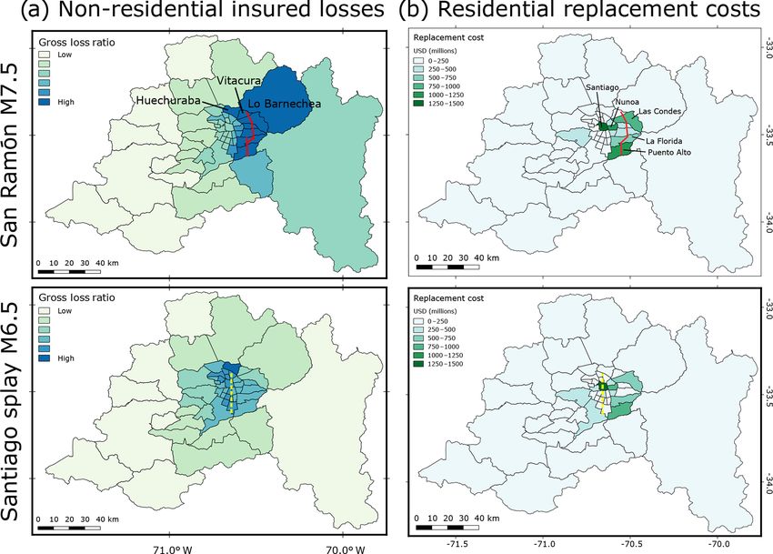
1540                                                                                  E. Hussain et al.: Seismic risk in Santiago

Figure 6. A graphical representation of the damage and loss calculation workflow using the Global Earthquake Model’s OpenQuake Engine
(Silva et al., 2014). Black boxes represent model calculators, while white boxes are data inputs/outputs.

replacement cost per unit area. The replacement cost in-             are 0.63, 0.01, 0.45, 0.20, and 0.73 for reinforced-concrete
cludes an estimate of the structural, non-structural, and con-       (RC), confined-masonry (MCF), reinforced-masonry (MR),
tent costs of each building. We assume the earthquake sce-           unreinforced-masonry (MUR), and wooden (W) buildings
narios occur at night, and therefore the residential fatality es-    respectively. It is clear that the scatter in the data for
timates represent the night-time losses. Table 1 summarises          the masonry buildings is large and reflected in the low
the most important information in the residential-building           R 2 values, particularly for MCF buildings, implying lit-
exposure model. The most commonly used building mate-                tle correlation between levels of poverty and the fraction
rial for residential buildings is masonry (79 % of all build-        of confined-masonry buildings. However, we find that the
ings), with confined masonry the dominant building typology          fraction of reinforced-concrete buildings decreases signifi-
(39 % of total buildings), followed by reinforced-masonry            cantly with the proportion of people living below the poverty
(26 %) and unreinforced-masonry structures (14 %). To im-            line. This trend is balanced by an increase in the fraction
prove computing efficiency we resample the Santa-María               of wooden, reinforced-masonry, and unreinforced-masonry
et al. (2017) exposure model from the census-block resolu-           buildings with level of poverty.
tion to a 1 km × 1 km grid (Fig. S1). Our exposure model re-
veals that Puente Alto, Maipú, and La Florida are the most           3.2   Definition of the earthquake scenarios
populated communes, together accounting for about 26 % of
all residential homes in the Santiago metropolitan region.           Unlike probabilistic seismic-hazard analysis where the risk
Puente Alto and La Florida are centred on the San Ramón              calculation is initiated with a stochastic event dataset, in
Fault.                                                               this study we calculate the damage and losses for specific
   Figure 7 shows the fraction of the total building stock           earthquake scenarios on predetermined faults. We chose a
in each commune categorised into the five building classes           scenario-based approach because it provides clear commu-
against the percentage of people living below the poverty            nication of the relative scale of potential damage and losses
line, defined as USD 400 per month for a family of four              from the recently recognised proximal San Ramón Fault
(Ministerio de Desarrollo Social, 2016). The coefficients of         versus that from the better-characterised offshore subduc-
determination (R 2 ) for the fit through each building class         tion faulting, which is important for emergency management

Nat. Hazards Earth Syst. Sci., 20, 1533–1555, 2020                                  https://doi.org/10.5194/nhess-20-1533-2020
E. Hussain et al.: Seismic risk in Santiago                                                                                       1541

Table 1. Summary of the building classes and typologies in our Santiago residential-building exposure model, based on
Yepes-Estrada et al. (2017).

              Class    Building typologies (GEM taxonomy)                                     Count    % of total   Storeys
              RC       Non-ductile reinforced-concrete walls (CR_LWAL-DNO)                    79 198        5.65       1–7
                       Ductile reinforced-concrete walls (CR_LWAL-DUH)                        72 882        5.20     1–8+
              MCF      Non-ductile confined-masonry walls (MCF_LWAL-DNO)                     395 349       28.19       1–3
                       Ductile confined masonry (MCF_LWAL-DUH)                               149 714       10.68       1–5
              MR       Ductile reinforced-masonry walls (MR_LWAL-DNO)                        259 223       18.48       1–3
                       Non-ductile reinforced masonry (MR_LWAL-DUH)                          109 430        7.80       1–5
              MUR      Non-ductile unreinforced-masonry walls (MUR_LWAL-DNO)                 161 779       11.54       1–2
                       Non-ductile unreinforced-adobe walls (MUR-ADO_LWAL-DNO)                32 160        2.29       1–2
              W        Non-ductile light-wood walls (W-WLI_LWAL-DNO)                          12 796        0.91       1–2
                       Ductile light-wood walls (W-WLI_LWAL-DUM)                             129 372        9.23       1–3
              UNK      Unknown or insufficient information available (UNK)                       319        0.02
                       Total                                                               1 402 222

                                                                         planning and for raising societal awareness of risk (Silva
                                                                         et al., 2014).
                                                                            We modelled the San Ramón Fault as a set of four rect-
                                                                         angular slip planes (total length of 35 km) to account for the
                                                                         changes in geometry along strike due to fault segmentation
                                                                         from our DEM analysis (Fig. S3). The prescribed fault planes
                                                                         dip at 45◦ to the east and extend from the surface down to
                                                                         12 km depth based on the structural cross sections drawn by
                                                                         Armijo et al. (2010) and the depth of microseismicity deter-
                                                                         mined by Pérez et al. (2014) as indicators of the down-dip
                                                                         width that is locked and accumulating strain. The location
                                                                         of the hypothesised splay fault is in line with the West An-
                                                                         dean Front and 12 km west of the San Ramón Fault, consis-
                                                                         tent with the approximate 10 km spacing inferred in the ma-
                                                                         jor thrust faults beneath the San Ramón–Farellones Plateau
                                                                         (Pérez et al., 2014). We represent the splay fault using a sin-
                                                                         gle 45◦ eastward-dipping rectangular plane extending from
                                                                         0.5 km below the surface down to 12 km depth, with a north–
                                                                         south strike running 25 km along longitude 70.65◦ W. The
                                                                         deep intra-slab fault scenario is modelled using a single
                                                                         westward-dipping rectangular plane with a length of 35 km
                                                                         in the subducting slab beneath the city. We used a 70◦ dip
Figure 7. The fraction of residential buildings by building class –      for the intra-slab fault to represent a similar earthquake to
RC is reinforced concrete, MCF is confined masonry, MR is rein-          the 1939 Chillán earthquake, for which Beck et al. (1998) es-
forced masonry, MUR is unreinforced masonry, and W is wooden             timated a 60–80◦ dipping fault plane. We used the Slab1.0
construction – against the proportion of people living below the         model (Hayes et al., 2012) to set the top depth and bottom
poverty line in the communes of the Santiago metropolitan region.
                                                                         depth of the fault plane at 85 and 98 km respectively for this
Solid lines represent best-fit trends through the data (linear for all
                                                                         locality. Earthquakes on the San Ramón and Santiago splay
cases except for reinforced concrete, which is exponential), with
coefficients of determination of 0.63, 0.01, 0.45, 0.20, and 0.73 for    faults are prescribed as having a pure thrust mechanism (rake
RC, MCF, MR, MUR, and W respectively. The poverty line is de-            +90◦ ), while the intra-slabs are normal (rake −90◦ ). The
fined as USD 400 per month for a family of four (Ministerio de           fault characteristics are summarised in Table S1.
Desarrollo Social, 2016).                                                   The hazard component of the calculation concerns de-
                                                                         termining the spatial pattern of the key shaking parameters
                                                                         from each scenario event by employing a ground motion pre-

https://doi.org/10.5194/nhess-20-1533-2020                                      Nat. Hazards Earth Syst. Sci., 20, 1533–1555, 2020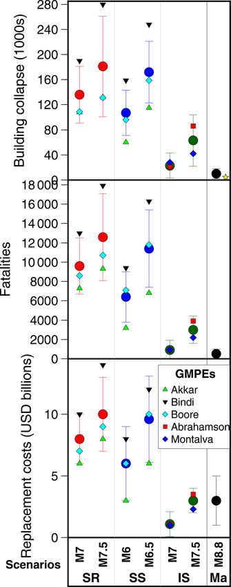
1542 E. Hussain et al.: Seismic risk in Santiago
diction equation (GMPE). The hazard parameters used here
are peak ground acceleration (PGA) and spectral accelera-
tion (SA). There are many GMPEs available in the litera-
ture (see Douglas and Edwards, 2016, for a review and http:
//www.gmpe.org.uk, last access: 1 January 2019, for an up-
dated compendium). In our analysis we use three equations
for shallow-crustal earthquakes (Akkar et al., 2014; Bindi
et al., 2014; Boore et al., 2014) and two for the intra-slab sce-
nario calculations (Abrahamson et al., 2016; Montalva et al.,
2017). These were selected for the OpenQuake Engine ac-
cording to expert opinion during the Global GMPEs project
(Stewart et al., 2012, 2015) and have been updated since.
Averaging several selected GMPEs helps to partially prop-
agate the epistemic uncertainty of the distribution of shaking
that arises from a non-perfect knowledge of ground motion.
There are several methods to calculate the distance from each
exposure point to the rupture. To remain consistent across
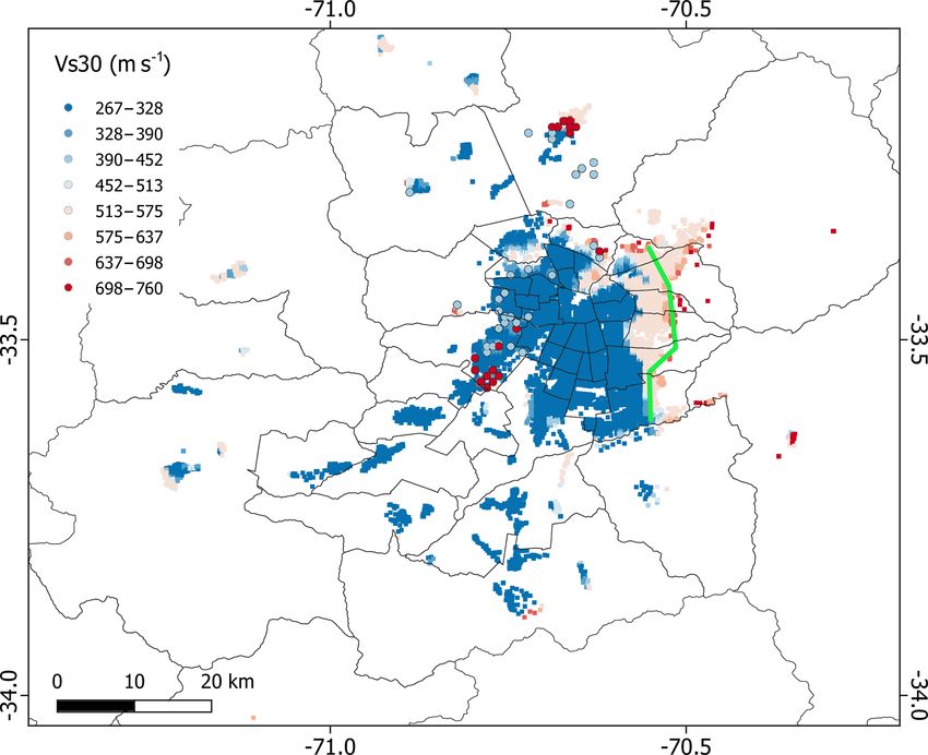
the GMPEs we implement the form of the equations that use Figure 8. A map of the Vs30: shear-wave velocity in the top 30 m
the Joyner–Boore distance, defined as the shortest horizontal of soil in metres per second at the exposure locations. The circled
distance from each exposure element to the surface projec- data are from microzonation studies (Leyton et al., 2011; Humire-
tion of the rupture area. However, we present the damage Guarachi, 2013), and the remaining are estimates derived from the
and loss results at the district level by calculating the sum of topographic slope (Allen and Wald, 2007). The green lines indicate
the losses of all points within each district. the surface trace of the San Ramón Fault used in the seismic-risk-
For each scenario we produce 1000 realisations of the scenario calculations. Red colours indicate a relatively high Vs30
ground motion in the region to account for the aleatory vari- value and are generally in regions with exposed or shallow bedrock.
ability in the ground motion and assume the entire fault rup- Relatively slow Vs30 values are associated with sedimentary basins.
tures in the earthquake. We account for the spatial correlation
of the intra-event variability during the generation of each
ground motion field according to the methods described by soil types in each zone, taking into account additional infor-
Jayaram and Baker (2009) to ensure assets located close to mation from soil penetration tests (Humire-Guarachi, 2013).
each other will have similar ground motion levels. However, given the cost and time demand of such studies,
For the 2010 Mw 8.8 Maule earthquake, we directly used microzonation maps are usually focussed on limited areas.
the USGS ShakeMap as the input ground shaking for the Therefore, for the remaining zones we supplemented the mi-
damage and risk assessment calculations (see Villar-Vega crozonation data with velocities from the USGS Global Vs30
and Silva, 2017, for details of this procedure). Map Server (Allen and Wald, 2007). This method derives
maps of seismic site conditions using topographic slope as
3.3 Site effects a proxy, assuming that stiffer materials (i.e. higher Vs30 val-
ues) are more likely to maintain a steep slope, while deep
The Santiago metropolitan region is located in a narrow basin basin sediments are deposited mainly in environments char-
between the Andes and coastal mountains filled with Qua- acterised by a lower velocity.
ternary fluvial and alluvial sediments (Armijo et al., 2010). Figure 8 shows the Vs30 values used in this study at the
Using numerical simulations of the Santiago basin taking ac- building exposure locations, with the values from the micro-
count of the superficial geology, Pilz et al. (2011) showed zonation studies indicated in circles. Note that this will prob-
that there is a strong and sometimes complex basin amplifi- ably be an underestimate of the full basin effects (Joyner,
cation effect on the peak ground velocity from hypothetical 2000). For example, not accommodating for basin resonance
earthquakes on the San Ramón Fault. While in this study we will mean that our models do not take into account the par-
are unable to account for the complexities of basin resonance ticular vulnerability of buildings of certain heights that are
and topography, we attempt to take into account the basin prone to resonance, which was an important factor for ex-
amplification effect in our ground motion calculations by us- ample in the Kathmandu rupture and basin amplification in
ing the Vs30 values, the shear-wave velocities in the top 30 m Nepal, with 4–5 s of resonance (Galetzka et al., 2015).
of soil.
In this study two datasets were used to obtain the Vs30 3.4 Building fragility and vulnerability models
information for Santiago. The first consists of local micro-
zonation studies, which contain seismic-zonation maps (Pas- The physical, or structural, vulnerability for a built system is
ten, 2007; Leyton et al., 2011) and proposed Vs30 values for defined as its susceptibility to losses when subjected to earth-
Nat. Hazards Earth Syst. Sci., 20, 1533–1555, 2020 https://doi.org/10.5194/nhess-20-1533-2020E. Hussain et al.: Seismic risk in Santiago 1543
quake shaking. In our scenario calculations we use two main single rectangular Santiago splay fault and a more complex
forms of vulnerability models: fragility functions, which are pattern from the San Ramón Fault. For the San Ramón case
used to relate earthquake shaking to certain levels of physi- most of the high ground shaking is around the communes
cal damage to a building (e.g. extensive damage, collapse), to the east of the city, while for the splay fault case there is
and vulnerability functions (structural and occupants), which a more even distribution of shaking across the central com-
relate the earthquake shaking of a structure to the economic munes.
and human losses. Our damage and loss results, averaged over the GMPEs
Villar-Vega et al. (2017) analytically derived fragility used in each scenario calculation, reveal that the collapsed-
functions for the 57 building classes in the exposure dataset building estimates for each scenario are distributed unevenly
developed for the South America Risk Assessment (SARA) across the city (Fig. 10). Figure 11 shows a summary of the
project (Yepes-Estrada et al., 2017). For our analysis we use damage and loss results for all scenarios. It is clear that the
the subset of these equations that represents the building damage and losses are greater for the larger-magnitude earth-
exposure in the Santiago metropolitan region (Table 1 and quake considered in each case as one would expect since
Fig. S1). To derive the fragility functions, Villar-Vega et al. larger earthquakes, at a given depth, produce higher-intensity
(2017) represented the structural capacity of each building ground shaking.
class by a set of single-degree-of-freedom (SDOF) oscilla- For the San Ramón scenarios the losses are mostly con-
tors. Each oscillator was subjected to a suite of ground mo- centrated in the communes around the fault. Most collapsed
tion records representative of the South American tectonic buildings are located in Puente Alto (23 100–28 800; 16 %–
environment and seismicity using GEM’s Risk Modellers’ 20 %), La Florida (12 400–15 700; 15 %–19%), and Las Con-
Toolkit (Silva et al., 2015). From each analysis, the max- des (10 500–12 800; 20 %–25 %), where the first numbers in
imum spectral displacement of each SDOF oscillator was the brackets are the building collapse counts for the two San
used to allocate it into a damage state (e.g. collapse). In this Ramón Fault scenarios and the second two numbers the per-
paper, we focus our scenario analysis on the spatial distribu- centage of collapse of the total number of exposed buildings
tion of collapsed buildings, which comprises not only phys- in the commune. We calculate fewer residential-building col-
ically collapsed buildings but also partially collapsed struc- lapses in Peñalolén (5900–7400; 14 %–17 %) and La Reina
tures (Villar-Vega et al., 2017). (5000–6200; 18 %–23 %) despite these communes also be-
The simplification of each building typology to a single- ing located on the fault. This discrepancy could be explained
degree-of-freedom oscillator means that the calculated through a combination of greater exposed population – and
fragility functions only approximate the building response thus more residential buildings (Fig. S6 shows the percentage
to ground shaking. Therefore these would not be sufficient of collapsed buildings) – and the level of poverty.
to investigate building-by-building scale losses from earth- Puente Alto has the largest population of these communes
quake shaking. However, we believe it is sufficient to ex- (622 356) and also the greatest percentage living below the
plore aggregated district level losses. And so, while the sce- poverty line (Table 2). Puente Alto and La Florida also gen-
nario calculations are done on a 1 km × 1 km gridded expo- erally contain a greater proportion of masonry constructions
sure model, the losses presented in the following sections ag- (93 % and 86 % compared to 79 % and 71 % for Peñalolén
gregate these to the district level. and La Reina respectively), which perform poorly in the
A vulnerability curve establishes the probability distribu- San Ramón earthquake scenarios. While Peñalolén has a low
tion of a loss ratio (e.g. fatalities / total number of occupants) fraction of RC residential buildings (5 %), which generally
given a shaking intensity measure level (Figs. 9 and S5). perform well in our calculation, it is compensated by a large
Vulnerability curves are generally empirically derived using proportion of wooden structures (17 %), which perform the
loss data, usually collected through insurance claims or gov- best when subject to seismic shaking.
ernmental reports. A database of fragility and vulnerability In general the greatest percentage of collapsed buildings
functions can be found in the OpenQuake platform (Yepes- (Fig. S6) occurs, as expected, in the communes directly on
Estrada et al., 2016; Martins and Silva, 2018). We used these the fault, e.g. Vitacura (3000–3600; 21 %–25 %) and Las
vulnerability functions to directly model fatalities and repair Condes (10 500–12 800; 20 %–25 %). However there are sev-
costs, where the loss ratio for the former would be the ratio eral communes with high collapse fractions that are not lo-
of fatalities to exposed population, and for the latter the ratio cated on the fault, notably Ñuñoa (8400–10 600; 20 %–25 %)
would be that of repair cost to cost of replacement for a given and Macul (4200–5300; 18 %–23 %). These both have a high
building typology. fraction of unreinforced-masonry buildings, 27 % and 13 %
respectively compared to an average of 9 % for the com-
3.5 Residential-building collapse and loss results munes on the fault (Table 2). Unreinforced-masonry build-
ings are the most likely building class to collapse in all the
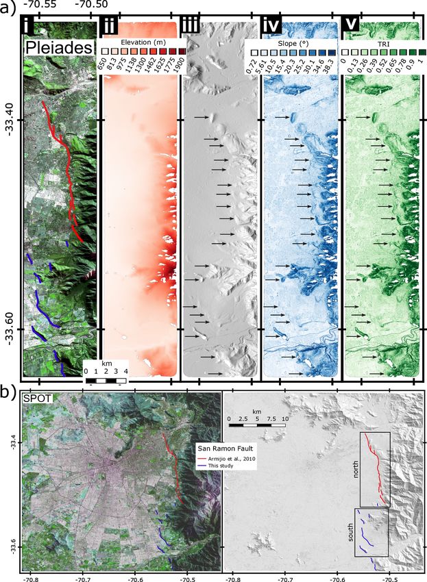
The median predicted ground motion for the larger earth- scenarios considered in this study (Table 4).
quake scenario considered for each fault is given in Fig. 9. It In terms of anticipated fatalities for the larger San Ramón
shows the relatively simple ground motion patterns from the scenario (Fig. 12), the communes of Ñuñoa and Providen-
https://doi.org/10.5194/nhess-20-1533-2020 Nat. Hazards Earth Syst. Sci., 20, 1533–1555, 20201544 E. Hussain et al.: Seismic risk in Santiago
Figure 9. The estimated median peak ground acceleration (PGA) as a fraction of gravity g for the largest earthquake scenario considered
for each fault. For the San Ramón (red line) and Santiago splay fault (green line) cases, these estimates were obtained using the Akkar et al.
(2014) ground motion prediction equation, while those for the intra-slab fault are estimates from the Abrahamson et al. (2016) equation.
The USGS peak ground accelerations for the Mw 8.8 Maule earthquake are shown at the bottom. The ground motions for the full set of
earthquake scenarios are given in Fig. S4.
Table 2. Exposed populations and buildings for the 10 most affected communes in terms of average modelled building collapse across the
six earthquake scenarios (full list in Supplement; Tables S2 and S3). The communes are ranked in order of average collapse count.
Communes Area Population Popn density Popn below Buildings in exposure model (% of total)
km2 (per km2 ) poverty line∗ (%) RC MCF MR MUR W Total
Puente Alto 88 622 356 7072 8.0 3 61 29 3 4 143 463
La Florida 71 356 925 5027 3.1 6 51 26 9 8 81 493
Santiago 22 371 250 16 875 5.9 38 19 15 27 1 57 341
Ñuñoa 17 273 354 16 080 2.4 36 32 18 13 1 42 598
Las Condes 99 296 251 2992 0.6 38 31 21 8 1 51 646
Maipú 133 608 094 4572 5.2 4 44 35 12 6 142 828
Peñalolén 54 197 909 3665 4.8 5 39 30 9 17 42 562
La Pintana 31 191 306 6171 13.9 2 39 36 10 13 40 847
Providencia 14 88 928 6352 0.7 51 25 18 6 0 22 080
Macul 13 116 694 8976 5.3 16 32 17 27 7 23 528
∗ defined as USD 400 monthly income (in 2015 US dollars) for a family of four (Ministerio de Desarrollo Social, 2016).
cia (10 km west of the San Ramón fault trace) are modelled range of 9700–12 700 (Fig. 11), resulting in a fatality rate of
as experiencing the highest fatality rates of 4–5 per 1000 0.15 %–0.19 % (Table S3). The residential losses in terms of
per 1000 people (Fig. S7). In terms of absolute numbers, replacement costs average USD 8–10 billion (5 %–7 % mean
the largest number of fatalities (Fig. 12) occurs in Ñuñoa loss ratio). The greatest replacement costs are for Santiago
and Las Condes (1120–1420 and 1080–1330 respectively). (USD 1.3 billion), but they are also high (USD 0.5+ bil-
Overall the fatalities across the region are estimated in the lion) for the communes of Puente Alto, Las Condes, and La
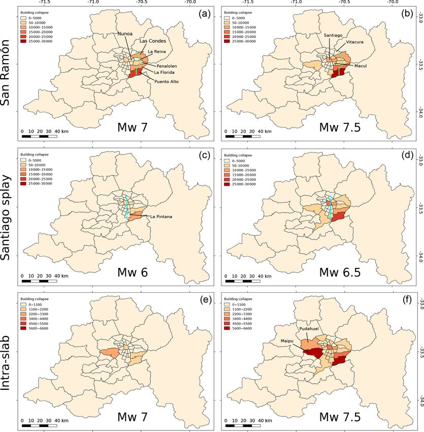
Nat. Hazards Earth Syst. Sci., 20, 1533–1555, 2020 https://doi.org/10.5194/nhess-20-1533-2020E. Hussain et al.: Seismic risk in Santiago 1545 Figure 10. The distribution of collapsed buildings for the earthquakes considered in each set of magnitude pair scenarios for the San Ramón Fault (green line; a–b), the Santiago splay fault (dashed cyan line; c–d), and a deep intra-slab fault (e–f). The collapse counts are the average for the GMPEs used in each calculation and include the total count of both complete and partial collapses. Note that the range of the colour scale changes between the upper four and lower two panels. The collapse fraction for each commune is given in the Supplement (Fig. S6). Names of all the communes are given in Fig. S1. Florida on top of the San Ramón Fault, as well as for Ñuñoa mune. Of the communes directly next to the fault splay, San- further west (Fig. S8). tiago has the largest number of residential buildings (57 341). For the earthquake scenarios on a buried fault splay be- However, the greatest impact in terms of collapse fraction neath the centre of the city, the distribution of collapsed res- is in the communes in the central districts near the fault, idential buildings is similar to the San Ramón scenario with with the highest fraction of collapse occurring in Santi- damage concentrated towards the eastern communes of the ago (10 000–15 400; 17 %–27 %), Providencia (3400–5500; city on the hanging wall of the fault. Most collapses oc- 15 %–25 %), Independencia (2500–3700; 16 %–24 %), and cur in Puente Alto (13 600–20 900; 9 %–15 %) and Santi- Ñuñoa (6600–10 300; 15 %–24 %). The estimated fatalities ago (10 000–15 400; 17 %–27 %). As in the case of the San for the buried splay scenarios are similar to or slightly above Ramón Fault the high collapse count in Puente Alto probably those for the San Ramón cases despite being a magnitude reflects the large number of residential buildings in that com- lower in scale, in the range of 6500–11 500 (0.10 %–0.17 % https://doi.org/10.5194/nhess-20-1533-2020 Nat. Hazards Earth Syst. Sci., 20, 1533–1555, 2020
1546                                                                                   E. Hussain et al.: Seismic risk in Santiago

                                                                      60 000), with most collapsed homes and fatalities (Fig. 12)
                                                                      generally located in the more populous communes. The ex-
                                                                      tent of collapse across the city is more diffusive due to the
                                                                      buried nature of the intra-slab source, with building collapse
                                                                      up to 8% in the centre (Lo Espejo, San Joaquin, and Inde-
                                                                      pendencia). The estimated total number of fatalities (Fig. 11)
                                                                      for the larger event is 3180 (0.05 %), with the largest number
                                                                      of fatalities (200–300; Table S3) each in Santiago, Ñuñoa,
                                                                      Maipú, and Puente Alto (Fig. 12). The estimated replacement
                                                                      cost is USD 3 billion (2 % loss ratio), with the greatest costs
                                                                      distributed in the same commune as fatalities (Fig. S8).
                                                                         Central government statistics estimate a total collapse
                                                                      count of 81 444 residential buildings throughout Chile in the
                                                                      2010 Mw 8.8 earthquake, with the most damage occurring
                                                                      in the Maule, Biobío, O’Higgins, and Santiago metropolitan
                                                                      regions (Elnashai et al., 2010; de la Llera et al., 2017) and
                                                                      4306 of these collapses occurring in the Santiago metropoli-
                                                                      tan region (yellow star in Fig. 11). While the collapse count
                                                                      is smaller than our modelled estimate of 9800 ± 8000, it is
                                                                      within the error margin. The discrepancy could have arisen
                                                                      due to a slightly different exposure model. The actual expo-
                                                                      sure in 2010 would have been different than our exposure
                                                                      model estimates, which use data from 2014. Moreover, there
                                                                      is often ambiguity regarding the classification of actual struc-
                                                                      tural collapse and damage beyond repair (and thus in need of
                                                                      demolition). See Villar-Vega et al. (2017) for a discussion on
                                                                      this topic.
                                                                         While we estimate building collapse fractions up to 21 %
                                                                      (Providencia) for the Mw 7 San Ramón scenario, the aver-
                                                                      age collapse ratio across all the communes is ∼ 8 %. This is
                                                                      larger than the 6.5 % estimated by Vaziri et al. (2012) for a
Figure 11. A summary of the total number of building collapses        magnitude 6.8 earthquake on the fault. However, their esti-
and fatalities as well as the total replacement costs for each sce-   mate of 14 000 fatalities is larger than the 9700 we estimate
nario calculation. The solid circles are the average across the GM-   for a Mw 7 earthquake. This difference is most likely due to
PEs considered in each scenario, which are indicated by the smaller   variations in the exposure model and calculation procedure
polygons. The spread in the estimates from the GMPEs indicates        (i.e. choice of ground motion models). But since Vaziri et al.
the epistemic uncertainty in our calculations. Error bars represent
                                                                      (2012) used an industry exposure model we are not able to
1 standard deviation determined from the 1000 Monte Carlo simu-
                                                                      determine the exact cause behind the difference in our esti-
lations. The yellow star denotes the actual number of building col-
lapses (4306) in Santiago in the 2010 Maule earthquake (Elnashai      mates.
et al., 2010).                                                           In general, across all the scenarios considered in this study,
                                                                      the largest number of collapsed buildings occurs in the highly
                                                                      populous communes (which therefore have more buildings)
                                                                      close to the fault. However, the collapse and fatality frac-
loss ratio). The most affected communes are also similar, in-         tions (the number of collapses or fatalities over the exposure;
cluding Santiago, San Miguel, Providencia, and Ñuñoa, with            Figs. S6 and S7) reveal particularly vulnerable areas. Sev-
fatality fractions of 4–5 per 1000 for the larger Mw 6.5 sce-         eral communes experience relatively large damage and loss
nario (Fig. S7). The greatest number of fatalities for both           fractions, which is an indication of the vulnerability of the
magnitudes (Fig. 12) is also in Santiago and Ñuñoa (870–              communities in these communes. Of particular importance
1600 and 710–1310 respectively; Table S3). The residential            are Ñuñoa, Providencia, and Santiago, which generally have
replacement costs are USD 6.1–9.6 billion (4 %–6 % loss ra-           high loss fractions with 3, 3, and 2 fatalities per 1000 people
tio) for the two magnitude scenarios (Table S3). The greatest         and damage fractions of 15 %, 15 %, and 15 % respectively,
losses are in Santiago, Ñuñoa, and Puente Alto (Fig. S8).             averaged over the six earthquake scenarios. In comparison
   The overall collapse count for the magnitude 7 deep intra-         the average loss fraction across all communes and all scenar-
slab scenario is small, but the magnitude 7.5 scenario re-            ios is 0.8 fatalities per 1000 people and 7 % building collapse.
sults in a substantial number of collapsed buildings (about           Therefore targeted measures to retrofit particularly vulner-

Nat. Hazards Earth Syst. Sci., 20, 1533–1555, 2020                                    https://doi.org/10.5194/nhess-20-1533-2020
E. Hussain et al.: Seismic risk in Santiago 1547
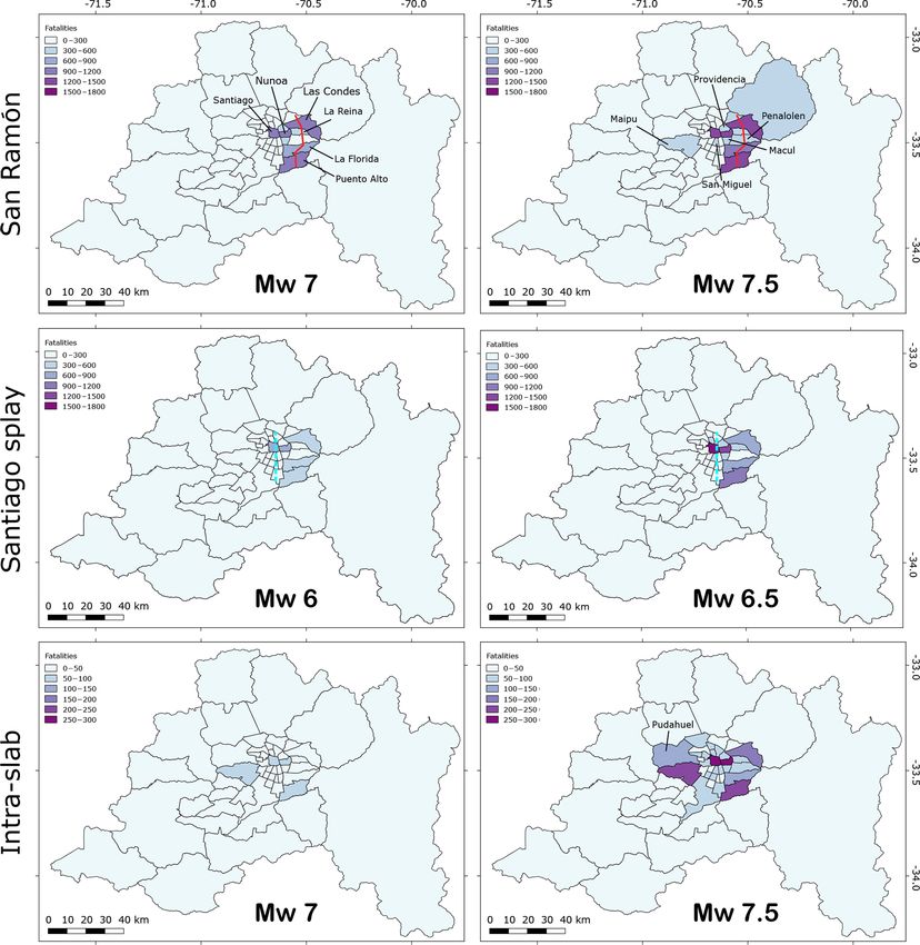
Figure 12. The estimated fatalities in each commune for the earthquakes considered in each scenario for the San Ramón Fault (red line), the
Santiago splay fault (dashed cyan line), and a deep intra-slab fault. Note that the range of the colour scale changes between the upper four
and lower two panels.
able residential buildings (unreinforced masonry) could re- as roads or bridges. The exposed values (or “total insured
duce the seismic risk faced by communities living in these value”, TIV) in this dataset include commercial buildings,
communes. contents, and business interruption and are aggregated at the
commune level.
Table 3 and Fig. 13a give a summary of the average gross
4 Non-residential insured losses loss ratios (calculated loss over the total insured value) for
the maximum-magnitude scenarios on the San Ramón and
We also used Risk Management Solutions’ (RMS) commer- Santiago splay faults. The gross losses are the full replace-
cial Chile Earthquake Model, developed in 2011, with the ment costs for the property after accounting for insurance
most recent industry exposure database (IED) to derive in- penetration and after the application of deductibles, limits,
dustry loss estimates for specific earthquake scenarios. The and co-insurance. This is often referred to as the insured
exposure model contains only non-residential-building in- loss. It is worth noting that these losses are a subset of
formation and does not include public infrastructure such
https://doi.org/10.5194/nhess-20-1533-2020 Nat. Hazards Earth Syst. Sci., 20, 1533–1555, 2020You can also read