Glacier speed-up events and subglacial hydrology on the lower Franz Josef Glacier, New Zealand
←
→
Page content transcription
If your browser does not render page correctly, please read the page content below
Glacier speed-up events and subglacial
hydrology on the lower Franz Josef Glacier,
                   New Zealand

                             by

                     Laura M. Kehrl

                           A thesis
        submitted to Victoria University of Wellington
                     in fulfilment of the
               requirements for the degree of
                      Master of Science
                         in Geology.

                  Antarctic Research Centre
              Victoria University of Wellington
                            2012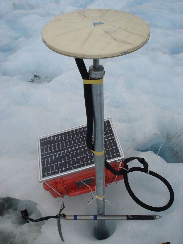
Abstract

   The contribution of glacier mass loss to future sea level rise is still poorly con-
strained (Lemke and others, 2007). One of the remaining unknowns is how water
inputs influence glacier velocity. Short-term variations in glacier velocity occur
when a water input exceeds the capacity of the subglacial drainage system, and
the subglacial water pressure increases. Several studies (Van de Wal and others,
2008; Sundal and others, 2011) have suggested that high ice-flow velocities dur-
ing these events are later offset by lower ice-flow velocities due to a more efficient
subglacial drainage system. This study combines in-situ velocity measurements
with a full Stokes glacier flowline model to understand the spatial and temporal
variations in glacier flow on the lower Franz Josef Glacier, New Zealand. The
Franz Josef Glacier experiences significant water inputs throughout the year (An-
derson and others, 2006), and as a result, the subglacial drainage system is likely
well-developed. In March 2011, measured ice-flow velocities increased by up to
75% above background values in response to rain events and by up to 32% in
response to diurnal melt cycles. These speed-up events occurred at all survey lo-
cations across the lower glacier. Through flowline modelling, it is shown that the
enhanced glacier flow can be explained by a spatially-uniform subglacial water
pressure that increased during periods of heavy rain and glacier melt. From these
results, it is suggested that temporary spikes in water inputs can cause glacier
speed-up events, even when the subglacial hydrology system is well-developed
(cf. Schoof, 2010). Future studies should focus on determining the contribution of
glacier speed-up events to overall glacier motion.
Acknowledgments
   I would like to thank a number of people who have helped me over the last
year. First, thanks to my supervisors – Huw Horgan, Andrew Mackintosh, Brian
Anderson, and Ruzica Dadic – for their support, constructive criticism, and chal-
lenging questions. I benefited from their varied expertise and skills, and each one
of them helped me with a different component of this thesis.
   I would also like to thank everyone who helped me in the field. The Depart-
ment of Conservation (DoC) permitted access to the glacier. Karen McKinnon,
Martina Barandun, Ruzica Dadic, Huw Horgan, Brian Anderson, Wolfgang Rack,
and Oliver Marsh helped haul equipment and take measurements. The Franz
Josef Glacier guides let us use their carved pathways on the glacier, which made
access to the glacier easier and safer.
   Lastly, thanks to my family and friends. My parents provided emotional sup-
port as I adjusted to a new country. My officemates – Sanne, Denise, Kathi, Karen,
Richard, and Lloyd – always managed to put a smile on my face, even when the
dark days of GPS processing nearly consumed my life. I would not be studying
glaciers today if it wasn’t for my undergraduate advisor, Bob Hawley, who first
sparked my interest in glaciology. He remains a great mentor and friend.
   Funding for the fieldwork component of this project was arranged by Andrew
Mackintosh and came from a variety of sources, including an ANZICE contract.
The Fulbright program and Antarctic Research Centre provided financial support
for my time in New Zealand. The staff at the NZ Fulbright office deserve a special
thanks for their support, encouragement, and help over the last year.
iv
Contents

1   Introduction                                                                           1
    1.1   Overview . . . . . . . . . . . . . . . . . . . . . . . . . . . . . . . . . .     1
    1.2   Glacier dynamics . . . . . . . . . . . . . . . . . . . . . . . . . . . . .       2
          1.2.1   Glacier flow . . . . . . . . . . . . . . . . . . . . . . . . . . . .     2
          1.2.2   Glacier hydrology . . . . . . . . . . . . . . . . . . . . . . . .        3
          1.2.3   Spatial variations in glacier flow . . . . . . . . . . . . . . . .       5
          1.2.4   Intra-annual variations in glacier flow . . . . . . . . . . . . .        5
    1.3   Motivation for this study . . . . . . . . . . . . . . . . . . . . . . . . .      7
          1.3.1   Franz Josef Glacier . . . . . . . . . . . . . . . . . . . . . . . .      7
          1.3.2   Research Questions . . . . . . . . . . . . . . . . . . . . . . . .       9

2   Methodology                                                                           11
    2.1   Water inputs to the glacier bed . . . . . . . . . . . . . . . . . . . . .       12
          2.1.1   Field methods . . . . . . . . . . . . . . . . . . . . . . . . . . .     12
          2.1.2   Energy balance model . . . . . . . . . . . . . . . . . . . . . .        16
          2.1.3   Discharge model . . . . . . . . . . . . . . . . . . . . . . . . .       23
    2.2   Ice-flow velocities . . . . . . . . . . . . . . . . . . . . . . . . . . . . .   24
          2.2.1   Field methods . . . . . . . . . . . . . . . . . . . . . . . . . . .     24
          2.2.2   GPS processing . . . . . . . . . . . . . . . . . . . . . . . . . .      27
          2.2.3   Uncertainty estimates at the GPS stations . . . . . . . . . . .         29
    2.3   Finite element glacier model . . . . . . . . . . . . . . . . . . . . . . .      33
          2.3.1   Governing equations . . . . . . . . . . . . . . . . . . . . . . .       33
          2.3.2   Boundary conditions . . . . . . . . . . . . . . . . . . . . . . .       35
          2.3.3   Glacier geometry and mesh . . . . . . . . . . . . . . . . . . .         36

                                             v
vi CONTENTS
2.4 Summary . . . . . . . . . . . . . . . . . . . . . . . . . . . . . . . . . . 39
3 Results 41
3.1 Water inputs to the glacier bed . . . . . . . . . . . . . . . . . . . . . 41
3.1.1 Measured rain events . . . . . . . . . . . . . . . . . . . . . . 41
3.1.2 Measured ablation rates . . . . . . . . . . . . . . . . . . . . . 42
3.1.3 Energy balance model . . . . . . . . . . . . . . . . . . . . . . 42
3.1.4 Discharge model . . . . . . . . . . . . . . . . . . . . . . . . . 44
3.2 Ice-flow velocities . . . . . . . . . . . . . . . . . . . . . . . . . . . . . 46
3.2.1 Background ice-flow velocities and strain rates . . . . . . . . 46
3.2.2 Short-term variations . . . . . . . . . . . . . . . . . . . . . . . 48
3.3 Glacier model . . . . . . . . . . . . . . . . . . . . . . . . . . . . . . . 55
3.3.1 Sensitivity to parameters As and C . . . . . . . . . . . . . . . 55
3.3.2 Sensitivity to boundary conditions in Zone 1 . . . . . . . . . 59
3.3.3 Modelled subglacial water pressures . . . . . . . . . . . . . . 60
3.4 Summary of key results . . . . . . . . . . . . . . . . . . . . . . . . . 62
4 Discussion 65
4.1 Glacier dynamics of the Franz Josef Glacier . . . . . . . . . . . . . . 65
4.1.1 Water inputs . . . . . . . . . . . . . . . . . . . . . . . . . . . . 65
4.1.2 Glacier motion . . . . . . . . . . . . . . . . . . . . . . . . . . 66
4.2 Glacier speed-up events on the Franz Josef Glacier . . . . . . . . . . 67
4.2.1 Measured glacier speed-up events . . . . . . . . . . . . . . . 67
4.2.2 Modelled subglacial water pressures . . . . . . . . . . . . . . 69
4.2.3 Inferred subglacial hydrology . . . . . . . . . . . . . . . . . . 70
4.3 Glacier speed-up events in overall glacier motion . . . . . . . . . . 72
5 Conclusions 75
5.1 Answered research questions . . . . . . . . . . . . . . . . . . . . . . 75
5.2 Future work . . . . . . . . . . . . . . . . . . . . . . . . . . . . . . . . 77List of Figures
1.1 Subglacial hydrology systems . . . . . . . . . . . . . . . . . . . . . . 3
1.2 Franz Josef Glacier . . . . . . . . . . . . . . . . . . . . . . . . . . . . 8
2.1 Study site . . . . . . . . . . . . . . . . . . . . . . . . . . . . . . . . . . 13
2.2 Photo of Franz Josef Glacier in March 2011 . . . . . . . . . . . . . . 14
2.3 Franz Josef Catchment . . . . . . . . . . . . . . . . . . . . . . . . . . 24
2.4 GPS setup . . . . . . . . . . . . . . . . . . . . . . . . . . . . . . . . . 25
2.5 Temporal overview of instrumental data collection . . . . . . . . . . 26
2.6 GPS position estimates before and after processing . . . . . . . . . . 28
2.7 Six-hour coordinate anomalies from the mean position at G07 . . . 31
2.8 Velocity uncertainty estimates from G07 and the gradient methods 31
2.9 Ice-flow velocities at G07 . . . . . . . . . . . . . . . . . . . . . . . . . 32
2.10 Glacier flowline cross section . . . . . . . . . . . . . . . . . . . . . . 34
2.11 Shape factor F along the flowline . . . . . . . . . . . . . . . . . . . . 35
2.12 Glacier flowline . . . . . . . . . . . . . . . . . . . . . . . . . . . . . . 38
2.13 Glacier surface and bed elevations along the flowline . . . . . . . . 39
3.1 Rain event totals . . . . . . . . . . . . . . . . . . . . . . . . . . . . . . 42
3.2 Ablation rates . . . . . . . . . . . . . . . . . . . . . . . . . . . . . . . 43
3.3 Spatial variability in ablation rates . . . . . . . . . . . . . . . . . . . 43
3.4 Measured vs. modelled ablation rates . . . . . . . . . . . . . . . . . 44
3.5 Ablation rates at sediment-covered stakes . . . . . . . . . . . . . . . 45
3.6 Modelled discharge vs. measured stage at Waiho Bridge . . . . . . 45
3.7 Modelled discharge vs. measured stage in June 2010 . . . . . . . . . 46
viiviii LIST OF FIGURES
3.8 Background ice-flow velocities . . . . . . . . . . . . . . . . . . . . . 47
3.9 Background strain rates . . . . . . . . . . . . . . . . . . . . . . . . . 48
3.10 Horizontal ice-flow magnitudes . . . . . . . . . . . . . . . . . . . . . 49
3.11 Changes in ice-flow velocities from the daily mean . . . . . . . . . . 52
3.12 Time of peak ice-flow velocity . . . . . . . . . . . . . . . . . . . . . . 53
3.13 Velocity direction at G02 and G07 . . . . . . . . . . . . . . . . . . . . 54
3.14 Estimated As values at the GPS stations . . . . . . . . . . . . . . . . 56
3.15 Glacier surface speed along the flowline . . . . . . . . . . . . . . . . 57
3.16 Best-fit combinations of As and C values . . . . . . . . . . . . . . . . 57
3.17 Glacier speed as a function of subglacial water pressure for differ-
ent combinations of As and C values . . . . . . . . . . . . . . . . . . 58
3.18 Modelled velocities along the flowline . . . . . . . . . . . . . . . . . 58
3.19 Sensitivity of model results to different boundary conditions in
Zone 1 . . . . . . . . . . . . . . . . . . . . . . . . . . . . . . . . . . . 59
3.20 Modelled velocities and subglacial water pressures . . . . . . . . . 61
4.1 Velocity percent increase as a function of modelled discharge . . . . 68List of Tables
2.1 Instrument locations . . . . . . . . . . . . . . . . . . . . . . . . . . . 14
2.2 Ablation stake descriptions . . . . . . . . . . . . . . . . . . . . . . . 15
2.3 Values for the constants in the energy balance model that differ
from those in Anderson and others (2010) . . . . . . . . . . . . . . . 17
3.1 Background ice-flow velocities . . . . . . . . . . . . . . . . . . . . . 47
3.2 Ice-flow velocity increases after rain events . . . . . . . . . . . . . . 50
3.3 Diurnal variations in ice-flow velocities . . . . . . . . . . . . . . . . 53
ixx LIST OF TABLES
List of Symbols
Energy balance model
  cp     specific heat of air
  cw     specific heat of water
   d     snow depth
  d∗     characteristic snow depth scale (11 mm w.e.)
dT /dh   atmospheric lapse rate
   I     incoming shortwave radiation
   g     acceleration due to gravity
  kE     exchange coefficient for latent heat
 kH      exchange coefficient for sensible heat
  k0     von Kármán’s constant
  Lf     latent heat of fusion
  Lv     latent heat of evaporation
 Lin     incoming longwave radiation
 Lout    outgoing longwave radiation
  N      day number from 1 January
   n     cloudiness
  M      melt rate
  P      precipitation rate
   p     air pressure
 QE      latent heat flux
 QH      sensible heat flux
 QG      ground heat flux
 Qm      energy available for melt
 QR      heat flux supplied by the rainfall
   q     vapour pressure of air
  qs     vapour pressure of air at the glacier surface
  Rb     Richardson stability criterion
  S      solar constant
   s     time since the last snowfall event
  T      absolute temperature
  Ta     absolute atmospheric temperature
  Ts     glacier surface temperature
  Tt     absolute terrain temperature
  t∗     timescale in albedo calculations
  ta     transmissivity of the atmosphere
  tc     transmissivity of the clouds
  U      wind speed at a height of 2 m

                                        xi
xii LIST OF TABLES
v viewfield at a given gridcell
Z solar zenith angle
z surface elevation
z0H roughness length for sensible heat
z0 roughness length for wind
α albedo
β slope angle
emissivity
ρ density
σ Stefan-Boltzmann constant
θ angle of incidence between slope normal and solar beam
ϕsun solar azimuth angle
ϕslope slope azimuth angle
Discharge model
D(t) glacier discharge
ks reservoir storage constant
R(t) rate of water flowing into the reservoir
V (t) reservoir’s volume
Flowline model
A Glen’s flow parameter
As sliding coefficient in the absence of cavitation
C coefficient that is less than the maximum local positive bed slope
F shape factor
f~ body force that describes valley wall drag
~g gravity vector
H glacier height
N effective pressure
n Glen’s flow law exponent
~ns unit vector normal to the glacier surface
P wetted perimeter
Pw subglacial water pressure
S glacier cross-sectional area
~ts unit vector tangent to the glacier surface
~u velocity vector
ub sliding speed
w glacier width
x horizontal coordinate
z vertical coordinate
α valley wall slope angle
~˙ strain rate tensor
ρ ice density
~τ deviatoric stress tensor
τe second invariant of the deviatoric stress tensor
τb basal drag
θ glacier slope angleChapter 1
Introduction
1.1 Overview
Sea level rise in the 21st century will likely displace hundreds of millions of peo-
ple from their homes, threaten sensitive marine ecosystems, and increase the in-
cidence of storm-related flooding (Lemke and others, 2007). To mitigate these
effects, it is important that we accurately predict future sea level rise (SLR). The
Intergovernmental Panel on Climate Change (IPCC) Fourth Assessment predicts
sea level rise of 0.18 to 0.60 metres (m) by 2100, but that prediction excludes the
effects of future changes in glacier dynamics on glacier mass balance, as the pro-
cesses are still too poorly understood (Lemke and others, 2007). Paleoclimate
studies (e.g., Overpeck and others, 2006) have shown multimetre per century
rises in sea level in the past, and similar rates have been suggested for the 21st
century when changes in glacier dynamics are taken into account (e.g. Hansen,
2007). In an attempt to estimate the possible contribution from glacier dynamics,
Pfeffer and others (2008) concluded that glaciers and ice caps could provide up to
an additional 0.47 m SLR by 2100. When the dynamics of the major ice sheets are
included in this approach, predicted SLR is one metre greater than when those
processes are neglected (Pfeffer and others, 2008).
An improved understanding of glacier dynamics is therefore important for
future adaptation and mitigation in response to climate change. The Franz Josef
Glacier in the Southern Alps of New Zealand provides a unique opportunity to
12 CHAPTER 1. INTRODUCTION
observe the dynamics of a fast-flowing, maritime glacier. To date, very few stud-
ies have explored the dynamics of this type of glacier; most, in fact, have focused
on continental mountain glaciers that experience a strong seasonal cycle in water
inputs to the glacier bed. At the Franz Josef Glacier, significant rain- and melt-
water reach the bed year round (Anderson and others, 2006). As variations in
water inputs are often correlated with variations in glacier flow (e.g., Iken and
Bindschadler, 1986; Jansson, 1995; Mair and others, 2001), the glacier dynamics of
the Franz Josef Glacier might differ from those of other glaciers. In this study, the
effects of varying water inputs on the daily and diurnal dynamics of the Franz
Josef Glacier are considered.
1.2 Glacier dynamics
1.2.1 Glacier flow
“Glacier dynamics” refers to the “dynamic processes” that govern glacier flow.
Glaciers flow from the accumulation area to the ablation area through two pri-
mary mechanisms: (1) internal deformation and (2) basal motion. Rates of in-
ternal deformation depend primarily on the glacier surface slope, ice thickness,
and temperature (Paterson, 1994), although longitudinal deviatoric stresses can
be important for some mountain glaciers (e.g. Hubbard, 1997). As these parame-
ters change with mass balance and climate, large variations in the rate of internal
deformation usually occur over time periods of a year or more (Vincent and oth-
ers, 2009).
Variations in glacier flow over shorter timescales typically result from changes
in the rate of basal motion. Basal motion consists of both sediment deformation
and glacier sliding. Many studies indicate a relationship between glacier sliding
and effective pressure (e.g., Lliboutry, 1958, 1968; Iken and Bindschadler, 1986;
Hooke and others, 1989). Effective pressure is the difference between ice overbur-
den pressure (proportional to ice thickness) and the subglacial water pressure. As
the subglacial water pressure increases, the effective pressure decreases and the1.2. GLACIER DYNAMICS 3 Figure 1.1: Subglacial hydrology systems after Fountain and Walder (1998): (A) a “fast,” arborescent system and (B) a “slow,” linked-cavity system. ice column tends towards flotation. High subglacial water pressures increase the rate of basal sliding through two different processes. First, high subglacial wa- ter pressures cause separation of the ice and bedrock, also known as “cavitation” (Lliboutry, 1968). This decreases friction where subglacial water pressures are high, thereby increasing the basal shear stress on the parts of the glacier that re- main in contact with the bed (Bindschadler, 1983). Second, high subglacial water pressures in cavities exert a force in the down-glacier direction, a process known as “hydraulic cavitation” or “hydraulic jacking” (Iken, 1981). As a result, fluc- tuations in the subglacial water pressure can affect ice-flow velocities on a short timescale (seasonal, daily, and diurnal). 1.2.2 Glacier hydrology The subglacial water pressure depends on both the water input to the glacier bed and the subglacial drainage system. A “fast” (channelized) drainage system can evacuate water more efficiently than a “slow” (linked-cavity) system. Con- sequently, the subglacial water pressure remains lower in a fast system than in a slow system for the same water input (Figure 1.1; Raymond and others, 1995).
4                                                CHAPTER 1. INTRODUCTION

    In a slow, linked-cavity system, water travels through a system of naturally-
occurring cavities linked by narrow orifices (Lliboutry, 1968; Kamb, 1987) and
a thin film of water at the bed (Weertman, 1964; Walder, 1982). These cavities
form in the lee of steps in the bedrock and increase in number and size as bed
roughness and sliding speed increase (Nye, 1970). This system is stable when
water inputs to the glacier bed are low (Kamb, 1987).

    In a fast, channelized system, water is routed primarily through relatively
straight, semicircular channels at the glacier bed. These channels can either be
incised into the ice (R-channels; Röthlisberger, 1972) or into the hard bed (N-
channels; Nye, 1973). For the R-channels to remain open, melting from the heat
dissipated by the flowing water must balance or exceed the inward creep of the
ice (Kamb, 1987). A fast system is therefore stable only when water inputs to the
system are sufficiently high. When water inputs drop below a certain level, the
conduits will close due to ice creep, and the drainage system will return to a slow
system (Kamb, 1987).

    The subglacial drainage system evolves in response to varying water inputs
throughout the year. In the winter, when water inputs are low, a slow system
dominates. The cavities may become constricted due to sediment build-up but
will remain open throughout the winter as long as the glacier continues to slide
along its bed (Fountain and Walder, 1998). When water inputs increase in the
spring, the slow system becomes unstable (Kamb, 1987). Initially, the drainage
system cannot handle the increased water input and the subglacial water pressure
increases, potentially leading to glacier uplift (e.g., Iken and others, 1983). This
event is known as a “spring event” (Mair and others, 2001). Over time, crevasses,
orifices, and remnants of last year’s channels start to incise. As the subglacial
water pressure is lower in a larger channel, the pressure gradient causes water
flow away from smaller channels towards the larger ones. After the spring event,
subglacial water pressures drop abruptly and remain low as long as discharge
levels remain high. The transition from a slow system to a fast system moves up
glacier to higher elevations as the melt season progresses (e.g., Nienow, 1994).
1.2. GLACIER DYNAMICS 5 1.2.3 Spatial variations in glacier flow Spatial variations in the subglacial drainage system often correlate with spatial variations in glacier flow. Areas of low subglacial water pressure act as “sticky spots” (Alley, 1993; Iken and Truffer, 1997; Fischer and others, 1999) and increase the basal drag at that location. Basal drag refers to the resistive force acting at the base of the glacier, and consequently, high basal drag leads to low rates of basal sliding. As the subglacial water pressure changes, sticky spots and their counterparts – “slippery spots” – can be destroyed or created (Fischer and others, 1999). The impact of these “spots” on nearby surface velocities extends beyond their immediate location as the ice column “smooths” basal motion as it is trans- ferred to the surface (Kamb and Echelmeyer, 1986). This is a result of longitudinal stress-coupling, or the “pulling” and “pushing” of ice nearby. The length scale over which variations in basal drag affect surface velocities is still poorly under- stood (Harbor and others, 1997). Balise and Raymond (1985) showed through an analytical model of a planar parallel-sided slab that basal velocity perturba- tions applied over a length scale of less than one ice thickness did not influence surface velocities. From field data, Mair and others (2001) concluded that sticky spots must be at least four ice thicknesses away for a high velocity event to occur at a given location on Haut Glacier d’Arolla, Switzerland. These results point to the importance of understanding the spatial distribution of subglacial water pres- sures and basal drag across the bed when interpreting intra-annual variations in surface flow velocities. 1.2.4 Intra-annual variations in glacier flow Intra-annual variations in surface flow velocities can occur on a seasonal, daily, or diurnal timescale. On a seasonal timescale, summer velocities are often greater than winter velocities (e.g., Hooke and others, 1983; Iken and others, 1983). Spring events usually mark the transition between the two. During this transition, ice- flow velocities are high as the subglacial drainage system evolves to a more ef- ficient system. At the toe of Haut Glacier d’Arolla, ice-flow velocities increased
6                                                 CHAPTER 1. INTRODUCTION

at all stakes by about 300-400% over a seven-day spring event in 1994 (Mair and
others, 2001). The increased surface motion occurred at a time of glacier uplift
and rising discharge in the proglacial stream, which was a result of high air tem-
peratures and heavy rain. Glacier uplift suggests increased separation between
the glacier and the bed, which would lead to reduced basal drag and high rates
of basal sliding. After the spring event, rises in river discharge did not correlate
with increases in the surface velocity, indicating that the subglacial drainage sys-
tem remained at a lower water pressure during these events. This suggests that
the system had evolved to an efficient, fast drainage system during the spring
event (Mair and others, 2001).

    Daily variations in ice-flow velocities, which last only a few hours or days,
can occur anytime of the year, even after a spring event. These events tend to be
more pronounced in the early part of the summer when the drainage system is
still poorly developed (e.g., Hooke and others, 1989). Ice-flow velocities at White
Glacier (Canada), Findelengletscher (Switzerland), and Midtdalsbreen (Norway)
have increased by up to 400% (Iken, 1974), 300% (Iken and Bindschadler, 1986),
and 900% (Willis, 1995) of background speeds, respectively, during these events.
In the early summer, daily events often occur during periods of significant surface
melt and in the late summer with periods of heavy rainfall (Willis, 1995).

    Similarly, diurnal cycles in ice-flow velocities tend to occur on days with pro-
nounced diurnal meltwater inputs and thereby subglacial water pressures. At
Findelengletscher, maximum daily borehole water pressures correlated with max-
imum velocities (Iken and Bindschadler, 1986). Nienow and others (2005), on the
other hand, found that peak velocities occurred during rising water pressures at
Haut Glacier d’Arolla. At Gornegletscher in Switzerland, diurnal fluctuations
in borehole water pressures occurred (Röthlisberger, 1976), but there were no
changes in ice-flow velocities (Iken, 1974). Fischer and Clarke (1997) explained
these varying results in terms of a “stick-slip relaxation process” at the glacier
bed. Subglacial water pressures rise until locally-accumulated strain in the ice
is released, perhaps as a result of a failure of a sticky spot. This process causes
an increase in the sliding rate. Once the ice has “relaxed” from the strain re-
1.3. MOTIVATION FOR THIS STUDY 7 lease, sliding velocities decrease despite higher subglacial water pressures. With this interpretation, strain release occurred at maximum water pressure at Finde- lengletscher and at a rising water pressure at Haut Glacier d’Arolla. The neces- sary water pressure for strain release did not occur at Gornegletscher, and conse- quently, the sliding velocity did not increase as a result of the diurnal variations in the subglacial water pressure. Not all glaciers experience diurnal variations in ice-flow velocities (Iken, 1974), and these variations often do not occur in the winter. As the above studies demonstrate, intra-annual variations in ice-flow veloc- ities usually occur when the water flux exceeds the capacity of the subglacial drainage system (Willis, 1995). Consequently, if a fast drainage system exists be- neath the glacier, transient speed-up events are less likely to occur. To date, most studies have focused on intra-annual variations in glacier speed on continental mountain glaciers, which have pronounced seasonal variations in water inputs and temperature. What if a glacier experiences significant melt and rain year round? Will the intra-annual variations in ice-flow velocities disappear if the subglacial drainage systems remains well-developed throughout the year? As more glaciers become subject to increased melt and rain year round as a result of climate change (e.g., Schuenemann and Cassano, 2010), it is important that we answer these questions. 1.3 Motivation for this study 1.3.1 Franz Josef Glacier The Franz Josef Glacier is a temperate, maritime glacier on the western flank of the Southern Alps, New Zealand (43◦ 29’ S, 170◦ 10’ E; Figure 1.2). The glacier ex- tends 11 km from an altitude of 2900 m to 300 m above sea level (m.a.s.l.). Mean ablation rates at the glacier tongue are 20 m a−1 water equivalent (w.e.), and pre- cipitation rates range from about 7 m w.e. a−1 at the toe to about 12 m w.e. a−1 at 600 m.a.s.l (Anderson and others, 2006). The high rates of accumulation and
8                                                    CHAPTER 1. INTRODUCTION

                                   170˚       175˚

                     −35˚   New Zealand                       −35˚

                     −40˚                                     −40˚

                             Franz Josef
                               Glacier

                     −45˚                                     −45˚

                                                     200 km
                                   170˚       175˚

Figure 1.2: Location of the Franz Josef Glacier on the West Coast of the Southern
Alps, New Zealand.

ablation lead to fast response times of 9 to 20 years (Oerlemans, 1997) and veloc-
ities on the order of 1000 m a−1 (Anderson, 2004). At the glacier terminus, melt
and heavy rainfall occur year round. Very few supraglacial streams exist on the
surface of the glacier, suggesting that water is routed to the bed at most locations.

    Very few studies have explored the dynamics and hydrology of the Franz
Josef Glacier. Anderson and others (in prep) used previously collected data to
address the intra-annual and decadal variations in ice-flow velocities. They con-
cluded that diurnal, daily, and seasonal variations likely occurred at the Franz
Josef Glacier, but it was difficult to determine the magnitude of these events as the
time interval between velocity measurements was not consistent. At nearby Fox
Glacier, Purdie and others (2008) found short-term velocity increases within 24
hours of heavy rainfall. Velocities during these events reached up to 44% greater
than background velocities, which is significantly less than the magnitude of
daily events previously discussed on Midtsalbreen, Findelengletscher, and other
continental glaciers (Purdie and others, 2008). Purdie and others (2008) did not
address diurnal variations as velocities were measured daily at Fox Glacier.
1.3. MOTIVATION FOR THIS STUDY 9
1.3.2 Research Questions
The objective of this study is to improve our understanding of the relationship
between water inputs and short-term variations in glacier speed on the Franz
Josef Glacier. In particular, I hope to answer the following questions:
1. How do ice-flow velocities vary spatially and temporally across the lower
Franz Josef Glacier? Are there daily or diurnal variations in ice-flow veloci-
ties?
2. Why do ice-flow velocities vary at this glacier? What do these results sug-
gest about the subglacial hydrology of the Franz Josef Glacier?
3. How do the dynamics of this glacier differ from those of other glaciers, and
what does this tell us about glacier dynamics in general?
The following chapters detail my approach to address these questions. In
the next chapter, the methodology is described. I combine in-situ measurements
and ice flow modelling to understand the relationship between ice-flow veloci-
ties, water inputs, and the subglacial hydrology system on the lower Franz Josef
Glacier. The results of this analysis are presented in Chapter 3 and discussed in
Chapter 4. Finally, conclusions and recommendations for future work are ad-
dressed in Chapter 5.10 CHAPTER 1. INTRODUCTION
Chapter 2

Methodology

To address the research questions outlined in Section 1.3.2, the relationship be-
tween ice-flow velocities and water inputs must be examined at the Franz Josef
Glacier. Two approaches can be taken to determine this relationship: a statis-
tical approach and a modelling approach. A statistical approach compares the
timing and magnitude of observed glacier speed-up events to water inputs. If
glacier speed increases during periods of significant water input, it can be in-
ferred that subglacial water pressures increased during that time (e.g., Iken and
Bindschadler, 1986). Water inputs can be assessed by examining river discharge
(e.g., Naruse and others, 1992) or borehole water pressures (e.g., Iken and Bind-
schadler, 1986; Nienow and others, 2005). A modelling approach, on the other
hand, moves beyond this statistical analysis in an attempt to understand the
physical processes behind the relationship.
   Both of these approaches are employed in this study. First, observational data
from March 2011 are used to understand the relationship between water inputs
and glacier velocity. Glacier velocity is determined by measuring the location of a
marker in the ice over time. Water inputs are harder to quantify, as water reaches
the bed from a variety of sources, such as runoff from the valley walls, rain, and
surface melt. As a result, this study combines point measurements and mod-
elling to determine water inputs to the glacier bed. Second, a full Stokes flowline
model is used to help interpret the observational data. The model incorporates
a Coulomb friction law (Schoof, 2005; Gagliardini and others, 2007) that relates

                                        11
12 CHAPTER 2. METHODOLOGY the subglacial water pressure, Pw , to the sliding speed, ub . The observational data can then be used to infer spatial and temporal variations in the subglacial water pressure. The following sections describe the in-situ measurements followed by the glacier flowline model. 2.1 Water inputs to the glacier bed Rain, seasonal snow melt, and glacier melt constitute the primary water inputs to the glacier bed. To quantify these inputs, in-situ measurements are combined with a distributed energy balance model. The energy balance model makes it possible to investigate water inputs across the entire glacier rather than at select measurement locations. The melt calculated from the energy balance model is used to drive a lumped-sum discharge model at the glacier tongue, following the methods of Anderson and others (2010). The resulting discharge curve provides an estimate of the total water in the glacier system over time. 2.1.1 Field methods Rain Precipitation totals can differ significantly between Franz Josef Village and the glacier terminus (Anderson and others, 2006). To quantify the precipitation at the glacier terminus, a tipping-bucket rain gauge was installed on Champness Rock, a rock outcrop about 300 m down-valley from the glacier terminus (Figure 2.1). The rain gauge had a resolution of 0.2 mm. The number of tips was totalled every minute. Ablation rates To measure ablation, a stake network of 20 2-m-long white PVC tubes was in- stalled across the lower glacier on March 4–6 (Figure 2.1). Each tube was drilled into the ice with a kovacs ice drill until it was flush with the glacier surface. These “ablation stakes” were placed on ice with different slope angles, sediment cover,
2.1. WATER INPUTS TO THE GLACIER BED 13
Franz Josef
Village
Waiho
5190000
River 10
00 20
00
0
150
0
50
0
Northing (m)
50
5185000
1000
00
00
15
15
10
00
2000
1500 0 2 km
0
10
2000
00
20
5180000
2500
Franz Josef 250
0
Glacier 00
25
1365000 1370000 1375000 1380000 1385000
Easting (m)
(a)
5185500
Ablation
S12 S11 Ablation & location
GPS station
S14 G01 G02 Ice fall
S08 S10 100 m
S15
Waterfall S09 G04
Northing (m)
S13
S17
G03 S16
First S07
5185000
G05
Ice Fall S06
S05
S04
G06
S03
S01
Second S02
Ice Fall
1371000 1371500 1372000
Easting (m)
(b)
Figure 2.1: Study site. (a) The inset map shows the location of the Franz Josef
Glacier in New Zealand. Franz Josef Village is 7 km north of the glacier. The
Waiho River originates from the glacier terminus. The black box on the lower
glacier indicates the region of focus in this study and is enlarged in (b). (b) Black
triangles, grey circles, and white circles indicate GPS stations, ablations stakes
where both ablation and GPS location were measured, and ablation stakes where
only ablation was measured. Light blue lines indicate the position of the “first”
and “second” ice falls (Figure 2.2). “Waterfall” marks the location of a large point
source of water (often called “Arthur’s Cataract”) on the lower glacier. Coordi-
nates are given in the New Zealand Transverse Mercator (NZTM) system. Ta-
ble 2.1 lists the coordinates for each instrument.14 CHAPTER 2. METHODOLOGY
Table 2.1: NZTM coordinates of GPS stations (G01–G07), GPS base station (MTP),
ablation stakes (S01–S17), and rain gauge installed on the lower Franz Josef
Glacier in March 2011. Ablation stakes S18–S20 were installed near G01.
Instrument Easting Northing
G01 1371391 5185402
G02 1371500 5185425
G03 1371545 5185191
G04 1371708 5185271
G05 1371818 5185071
G06 1371988 5184890
G07 1370929 5187748
MTP 1385224 5198418
S01 1372050 5184840
S02 1371970 5184797
S04 1371862 5184962
S06 1371971 5185040
S07 1371897 5185111
S09 1371476 5185309
S11 1371440 5185467
S12 1371340 5185470
S14 1371308 5185404
S15 1371578 5185364
S17 1371734 5185212
Rain gauge 1371038 5186475
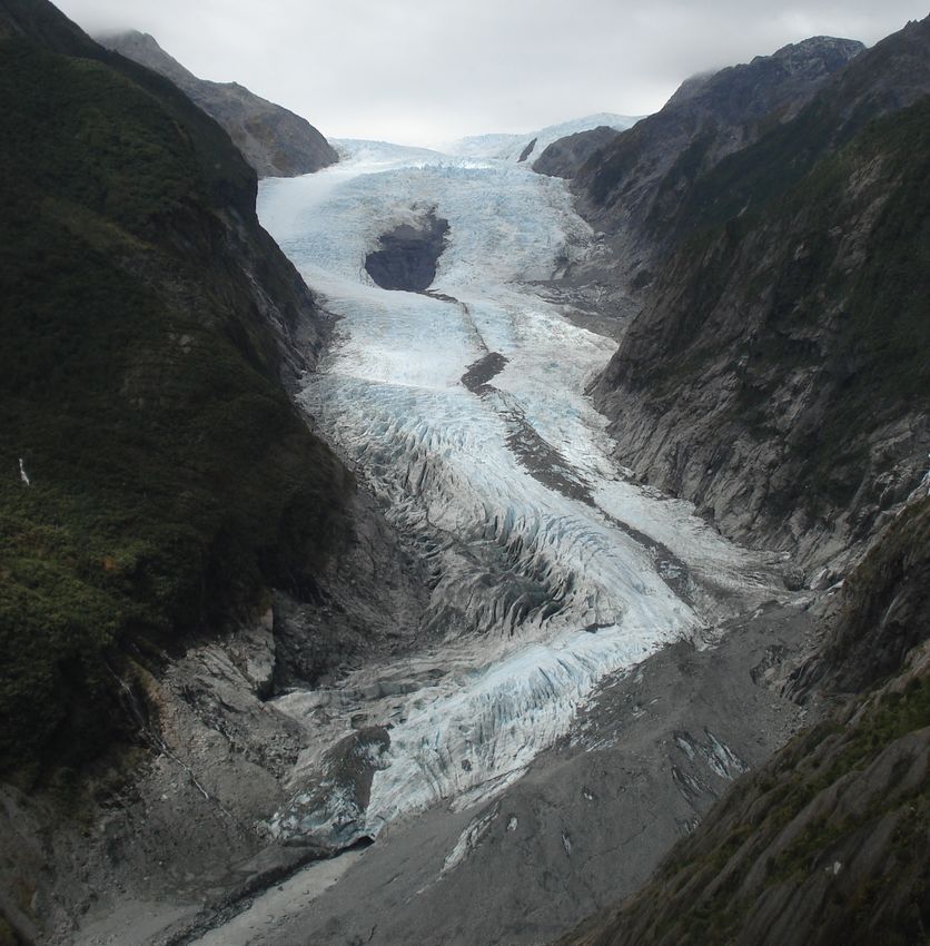
Second Ice Fall
First Ice Fall
Waterfall
Waiho River
Figure 2.2: Franz Josef Glacier in March 1
2011. Arrows point to the locations of
the waterfall, first and second ice falls, and Waiho River (Figure 2.1).2.1. WATER INPUTS TO THE GLACIER BED 15
Table 2.2: NZTM coordinates, glacier slope angle, debris cover, and ice properties
at each installed ablation stake. Four of the 20 stakes (S09, S18–S20) were located
on debris-covered ice on the medial moraine.
Stake NZTM N NZTM E Slope Debris Surface description
S01 5184653 1372045 flat none blue & bubble free ice
S02 5184616 1371969 flat none small & medium crystals
S03 5184679 1371943 low none small & medium crystals
S04 5184776 1371852 ∼20o dispersed sand hummocky surface, medium crystals
w/ veins of large crystals
S05 5184808 1371900 ∼20o dispersed sand medium crystals, meltwater pools
S06 5184857 1371966 flat none medium crystals
S07 5184925 1371893 flat dispersed pebbles small-medium crystals w/ veins of
large crystals
S08 5185160 1371394 low none small & medium crystals
S09 5185126 1371475 low medial moraine no ice exposed, large rocks and pebbles
S10 5185230 1371446 low minimal dust large crystals, ∼30% blue ice
S11 5185285 1371438 ∼10o minimal dust small crystals w/ veins of large crystals
S12 5185287 1371343 ∼20o dust on ridges hummocky surface w/ meltwater
drainage
S13 5185059 1371475 ∼30o none medium crystals
S14 5185218 1371300 ∼10o dispersed sand hummocky surface
S15 5185181 1371576 low none medium crystals, mostly blue ice w/
white striations
S16 5185020 1371664 steep none partway up crevasse, medium & small
crystals
S17 5185029 1371736 low none large crystals
S18 near G01 near G01 ∼20o medial moraine about ∼10% covered by pebbles and
rocks
S19 near G01 near G01 ∼20o medial moraine about ∼80% covered by pebbles
S20 near G01 near G01 ∼20o medial moraine no ice exposed, pebbles, rocks, & mud
and physical appearance to collect a wide range of ablation rates. Table 2.2 de-
scribes the surface appearance at each stake. Three stakes (S18–S20) were in-
stalled in varying sediment cover on the medial moraine to assess the effect of de-
bris cover on ablation rates. This is important because the energy balance model
(see Section 2.1.2) does not take debris cover into account when calculating glacier
melt. Average spacing between the remaining stakes (S1–S17) was 100–200 m.
To be consistent between ablation measurements, ablation was measured to
the nearest centimetre from the top of an ice-axe placed up-glacier of the ablation
stake. Lying an ice axe over the surface “smoothed” the centimetre-scale varia-
tions in ablation around the stake and provided a more representative ablation
rate for that stake. A constant ice density of 917 kg m−3 was assumed to convert
the measured ablation rates to water equivalent (w.e.) values. This allowed the
measured ablation rates to be compared to the modelled ablation rates calculated
by the energy balance model.16 CHAPTER 2. METHODOLOGY
2.1.2 Energy balance model
To understand ablation rates across the entire glacier, glacier melt is calculated on
an hourly timestep using a spatially-distributed energy balance model developed
by Anderson and others (2010). The energy balance at the glacier surface is given
by:
Qm = I(1 − α) + Lout + Lin + QH + QE + QR + QG , (2.1)
where Qm is the energy available for melt, I is the incoming shortwave radiation,
α is the surface albedo, Lout is the outgoing longwave radiation, Lin is the incom-
ing longwave radiation, QH is the sensible heat flux, QE is the latent heat flux, QR
is the heat flux supplied by rain, and QG is the ground heat flux. Energy fluxes
towards the glacier surface are positive and energy fluxes away from the surface
are negative. The melt rate, M , is then calculated from the available energy:
Qm
M= , (2.2)
ρ w Lf
where ρw is the density of water (1000 kg m−3 ) and Lf is the latent heat of fusion
of ice (3.34 x 10⁵ J kg−1 ).
The model requires a surface digital elevation model (DEM) and meteorologi-
cal data, including temperature, precipitation, wind speed, relative humidity, and
incoming shortwave radiation. This study uses the most-recent DEM obtained by
the Shuttle Radar Topography Mission (SRTM), which was acquired in 2000. It
has a resolution of 90 m, which is then resampled to the 100 m resolution of the
energy balance model. Hourly meteorological data are from a climate station
run by the New Zealand National Institue for Water and Atmospheric Research
(NIWA). The climate station is located in Franz Josef Village, 7 km north of the
glacier (43◦ 21’ 56” S, 170◦ 8’ 3.4” E; Figure 2.1). The temperature record from
the village is adjusted for altitude at the glacier, using a mean lapse rate, dT /dh,
of -0.005 o C m−1 , which was measured by Anderson and others (2006) between
Franz Josef Glacier and the village. Precipitation is interpolated across the glacier
using precipitation data from the village and a mean annual precipitation surface
developed by Stuart (2011). The precipitation surface is derived from a network2.1. WATER INPUTS TO THE GLACIER BED 17
Table 2.3: Values for the constants in the energy balance model that differ from
those in Anderson and others (2010).
Constant Value Units
dT /dh -0.005 oCm−1
zice 0.027 m
zsnow 0.0012 m
of climate stations across the Southern Alps and describes the mean spatial distri-
bution of precipitation from 1971–2000. The model calculates snow accumulation
from the precipitation data using a threshold of 1o C to differentiate between rain
and snow. This value has been used previously in snow modelling studies in
New Zealand (e.g., Anderson and others, 2006). The values for relative humidity
and windspeed are assumed to be the same at the village and on the glacier.
Using these inputs, the energy balance model is run from April 1, 2010 to
March 31, 2011. The following sections are modified from Anderson and others
(2010) and describe how the energy fluxes are calculated from the climate data.
A list of parameter values can be found in Table 2.3.
Shortwave radiation
Incoming solar radiation at a given location, I, depends on the solar constant,
cloudiness, atmospheric composition, and shadowing by surrounding slopes. It
includes a direct component, Idir , and a diffuse component, Idif . In complex
terrain, diffuse radiation can originate from (1) radiation reflecting off nearby
slopes, (2) backscattered radiation from the atmosphere, and (3) radiation initially
scattered through the atmosphere, known as “sky radiation” (e.g., Dozier, 1980;
Hock, 2005). In this study, diffuse radiation originating from nearby slopes is ne-
glected. The resulting diffuse component can then be described as (Oerlemans,
1992):
π
Idif = [0.8 − 0.65(1 − n)]S sin ( − Z), (2.3)
2
where n is the cloudiness, S is the solar constant, and Z is the solar zenith angle.
The solar constant, which describes the total amount of energy falling at normal18 CHAPTER 2. METHODOLOGY
incidence outside the earth’s atmosphere, changes throughout the year as a result
of changes in the Earth-Sun distance:
2πN
S = 1365[1 + 0.034 cos ( )], (2.4)
365
where N is the day number from 1 January.
The direct component of the incoming shortwave radiation, Idir , is only calcu-
lated for unshaded gridcells (Corripio, 2003; Oerlemans, 1992):
Idir = [0.2 + 0.65(1 − n)]S cos θ, (2.5)
where θ is the incidence angle between the slope normal and the solar beam given
by Garnier (1968):
cos θ = cos β cos Z + sin β sin Z cos (ϕsun − ϕslope ), (2.6)
where β is the slope angle, and ϕsun and ϕslope are the solar and slope azimuth
angles, respectively.
The distribution between direct and diffuse shortwave radiation depends on
the cloudiness, n, as scattering increases with water vapour in the atmosphere. It
is given by (Oerlemans, 1992):
I = ta tc (Idif + Idir ), (2.7)
where ta and tc are the transmissivity of the atmosphere and of the clouds, re-
spectively. Following Oerlemans (1992), these values are approximated as:
π
2
− ϕsun
ta = (0.79 + 0.000024z)[1 − 0.08( π )] (2.8)
2
and
tc = 1 − (0.41 − 0.000065z)n − 0.37n2 , (2.9)
where z is the surface elevation. To calculate cloudiness, n, cloudiness is increased2.1. WATER INPUTS TO THE GLACIER BED 19
from zero until the calculated and measured incoming solar radiation at Franz
Josef Village are equal (Arnold and others, 1996).
Albedo
The magnitude of absorbed incoming shortwave radiation depends largely on
the surface albedo (Equation 2.1). The surface albedo at a given location on the
glacier, α, depends on the snow albedo, ice albedo, and snow depth:
d
α = αsnow + (αice + αsnow )e− d∗ , (2.10)
where αsnow is the snow albedo, αice is the ice albedo (0.34), d is the snow depth
in mm water equivalent (w.e.) and d∗ is the characteristic snow depth scale (11
mm w.e.). The values for constants were determined for Morteratschgletscher,
Switzerland (Oerlemans and Knap, 1998) and match well with experimental re-
sults at nearby Brewster Glacier (Anderson and others, 2010).
The snow albedo varies both in space and time due to differences in sediment
concentration, crystal structure, and solar elevation (e.g., Wiscombe and Warren,
1980; Warren, 1982). Although local variations in sediment cover are important
for understanding differences in ablation over short distances, debris cover is
neglected in this study. Snow crystal structure changes with time, and as a re-
sult many albedo models parameterise snow albedo as a function of time. Snow
albedo is calculated following the methods of Oerlemans and Knap (1998), in
which snow albedo is dependent on the time since the last snowfall event:
s
αsnow = αf irn + (αf rsnow + αf irn )e t∗ , (2.11)
where αf irn is the firn albedo (0.53), αf rsnow is the fresh snow albedo (0.9), s is
the time since the last snowfall event (days), and t∗ is a timescale (21.9 days) that
determines how quickly the snow albedo decreases after a snowfall event.20 CHAPTER 2. METHODOLOGY
Longwave radiation
The Stefan-Boltzmann law describes the longwave radiation emitted from a black-
body:
L = σT 4 , (2.12)
where L is the longwave radiation, is the emissivity, σ is the Stefan-Boltzmann
constant (5.6704 x 10⁻⁸ W m−2 K−4 ) , and T is the absolute temperature of the ob-
ject. Outgoing longwave radiation from the glacier, Lout , is constant (317 W m−2 ),
assuming the glacier surface is at the melting point and the emissivity of snow
is 1.
Incoming longwave radiation, Lin , is emitted by the atmosphere and the sur-
rounding terrain. The partitioning between these sources is dependent on the sky
viewfield, v, defined as the fraction of unobstructed sky at each gridcell (Corripio,
2003):
Lin = ef f σTa4 v + t σTt4 (1 − v), (2.13)
where the first term describes the longwave radiation from the atmosphere and
the second term describes the contribution from the terrain. Here ef f is the effec-
tive atmospheric emissivity, Ta is the air temperature, and t is the terrain emis-
sivity (0.4; Plummer and Phillips, 2003). The terrain temperature, Tt , is set to
atmospheric temperature for terrain that is not covered by snow or ice and to 273
K for terrain that is ice- or snow-covered. The effective atmospheric emissivity,
ef f , is given by Konzelmann and others (1994):
ef f = c (1 − np ) + oc np , (2.14)
where the clear-sky emissivity, c , is
ea 1
c = 0.23 + 0.484( )8 . (2.15)
Ta
The term n is the cloudiness, oc is the emissivity of an overcast sky (0.924), and ea
is the vapour pressure.. The exponent, p = 1, is used following experimental re-2.1. WATER INPUTS TO THE GLACIER BED 21
sults at nearby Brewster Glacier (Anderson and others, 2010). Brewster Glacier is
also located on the West Coast of New Zealand and therefore experiences similar
atmospheric conditions to Franz Josef Glacier.
Turbulent heat fluxes
The turbulent heat fluxes, QH (sensible heat) and QE (latent heat), are caused by
temperature and moisture gradients between the glacier surface and overlying
air and by the wind (Brutsaert, 1982). In this study, the parameterisation of Oke
(1987) is used:
QH = ρcp kH U (Ta − Ts ), (2.16)
q − qs
QE = 0.622ρkE U Lv , (2.17)
p
where ρ is the air density, cp is the specific heat capacity of air, kH and kE are
the exchange coefficients, U is the wind speed at 2 m above the surface, Ts is the
surface temperature, Lv is the latent heat of vaporisation (2.3 x 10⁶ J Kg−1 ), q is
the vapour pressure of the air, qs is the vapour pressure of air at the glacier sur-
face, and p is the air pressure. The glacier surface temperature, Ts , is assumed
to be 0 o C. The exchange coefficients for sensible and latent heat, kH and kE , de-
termine the effectiveness of the heat transfer and relate the turbulent flux to the
temperature and wind speed gradients. They depend on the roughness length
for momentum, z0 , roughness length for temperature, z0H , roughness length for
water vapour, zOE , and the atmospheric stability. The atmospheric stability is
calculated after Oke (1987):
k02 2
kH = z (1 − 5.2Rb ) , (2.18)
log zz0 log z0H
k02 2
kE = z (1 − 5.2Rb ) ,
log zz0 log z0E
where k0 is von Kármàn’s constant (0.4), z is the measurement height (2 m above
the surface), and Rb is the Richardson stability criterion. The stability correction
term in Equation 2.18 ((1 − 5.2Rb )2 ) is only used for stable stratification (Rb < 0).
When Rb > 0 or U < 1, the stability correction term is removed. Unreasonably22 CHAPTER 2. METHODOLOGY
high bulk Richardson numbers can occur when wind speeds are low (U < 1),
which in Oke’s model, lead to the disappearance of turbulence and to a decou-
pling of the snow surface from the atmosphere above (Oke, 1987). The Richard-
son stability number, Rb , is given by:
g (Ta − Ts )(z − z0 )
Rb = , (2.19)
Ta U2
where g is the acceleration due to gravity (9.81 m s−2 ). The model assumes a con-
stant roughness length for momentum, temperature, and water vapour, which
varies over snow and ice (Anderson and others, 2010). The roughness length for
snow, zsnow , is set to 0.0012 after Anderson and others (2010) on Brewster Glacier.
The roughness length for ice, zice , is tuned to 0.027 m to minimise the difference
between modelled and measured ablation rates by Brian Anderson from 2010-
2011.
Rainfall heat flux
Assuming the rain and air temperatures are the same, the rainfall heat flux, QR ,
is given by:
QR = cW P Ta , (2.20)
where cW is the specific heat of water (4.186 J g−1 o C) and P is the rate of rainfall
(m h−1 ).
Ground heat flux
The ground heat flux is the heat flux from the glacier surface to depth. It is diffi-
cult to calculate as it depends on the available subsurface energy and the temper-
ature profile within the glacier, which are usually not known. In this model, it is
assumed that the glacier remains at 0 o C, which is a a reasonable approximation
for a temperate mountain glacier (Oerlemans, 1992). The ground heat flux, QG , is
then set to 1 W m−2 (Neale and Fitzharris, 1997; Anderson and others, 2010).2.1. WATER INPUTS TO THE GLACIER BED 23
2.1.3 Discharge model
Discharge is calculated from the modelled glacier melt using a linear-reservoir
model (Baker and others, 1982; Hock and Noetzli, 1997). This model is not spatially-
distributed. The glacier is split into three reservoirs: snow, firn, and ice. The snow
reservoir encompasses all water inputs above 2000 m, the firn reservoir includes
water inputs between 1800 m and 2000 m, and the ice reservoir includes water
inputs below 1800 m as well as all inputs off the glacier (Anderson and others
(2010)). The water that enters each reservoir is a combination of the modelled
ice melt, seasonal snow melt, and precipitation within the catchment (Figure 2.3).
The rate of change of each reservoir’s volume is given by:
dV
= R(t) − D(t), (2.21)
dt
where R(t) is the rate of water flowing into the reservoir. The discharge at the
glacier terminus, D(t), is proportional to the reservoir’s volume, V (t), at time t:
D(t) = ks V (t), (2.22)
where ks is the storage constant. Each reservoir has a different storage constant,
with ksnow = 350, kf irn = 30, and kice = 16, following values tuned at Storglaciären
(Hock and Noetzli, 1997) and at nearby Brewster Glacier (Anderson and others,
2010). As discharge was not measured during the study period, it is not possible
to tune these values to the Franz Josef Glacier. Consequently, the storage con-
stants used in this study may not be correct for the Franz Josef Glacier, although
Hock and Noetzli (1997) suggested that the discharge model may be relatively in-
sensitive to the chosen storage constants (see Section 4.1.1). Combining the above
equations and solving for discharge leads to:
1 1
D(t2 ) = D(t1 )e− ks + R(t2 ) − R(t2 )e− ks . (2.23)
The resulting discharge curve is qualitatively compared to stage data recorded
by a sonic ranger at the Waiho Bridge, which is 6 km downstream from the Franz24 CHAPTER 2. METHODOLOGY
2 km
1300
Waiho
5190000
Stage 900
500
Northing (m)
50
0
5185000
900
0
900
1300
130
90
21
0
0
1700 1700
0
17
00
21
00
5180000
1365000 1370000 1375000 1380000
Easting (m)
Figure 2.3: Franz Josef Catchment used in the discharge modelling. River stage
was recorded at the Waiho Bridge, 6 km downstream from the glacier terminus.
Josef Glacier (Figure 2.3). Stage is recorded at this location to monitor flooding
events, and Stefan Beaumont from the West Coast Regional Council provided the
data for this study. Discharge values cannot be calculated from the stage data as
stream velocity and bed geometry are not known. Furthermore, the Waiho River
is a braided river, and the location and bed geometry of the major channels can
change quickly (Davies, 1997). Modelled discharge values are used only qualita-
tively in this study.
2.2 Ice-flow velocities
To determine the spatial and temporal variations in glacier flow, six GPS stations
were installed on the lower glacier. Repeat point measurements were also taken
at 11 ablation stakes to improve the spatial resolution of the velocity measure-
ments.
2.2.1 Field methods
GPS stations
Six GPS stations (1 Trimble 5700 and 5 Trimble Net RS units; G01–G06) were
installed on the lower glacier on March 3–4 and removed from the glacier on2.2. ICE-FLOW VELOCITIES 25 Figure 2.4: Each GPS station included a zephyr antenna, solar panel, 2-m-long metal pole, and GPS receiver (in the orange box). The ice axe is for scale. March 19, 2011 (Figure 2.1 and Table 2.1). To capture the small-scale spatial varia- tions in glacier flow, GPS stations were positioned 1–2 ice thicknesses apart (Truf- fer, 2004; Gudmundsson and Raymond, 2008). Four of the stations (G01–G04) formed a grid below the first ice fall with an average spacing of 150 m (Figures 2.1 and 2.2). The remaining two stations (G05–G06) were installed roughly along centerline above the first ice fall, with a spacing of 200 m. Each GPS station included a 33 AH battery, 20 W solar panel, solar controller, GPS receiver, and zephyr antenna installed on a 2-m-long metal pole that ex- tended about 0.5–1.0 m above the glacier surface (Figure 2.4). Due to the high ablation rates on the Franz Josef Glacier, the metal pole had to be re-drilled at all stations on March 10. The stations recorded position every 15 seconds. A GPS base station (G07) was also installed on Teichelmanns Rock, a veg- etated rock outcrop about 1.5 km down-valley from the glacier terminus. The addition of a base station permitted a double-differencing (DD) algorithm to be utilised during GPS processing (see Section 2.2.2). Unfortunately, it was later dis- covered that the satellite coverage at Teichelmanns Rock was poor (typically 4–6 satellites) and that processing the kinematic stations against a GeoNet station on the 11-km-distant Mt. Price (MTP) provided better results. The GPS station on Mt. Price recorded position every 30 seconds, so the GPS units on the glacier had to be down-sampled to that rate. On March 9, the GPS stations started to turn off due to low battery voltage, as
26                                               CHAPTER 2. METHODOLOGY

        Rain gauge
            Ablation
                 G01
                 G02
                 G03
                 G04
                 G05
                 G06
                 G07
               MTP

                   2     4    6     8    10    12     14   16    18    20
                                         March 2011

Figure 2.5: Temporal overview of instrument data collection. The GPS stations
(G01–G07) shut down at various times due to low battery voltage. The dashed
appearance of G01–G04 is a result of the satellite coverage dropping to 3 satel-
lites from 03:00–05:00 each day; consequently, position estimates cannot be deter-
mined during that time. Ablation rates were recorded every 1–2 days.

the solar panels were not providing adequate power to recharge the batteries. On
March 15–16, batteries were replaced at five of the stations (G01–G05) and an ad-
ditional solar panel was installed at the remaining station (G06). After this point,
all stations, except G06, recorded data for the rest of the study period. Figure 2.5
shows when the various instruments, including the GPS stations, collected usable
data.

Repeat stake location measurements

To supplement the GPS stations, stake locations were recorded with a Trimble
GNSS handheld GPS unit at 11 of the 20 ablation stakes every 2–4 days (Fig-
ure 2.1). The stake locations were chosen to increase the spatial coverage and
resolution of the background velocity and strain rate datasets. The sampling rate
was 1 Hz. Stake occupations during the point measurement readings ranged
from 10–20 minutes depending on the reported satellite coverage from the Trim-
ble GNSS unit.
2.2. ICE-FLOW VELOCITIES 27 2.2.2 GPS processing GPS stations The kinematic GPS data are processed with TRACK (version 1.24; Chen, 1998), the kinematic module of the GAMIT/GLOBK software package (King and Bock, 2010). TRACK uses a DD approach to determine the integer phase ambiguity at each epoch. The phase ambiguity, which is a multiple of the carrier phase, must be resolved to a new integer value after every cycle slip. TRACK calculates initial ambiguity estimates using the Melbourne-Wubena Wide Lane (MW-WL; Melbourne, 1985; Wubbena, 1985), which determines the difference between the L1 and L2 phases. These estimates do not have to be integer values. Integer am- biguities are then resolved through a “relative rank” algorithm, which compares the “best“ and “next best” choices for the integer phase ambiguity based on their “chi-squared” values. The chi-squared value depends on (1) the match of the ionosphere-linear combination (LC) to the estimated value, (2) the match of the MW-WL to the average MW-WL value, and (3) the closeness of the ionospheric delay to zero. If the difference in chi-squared values between the two choices is large, then the ambiguity is resolved to the best choice integer. TRACK then applies a Kalman smoothing filter to the position estimates. There are several ways to improve the results from TRACK, including esti- mating a priori coordinates for the base and kinematic stations before processing. Base station coordinates are calculated using a precise point positioning (PPP) algorithm implemented by NASA’s online Automatic Precise Positioning Service (APPS), which uses the GIPSY/OASIS software (version 5; Zumberge and others, 1997). Rough, initial coordinates for the kinematic receivers are estimated with a module in GLOBK that calculates point position using GPS code range data. These rough estimates are iterated to more precise coordinates with subsequent runs of TRACK. The kinematic stations are then processed with the estimated locations, LC combinations, and precise ephemerides provided by the International GPS Ser- vice. GPS motion is loosely constrained in the east, north, and vertical directions
You can also read