Pervasive diffusion of climate signals recorded in ice-vein ionic impurities - The Cryosphere
←
→
Page content transcription
If your browser does not render page correctly, please read the page content below
The Cryosphere, 15, 1787–1810, 2021
https://doi.org/10.5194/tc-15-1787-2021
© Author(s) 2021. This work is distributed under
the Creative Commons Attribution 4.0 License.

Pervasive diffusion of climate signals recorded in
ice-vein ionic impurities
Felix S. L. Ng
Department of Geography, University of Sheffield, Sheffield, UK

Correspondence: Felix Ng (f.ng@sheffield.ac.uk)

Received: 5 August 2020 – Discussion started: 7 September 2020
Revised: 5 March 2021 – Accepted: 5 March 2021 – Published: 13 April 2021

Abstract. A theory of vein impurity transport conceived two       1   Introduction
decades ago predicts that signals in the bulk concentration of
soluble ions in ice migrate under a temperature gradient. If
valid, it would mean that some palaeoclimatic signals deep in     Chemical impurity concentrations in ice cores yield diverse
ice cores (signals from vein impurities as opposed to matrix      palaeoclimatic information (e.g. Legrand and Mayewski,
or grain-boundary impurities) suffer displacements that up-       1997; Wolff et al., 2006). As with other ice-core proxies,
set their dating and alignment with other proxies. We revisit     such as stable water isotopes, it is generally hoped that post-
the vein physical interactions to find that a strong diffusion    depositional modification of signals in such records, which
acts on such signals. It arises because the Gibbs–Thomson         may hamper their interpretation, is minimal. For signals of
effect, which the original theory neglected, perturbs the im-     abrupt or discrete (e.g. volcanic) events, of interest is whether
purity concentration of the vein water wherever the bulk im-      their position and shape record their timing and magnitude
purity concentration carries a signal. Thus, any migrating        faithfully. If, for instance, signals diffuse in the ice, neigh-
vein signals will not survive into deep ice where their dis-      bouring peaks may merge as they descend towards the ice-
placement matters, and the palaeoclimatic concern posed by        sheet base. Conceivably, a range of physico-chemical pro-
the original theory no longer stands. Simulations with sig-       cesses may distort signals, limiting the resolution and accu-
nal peaks introduced in shallow ice at the GRIP and EPICA         racy of the retrievable information.
Dome C ice-core sites, ignoring spatial fluctuations of the          In a landmark paper, Rempel et al. (2001) proposed a the-
ice grain size, confirm that rapid damping and broadening         ory to show that signals in the bulk concentration of dissolved
eradicates the peaks by two-thirds way down the ice column.       ionic impurities – major ions such as SO2−          −
                                                                                                               4 , Cl , and Na
                                                                                                                                 +

Artificially reducing the solute diffusivity in water (to mimic   – in the water veins at polycrystalline grain junctions (Nye,
partially connected veins) by 103 times or more is necessary      1989; Mader, 1992a, b) migrate relative to the ice when a
for signals to penetrate into the lowest several hundred me-      temperature gradient is present. Driven by what they term
tres with minimal amplitude loss. Simulations incorporating       “anomalous diffusion”, migration occurs in the direction of
grain-size fluctuations on the decimetre scale show that these    rising temperature and displaces signals with minimal distor-
can cause the formation of new, non-migrating solute peaks.       tion, so their apparent age deviates from their true age. Rem-
The deep solute peaks observed in ice cores can only be ex-       pel et al. (2001) calculated cumulative signal displacements
plained by widespread vein disconnection or a dominance           of ∼ 0.1–1 m in the lowest kilometre of the GRIP ice core.
of matrix or grain-boundary impurities at depth (including        Their mechanism could decouple the ion records from other
their recent transfer to veins) or signal formation induced by    ice-core proxies and cause significant age errors in palaeo-
grain-size fluctuations; in all cases, the deep peaks would not   climatic histories, especially in deep ice where temperature
have displaced far. Disentangling the different signal contri-    increases markedly towards the bed. This has prompted eval-
butions – from veins, the ice matrix, grain boundaries, and       uation for signs of anomalous diffusion in some ice-core
grain-size fluctuations – will aid robust reconstruction from     records (e.g. Tison et al., 2015) and simulation of the mi-
ion records.                                                      gration of specific species (e.g. methane sulfonic acid in firn;
                                                                  Osman et al., 2017). Note that it is non-trivial to infer the

Published by Copernicus Publications on behalf of the European Geosciences Union.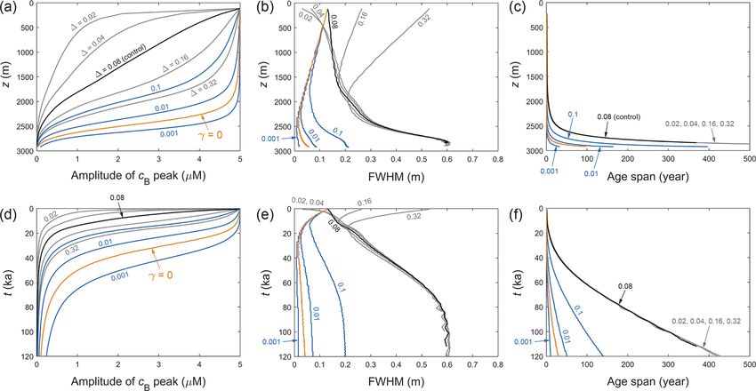
1788                                   F. S. L. Ng: Pervasive diffusion of climate signals recorded in ice-vein ionic impurities

Figure 1. High-resolution records of dissolved ionic impurities in ice cores from Antarctica and Greenland, illustrating the occurrence and
expressions of high peaks and signals at decimetre or shorter scales in deep ice. Vertical axes plot the total impurity concentration in bulk
ice (this differs from our model variable cB , which refers only to impurities in the water-vein network); 1 ng g−1 is equivalent to 1 ppb or
1 µg L−1 . (a) The sulfate record from the EPICA Dome C core, Antarctica, measured by fast ion chromatography (Traversi et al., 2009); the
arrow locates panel (b). (b) Zoomed portion of (a) showing two sulfate peaks. (c) A piece of the sodium record from the NEEM ice core,
Greenland (Schüpbach et al., 2018), from continuous-flow analysis (CFA) measurements, showing large fluctuations on a stretch with high
base level in 2187–2190 m as well as isolated peaks. (d) A piece of the sulfate record from the NGRIP ice core, Greenland (Svensson et al.,
2013), measured by CFA, showing successive sub-decimetre-scale spikes. Gaps in (c) and (d) reflect missing data.

absence or amount of migration by comparing the records                  peaks in ice cores from Antarctica and Greenland. Much of
of signal peaks from different cores, due to uncertainty in              our analytical and numerical work (Sects. 2 and 3) is spent on
depth–age scales, a lack of rigorous independent control of              understanding the origin of the strong diffusion and showing
where individual peaks should lie, and spatial inhomogeneity             its operation. We also correct the signal migration speed and
in the atmospheric dispersal and deposition of impurities by             show that grain-size fluctuations can cause new impurity sig-
environmental events. Some studies contend that signal mi-               nals to form. At the end (Sect. 4) we discuss what the revised
gration may be limited – and thus the ion records dependable,            theory means for the provenance of the deep ionic peaks in
because solute transport is hindered by disconnections in the            ice-core records.
vein network (Barnes et al., 2003; Barnes and Wolff, 2004)                  Following Rempel’s framework, we model processes be-
or because most ionic impurities are located at grain bound-             low the firn–ice transition and one ion species only (SO2− 4 is
aries (Barnes and Wolff, 2004) or in salt micro-inclusions               used in our calculations). We let cB denote its bulk concen-
within ice crystals (Ohno et al., 2005), instead of in veins.            tration, using the unit mol L−1 or M to refer to the amount
How extensively ice-core chemical records have been altered              of impurity in a unit volume of ice. Note that cB accounts
by anomalous diffusion is unresolved, despite the relevance              only for impurities dissolved in the water veins and excludes
of this question to the synchronisation of ice-core age scales           impurities at grain boundaries and in the ice matrix (inside
(e.g. Severi et al., 2007; Fujita et al., 2015) and dating of            grains), which are not modelled in this paper. Chemical al-
palaeoclimatic events.                                                   teration of signals via cation–anion associations (e.g. Iizuka
   Here we re-examine “Rempel’s theory” of vein impurity                 et al., 2004; Traversi et al., 2009), reaction of vein impuri-
transport (i.e. Rempel et al., 2001), discovering missing el-            ties with dust (Barnes and Wolff, 2004), the segregation of
ements in it that change the predicted signal evolution. We              impurities to locations outside the veins and thermodynamic
find that the relevant processes cause diffusion of signals at           coupling between multiple ion species (Rempel et al., 2002;
rates that threaten their survival in ice cores, whether or not          Rempel and Wettlaufer, 2003) are ignored.
a temperature gradient drives their migration. Hence the the-               Before plunging into mathematics, we first outline our
ory’s implications are radically revised. Our purpose is not             main finding; see Fig. 2a–d, where z denotes depth. In Rem-
to develop the theory of migrating signals to show how it can            pel’s theory, a centimetre- or decimetre-scale peak in the
match observed ion records or be used in reconstructions, but            bulk solute concentration cB , representing a climate signal,
to highlight the contrary: it struggles to explain the presence          is mirrored by variations in the porosity φ (Fig. 2c, d), which
of distinct ionic peaks in deep ice. Figure 1 exemplifies such           represents the volume fraction of veins in the ice. With cB

The Cryosphere, 15, 1787–1810, 2021                                                           https://doi.org/10.5194/tc-15-1787-2021
F. S. L. Ng: Pervasive diffusion of climate signals recorded in ice-vein ionic impurities                                               1789

Figure 2. Interactions that cause the signal migration mechanism of Rempel et al. (2001) and our signal diffusion mechanism, and variables
studied in this paper. (a) Conceptualisation of the vertical profiles of vein impurity concentration c and ice temperature T in an ice core; z
is depth below the surface. The gradients shown here typically occur over the kilometre length scale and are most pronounced towards the
base of an ice sheet; see Fig. 4 for real examples of T (z). Panels (b), (c), and (d) expand on the variations around a cB signal, which occur
at a much shorter scale of decimetres or centimetres. (b) Vein impurity concentration c. (c) Porosity φ. (d) Bulk impurity concentration cB .
(e) Vein cross-sectional geometry, showing the definition of the radius of curvature rv . (f) Equilibrium vein conditions as the solution of
model equations. An increase in cB lifts the solution A to A’, causing a perturbation on c (see panel b) that drives cB diffusion. Neglect of
the Gibbs–Thomson effect in the theory of Rempel et al. (2001) causes the bold curve in (f) to collapse onto the vertical dashed line; then no
perturbation arises to diffuse the signal.

encapsulating vein impurities, the relation cB = cφ holds1 ,             terfacial effect is small is given in their companion papers
where c, the solute concentration of the vein water, is deter-           (Rempel et al., 2002; Rempel and Wettlaufer, 2003). Then
mined by temperature T through the liquidus. A background                c depends on T only, not on cB . However, we find that
temperature gradient in the ice sets up a gentle gradient in             when this seemingly reasonable approximation is not made,
c, driving downward solute diffusion through the vein net-               the cB signal causes a perturbation on c(z) that drives non-
work (Fig. 2a). Interestingly, the porosity modulates the so-            negligible solute diffusion away from the peak (Fig. 2b), ow-
lute diffusion flux so that on the trailing (upper) edge of the          ing to the short length scale of the signal. Consequently, the
signal peak dφ/dz > 0 increases this flux with distance to               cB peak experiences pronounced broadening and amplitude
draw down cB , whereas on the leading (lower) edge of the                reduction. In an ice core, these conspire with vertical com-
peak, dφ/dz < 0 reduces the flux with distance to bump up                pression to regulate the evolving peak shape.
cB . Thus the peak signal in cB translates (the same transla-               Besides Rempel et al. (2001), Barnes et al. (2003) have
tion applies to trough signals). This mechanism is “anoma-               modelled vein-mediated evolution of dissolved ion signals
lous” because solute diffusion causes the signal to move with-           below the firn–ice transition. Their main interest was to ex-
out signal diffusion, i.e. without changing its shape. In their          plain the signal diffusion found in the top 350 m of the
calculations, Rempel et al. (2001) neglected the small effect            EPICA Dome C ice core (EPICA community members,
of the vein-face curvature on the melting point (the Gibbs–              2004), which they inferred from observed trends of peak
Thomson effect), and a detailed justification of why this in-            broadening and damping in the sulfate and chloride records
                                                                         with age. To explain the signal diffusivities estimated for
    1 Rempel et al. (2001) formulated their model with φ as a mass       these ions – respectively 4.7 × 10⁻⁸ and 2 × 10⁻⁷ m2 yr−1 ,
fraction (instead of volume fraction) and used a correspondingly         they conceived two models of vein solute transport driven by
different unit for cB , but the interactions are the same.

https://doi.org/10.5194/tc-15-1787-2021                                                          The Cryosphere, 15, 1787–1810, 2021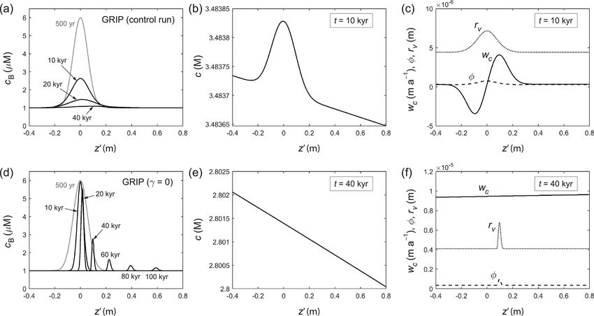
1790                                   F. S. L. Ng: Pervasive diffusion of climate signals recorded in ice-vein ionic impurities

grain growth, motivated by the fact that the mean grain size in     This equation features in earlier studies of the subject (Nye,
their stretch of the core increases with depth. One model in-       1991; Mader, 1992b; Rempel et al., 2001, 2002; Rempel and
vokes local gradients in c induced by porosity change during        Wettlaufer, 2003; Barnes et al., 2003; Dani et al., 2012). The
spatially non-uniform normal grain growth; this mechanism           three terms on its right-hand side describe the temperature
requires the presence of grain-size variations at the length        depressions due to (i) solute, (ii) interfacial curvature (the
scale of the cB signals. The other, an analogue model, uses a       Gibbs–Thomson effect), and (iii) pressure, respectively; ρi is
cell-based simulation to demonstrate how the disconnection          ice density, L is latent heat, and γ is the interfacial energy.
of veins by grain growth (modelled as random removal of             Table 1 lists the constants used in this paper, and Table 2 lists
cells and relocation of their impurity to neighbouring cells)       our model variables. For the first term in Eq. (5), a linear
causes diffusion even when the vein network is only partially       approximation θc = 0c is valid at temperatures not far be-
connected. Both models predict no diffusion of cB unless            low the melting point, e.g. 0 = 4.53 K M−1 for SO2−     4 . The
there is net grain growth.                                          third term is typically small and may be absorbed into T0 by
   We do not incorporate the Barnes et al. (2003) mechanisms        accounting for glaciostatic overburden. Accordingly, the ver-
into our model here, as the “Gibbs–Thomson diffusion” is            sion of Eq. (5) that we use for the present analysis is
much faster than their diffusion (by an order of magnitude
at least), and adding the latter strengthens our conclusions.                           γ T0
                                                                    T0 − T = 0c +             ,                                  (6)
Our mechanism is independent of grain growth and occurs                                ρi Lrv
in the absence of grain-size variations. We do, however, ac-
count for the continual motion of veins during grain bound-         but our simulations in Sect. 3 for specific ice-core sites will
ary migration, which causes a slow “residual diffusion” on          use Eq. (5), together with detailed nonlinear empirical for-
cB . This mechanism does not require a temperature gradient         mulas for θc and θp (Appendix A).
or grain-size variations to operate and is unaffected by vein          Given dg , T , and cB , Eqs. (4) and (6) can be solved for rv
disconnection.                                                      and c (e.g. Barnes et al., 2003). Figure 2f illustrates the so-
                                                                    lution as the intersection point of two curves. In their theory,
                                                                    Rempel et al. (2001) employed the liquidus relation without
2     The model                                                     including the Gibbs–Thomson term, and Rempel et al. (2002)
                                                                    and Rempel and Wettlaufer (2003) argued that under glacio-
2.1      Key relationships                                          logical conditions, a large rv makes the Gibbs–Thomson term
                                                                    negligible so that 0c ≈ T0 −T ; then c(z) is dictated by the ice
We treat polycrystalline ice in a continuum description with        temperature profile (Fig. 2a). This approximation amounts to
variables as functions of position x = (x, y, z) and time t.        taking the intersection point in Fig. 2f to lie on the dashed
Ice with the mean grain size dg (grain diameter) has the vein       line. However, as shown by Fig. 2f, the exact solution for
length density                                                      c does depend on cB – albeit weakly – for fixed T and dg .
       3                                                            This dependence lies at the heart of our “Gibbs–Thomson
l≈        ;                                                 (1)
      dg2                                                           diffusion”. Specifically, when γ T0 /ρi Lrv  0c, a first-order
                                                                    approximate solution of Eqs. (4) and (6) is
we adopt equality in this expression herein. If the vein faces
have the radius of curvature rv (Fig. 2e; Nye, 1989), then the                            γ T0
ice porosity φ is                                                   0c ≈ (T0 − T ) −            ,                                (7)
                                                                                         ρi Lrv
φ = αrv2 l,                                                 (2)                  r
                                                                                       cB dg2 0
where α = 0.0725 is a geometrical factor (Nye, 1991; Mader,         where rv ≈       3α(T0 −T ) ,   or
1992a, b). Recalling the relation between the bulk solute con-           "                                   #
                                                                                            s
centration and the solute concentration of the vein water,             1               γ T0 3α(T0 − T ) −1/2
                                                                    c≈     (T0 − T ) −                 cB      .                 (8)
cB = φc,                                                    (3)        0               ρi L    dg2 0

and using Eqs. (1) and (2), leads to                                This differs from Rempel’s approximation by the γ (Gibbs–
dg2 cB                                                              Thomson) term, which causes ∂c/∂cB > 0 and a perturbation
       = crv2 .                                           (4)       to appear on c(z) where cB (z) exhibits a signal (Fig. 2b, d).
 3α
                                                                    The rate of signal diffusion stemming from this minute per-
   For ice at a temperature T below the reference temperature       turbation will be quantified later. The result in Eq. (8) also
T0 , thermodynamic equilibrium between ice and vein water           shows that fluctuations in dg and T could perturb c(z) to
means that the liquidus relation is satisfied:                      drive solute transport and influence cB . We will explore the
                   γ T0                                             potential effect of grain-size fluctuations (Sect. 3.4), but not
T0 − T = θc +            + θp .                             (5)     temperature fluctuations, as these decay quickly in ice.
                  ρi Lrv

The Cryosphere, 15, 1787–1810, 2021                                                       https://doi.org/10.5194/tc-15-1787-2021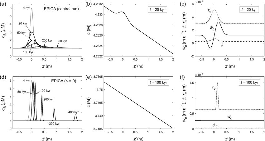
F. S. L. Ng: Pervasive diffusion of climate signals recorded in ice-vein ionic impurities                                                              1791

Table 1. Constants used in this study.

                    Symbol        Value                            Parameter
                    α             0.0725                           Geometric constant
                    c1            2.5                              Geometric constant
                    D             5 × 10⁻¹⁰ m2 s−1                 Solute diffusivity in vein watera
                    γ             0.034 J m−2                      Interfacial energy (Gibbs–Thomson coefficient)
                    0             4.53 K M−1                       Slope of water–SO2−                      ◦
                                                                                       4 liquidus curve, ≈ 0 C (Dani et al., 2012)
                    g             9.81 m s−2                       Gravitational acceleration
                    K0            1.68 × 107 mm2 yr−1              Grain growth rate constantb
                    L             333.5 × 10³ J kg−1               Latent heat of melting
                    ρi            917 kg m−3                       Ice density
                    ρw            1000 kg m−3                      Water density
                    Q             42.4 kJ mol−1                    Grain growth activation energy
                    R             8.314 J K−1 mol−1                Gas constant
                    T0            273.15 K (0 ◦ C)                 Reference temperature (melting point at 1 bar)
                  a One-third of the molecular diffusivity in water; see Rempel et al. (2001). b Value derived from Table 3.1 of Cuffey and Paterson
                  (2010), after multiplying by 6/π to correct for sectioning and stereological effects (Ng and Jacka, 2014).

Table 2. Variables in our mathematical model and their units.

                             Symbol                 Physical meaning, unit
                             c                      Impurity concentration of the vein water, M
                             cB                     Bulk impurity concentration (vein-water component only), M
                             dg                     Mean grain size (diameter), m
                             g(t)                   Depth–age scale (i.e. depth of ice having the age t), m
                             H                      Ice thickness, m
                             K                      Grain growth rate, m2 yr−1
                             l                      Vein length density, m−2
                             m                      Melt rate (mass rate per unit volume of ice), kg m−3 yr−1
                             q                      Vectorial percolative water flux in ice (scalar, q), m yr−1
                             rv                     Radius of curvature of vein faces, m
                             t                      Time, yr (when referring to age in an ice core, a is used)
                             T                      Temperature, K or ◦ C
                             u                      Ice velocity vector, m yr−1
                             uc                     Anomalous velocity vector (scalar, wc ), m yr−1
                             w̃                     Ice velocity in a reference frame following ice material, m yr−1
                             x (= (x, y, z))        Cartesian coordinate in 3D, m (see next item for orientation)
                             z                      Depth below ice-sheet surface, m
                             z0                     Vertical displacement in a reference frame following ice material, m
                             1                      Width parameter of Gaussian function, m
                             θc (/θp )              Melting-point depression due to impurity (/ pressure), K
                             κ                      Residual diffusivity due to random vein motion, m2 yr−1
                             φ                      Porosity, dimensionless

   If, instead of Eq. (6), the full liquidus relation Eq. (5)                           2.2     Porosity, water, and solute conservation
is analysed, with θc = f (c) being a mildly nonlinear func-
tion, then the above findings are qualitatively unchanged, and
                                                                                        The rest of the model is now formulated, for ice deform-
Eq. (8) would read c ≈ f −1 ([ ]) with [ ] as given in Eq. (8)
                                                                                        ing with velocity u = (u, v, w). As the porosity is very
except that f −1 (T0 − T ) replaces (T0 − T )/ 0 in the square
                                                                                        small, φ ∼ 10−6  1, the incompressibility condition ∇ ·u =
root.
                                                                                        0 holds. The total transport flux of porosity is uφ − κ∇φ.
                                                                                        The first term here describes advection by ice. The second
                                                                                        (Fickian) term describes a net transport of porosity due to
                                                                                        the random, unceasing vein motion that accompanies grain

https://doi.org/10.5194/tc-15-1787-2021                                                                               The Cryosphere, 15, 1787–1810, 2021
1792                                 F. S. L. Ng: Pervasive diffusion of climate signals recorded in ice-vein ionic impurities

boundary migration. We detail its physical derivation in Ap-       As is well rehearsed in their theory, the advection term here
pendix B. The diffusivity κ is given by                            predicts migration of chemical signals at the velocity uc rel-
                                                                   ative to the ice, with uc controlled by the temperature profile
     K(T )                                                         via the liquidus and Eq. (14). Our analyses are to reveal de-
κ=         ,                                                (9)
      3c1                                                          partures from these predictions.
where K = K0 exp(−Q/RT ) is the temperature-dependent
                                                                   2.3   One-dimensional model
grain growth rate, R is the gas constant, Q is activation en-
ergy, and c1 ≈ 2 to 3 (we use 2.5 in our simulations).             For an ice core beneath a flow divide or summit, where the ice
  Accordingly, porosity conservation is described by               motion is downward (u = (0, 0, w)) and horizontal variations
∂φ                   m                                             in φ and cB are negligible, Eqs. (10) and (15) become (on
   + ∇ · (uφ − κ∇φ) = ,                                    (10)    using ∇ · u = 0 again)
∂t                   ρi

where the melt rate m accounts for phase change occurring at       ∂φ       ∂φ     m    ∂       ∂φ
                                                                       +w       = +           κ      ,                      (17)
the interfacial boundaries of the veins; m is the rate of mass      ∂t      ∂z     ρi ∂z        ∂z
melted per unit volume of ice. This result can also be derived
from ice mass conservation.
                                                                   ∂cB          ∂cB ∂       ∂      ∂cB       ∂wc
   If q is the water flux percolating through the vein network,        +(w+wc )    + (qc) =      κ       −cB     , (18)
then water mass conservation requires                               ∂t           ∂z ∂z      ∂z      ∂z        ∂z

      ∂φ
                                                                  where wc = −(D/c)∂c/∂z is the anomalous velocity down-
ρw        + ∇.(q + uφ − κ∇φ) = m,                          (11)    ward. Equation (18) tracks the evolution of the bulk impurity
      ∂t
                                                                   profile cB (z, t) and its signals, but the water flux q needs to
and we deduce from this together with Eq. (10) that                be found via
                   m                                               ∂q           m
∇ · q = −(1 − r)      ,                                    (12)       = −(1 − r) ,                                            (19)
                   ρi                                              ∂z           ρi
where r = ρi /ρw ≈ 0.92 is the ratio of ice density to water       with m calculated from Eq. (17). This problem is supple-
density.                                                           mented by Eqs. (4) and (5) (or 6), which give the instanta-
   The local solute transport flux is ucB +qc−Dφ∇c−κ∇cB .          neous distributions of c and φ from the depth profiles of cB ,
This describes the summed effects of advection by ice and          T , and dg . There are five equations (Eqs. 4, 5, 17–19) for the
water flow, molecular diffusion in vein water, and random          five unknowns cB , c, φ, q, and m.
vein motion (the same as that driving porosity diffusion; Ap-
pendix B); D is the diffusion coefficient for the ionic impu-      2.4   Correction to the signal migration velocity
rity in water, and the diffusivity κ was defined in Eq. (9). The
corresponding solute conservation equation is                      Here we explain the first departure from Rempel’s original
                                                                   predictions: the migration speed will be faster than wc , be-
∂cB                                                                cause of water percolation induced by the migration. To see
    + ∇ · (ucB + qc) = ∇ · (φD∇c + κ∇cB ).                 (13)
 ∂t                                                                this, we need to put all advective parts of Eq. (18) (notably
                                                                   ∂(qc)/∂z) in terms of cB . Let c(z) be time-invariant as in
Following Rempel’s theory, we define the “anomalous veloc-
                                                                   Rempel’s theory, and ignore the κ-term (vein motion), to
ity”
                                                                   write Eq. (18) as
          ∇c
uc = −D                                                    (14)        ∂φ ∂q                  ∂cB          ∂wc      ∂c
          c                                                        c      +       + (w + wc )      = −cB        −q .
                                                                       ∂t    ∂z                ∂z           ∂z      ∂z
and use cB = φc to rewrite the D contribution in Eq. (13) to
derive                                                             Substituting for ∂q/∂z from Eq. (19), using Eq. (17) for m,
                                                                   converts this to
∂cB
    + ∇ · [(u + uc )cB + qc] = ∇ · (κ∇cB ).                (15)
                                                                       ∂cB      ∂cB

                                                                                            ∂cB
 ∂t                                                                r        +w         + wc     =
                                                                        ∂t       ∂z          ∂z
If both water flux q and the κ-term (“residual diffusion”
due to vein motion) are ignored, this simplifies, after using            ∂wc       ∂c             ∂c
                                                                   − cB       − q − (1 − r)wφ .                           (20)
the incompressibility condition ∇ · u = 0, to the Rempel et                ∂z      ∂z             ∂z
al. (2001) equation:                                               The z derivatives on the left-hand side describe signal advec-
∂cB                                                                tion by ice flow and anomalous diffusion, respectively. Fol-
    + (u + uc ) · ∇cB = −(∇ · uc )cB .                     (16)    lowing the scaling argument in the Supplement of Rempel et
 ∂t

The Cryosphere, 15, 1787–1810, 2021                                                   https://doi.org/10.5194/tc-15-1787-2021
F. S. L. Ng: Pervasive diffusion of climate signals recorded in ice-vein ionic impurities 1793
al. (2001), all terms on the right, based on the background of ∇T . Both the diffusion and advection terms in Eq. (23)
gradient in c (Fig. 2a), are negligible on the length scale of are controlled by D because they originate from the molec-
climatic signals (.10−1 m). In Eq. (20), the prefactor r of ular diffusion of solute in vein water. Setting γ → 0 (which
the time derivative means that the migration speed is wc /r, forces 0c ≡ T0 − T ) recovers Rempel’s theory.
which exceeds wc by ≈ 9 %. How fast do signals diffuse? One way to gauge their rate
What causes this correction? As introduced in Sect. 1, of broadening and damping versus migration is by taking
a migrating cB peak is mirrored by a moving variation in the magnitude ratio of the two terms in the square bracket
porosity. This evolution implies freezing and melting on the in Eq. (22):
peak’s trailing edge and leading edge (Fig. 2c), causing water s
to be expelled from and absorbed into these regions, respec- γ T0 3α(T0 − T ) −3/2 |∇cB |
χ= cB . (24)
tively, owing to the density change during phase change (see 2ρi L dg2 0 |∇T |
Eq. 19). Hence a water flow localised about the peak trans-
ports solute in the same direction to speed up its migration. The dimensionless number χ, which also sizes diffusion
Although modest in size, the correction applies at all depths against advection in Eq. (23), resembles the inverse of the
and also in the three-dimensional model. Péclet number in fluid mechanics. But the context here is
unique as our model concerns the transport of bulk concen-
2.5 Diffusion of impurity signals tration signals, and the underlying physics involve the geom-
etry of the vein network and two-phase (solute–ice) thermo-
The second (more crucial) departure from Rempel’s predic- dynamic equilibrium.
tions is that signals in cB will diffuse, as we emphasised at As an example, taking T0 − T ∼ 25 K, |∇T | ∼
the outset. In Rempel’s theory, cB signals suffer no distortion 20 K km−1 = 0.02 K m−1 , dg ∼ 5 mm, cB ∼ 1 µM, and
as they migrate under anomalous diffusion except for a slight |∇cB | ∼ 1 µM/10 cm = 10−5 M m−1 (a decimetre-scale
amplitude change due to the right-hand side of Eq. (16). But signal), which roughly approximate conditions in the lower
as anticipated in Sect. 2.1, they will perturb c(z) to drive so- third of the GRIP and EPICA ice cores, gives χ ∼ 1.7.
lute diffusion (Fig. 2). The consequence can be studied via The effective diffusivity in the right-hand term of Eq. (23)
a stripped-down version of Eq. (15) (or 16) where ice flow, is then 2.1 × 10⁻⁶ m2 yr−1 , which is much higher than
water flow, and vein motion (residual diffusion) are ignored: the diffusivities reported by Barnes et al. (2003) (Sect. 1).
Although these ballpark estimates depend on the chosen
∂cB
+ ∇ · (uc cB ) = 0 . (21) values (including the signal magnitude) and will change if
∂t we consider elsewhere in the ice column, they show that
For the anomalous velocity, substituting for c from Eq. (8) diffusion can pervasively modify signals, whose short length
into Eq. (14) yields, after some algebra, scales play a key role in amplifying the perturbations on c to
cause diffusion at a rate rivalling migration. We confirm this
∇c by numerical simulation next.
uc = − D
c
" s #
D γ T0 3α(T0 − T ) −3/2 3 Ice-core numerical experiments
≈ ∇T − cB ∇cB .
(T0 − T ) 2ρi L dg2 0
Using the model above, which revises and extends Rempel’s
(22)
theory, we proceed to simulate the distortion of impurity sig-
Note that this result assumes that dg varies slowly. If grain nals in ice cores in both Greenlandic and Antarctic settings,
size fluctuates strongly over short distances (e.g. decimetres), by doping shallow ice with chemical peaks and seeing how
the evaluation of ∇c would introduce another term involving they evolve. Most experiments explore predictions with a
∇dg (Sect. 3.4). With the present result in Eq. (22), Eq. (21) fully connected vein network, but we include some that sim-
becomes ulate partial disconnections (“blocked veins”) by decreasing
the molecular diffusivity D.
∂cB D∇T
+∇ · cB = 3.1 Material reference frame and set-up
∂t T0 − T
−1/2
s !
γ T0 3α cB ∇cB A general simulation of Eqs. (4), (5), and (17)–(19) would
D ∇· √ . (23)
2ρi L dg2 0 T0 − T couple them to time-varying velocity, temperature, and grain-
size distributions in the ice column. But while the corre-
This partial differential equation implies not only signal mi- sponding ice flow and thermal calculations are well estab-
gration driven by ∇T , but also signal diffusion, due to the lished (e.g. Cuffey and Paterson, 2010), reliable grain-size
right-hand (Gibbs–Thomson) term, which encapsulates the modelling remains out of reach, especially for deep ice,
c perturbation. The diffusion is nonlinear and independent where the way in which the mean grain size dg is governed
https://doi.org/10.5194/tc-15-1787-2021 The Cryosphere, 15, 1787–1810, 20211794 F. S. L. Ng: Pervasive diffusion of climate signals recorded in ice-vein ionic impurities
Figure 3. (a) Submergence velocity w(z) in an ice core and the corresponding (b, c) z–t and z0 –t plots of material trajectories. The bold
line in (b) is the depth–age relation. In (c), z0 is a depth coordinate that measures distance from ice located on the depth–age relation in (b).
The z0 -reference frame thus moves with that ice as it descends towards the bed, and material trajectories that do not start at the surface at
t = 0 converge towards z0 = 0 due to vertical compression. An impurity signal centred initially at z0 = 0 can migrate by anomalous diffusion
into z0 > 0 (dashed curve) and diffuse, while it experiences vertical compression. The z0 coordinate system is used in the signal evolution
experiments reported in Figs. 5–12.
by strain-induced recrystallisation processes is poorly under- curves representing material trajectories on the z−t and z0 −t
stood (Faria et al., 2014; Ng and Jacka, 2014). Consequently, plots under the typical compressive flow at a divide, where
we prescribe time-invariant “background” profiles of w(z), −dw/dz is the vertical strain rate. As a signal descends,
T (z), and dg (z) in most of our experiments. In our final ex- layer thinning causes it to narrow, but this is countered by
periments in Sect. 3.4, we impose short-scale fluctuations on our newly discovered Gibbs–Thomson diffusion and resid-
dg to see what could happen to the impurity evolution, in a ual diffusion, while anomalous (Rempel) diffusion displaces
simple way without modelling recrystallisation processes. it from the ice if the temperature gradient is non-zero.
We track signals in a reference frame moving with the ice, To derive a self-contained evolution equation for cB , we
because their length scale (λ.10−1 m) is much shorter than combine Eqs. (27), (26), and (19) by using the same substi-
the core (ice thickness H ∼ 103 m). The computational bur- tutions as those leading to Eq. (20), finding
den of modelling a short ice section rather than the whole
core is also substantially less. To measure the separation dis- ∂cB ∂cB ∂cB
r + w̃ 0 + wc 0 =
tance of signals from ice material that was deposited on the ∂t ∂z ∂z
surface at t = 0 and now lies at depth at time t (so t repre-
∂wc ∂ ∂cB
sents age), we use the displacement variable z0 = z − g(t), − cB 0 + 0 κ 0
∂z ∂z ∂z
where g(t) is the core’s depth–age scale, defined by
∂c ∂c ∂c ∂ ∂φ
− q 0 − (1 − r) φ + w̃ 0 + c 0 κ 0 . (29)
Zζ ∂z ∂t ∂z ∂z ∂z
−1 dz
t =g (ζ ) = . (25) The terms on the right-hand side here involving c and φ are
w(z)
0 negligible, as scaling shows that they are ∼ λ(1 − r)/H ∼
10−5 times those terms on the left. This is verified numer-
The change of variable from z to z0 involves ∂/∂z →
ically in all of our experiments. Therefore we approximate
∂/∂z0 and ∂/∂t → ∂/∂t − g 0 (t)∂/∂z0 , with g 0 (t) ≡ w(g(t)),
Eq. (29) as
so Eqs. (17) and (18) become
∂cB ∂cB ∂wc ∂ ∂cB
∂φ ∂φ m ∂ ∂φ r + (r w̃ + wc ) 0 = −cB 0 + 0 κ 0 . (30)
+ w̃ 0 = + 0 κ 0 , (26) ∂t ∂z ∂z ∂z ∂z
∂t ∂z ρi ∂z ∂z
In our simulations, Eq. (30) is solved by the explicit finite-
difference method, with the anomalous velocity computed
∂cB ∂cB ∂ ∂ ∂cB ∂wc
+ w̃ 0 + 0 (qc) = 0 κ 0 − cB , (27) from wc = −(D/c)∂c/∂z (Appendix A details the solution
∂t ∂z ∂z ∂z ∂z ∂z0 for c from Eqs. 4 and 5), the diffusivity κ calculated from
Eq. (9), and ∂cB /∂z = 0 prescribed at the z0 -domain bound-
with the ice velocity in the new reference frame w̃ given by
aries (this leads to no evolution there), far from the signal of
w̃(z0 , t) = w(g(t) + z0 ) − w(g(t)). (28) interest. The doped signal is introduced at a depth near the
firn–ice transition (≈ 100 m), in ice whose age t corresponds
This is the velocity field at time t seen from the (moving) to that depth. The subsidiary variables φ, rv , m, and q are
ice material at depth g(t). Figure 3 depicts characteristic also calculated from c and cB at each time step. Rempel et
The Cryosphere, 15, 1787–1810, 2021 https://doi.org/10.5194/tc-15-1787-2021F. S. L. Ng: Pervasive diffusion of climate signals recorded in ice-vein ionic impurities 1795
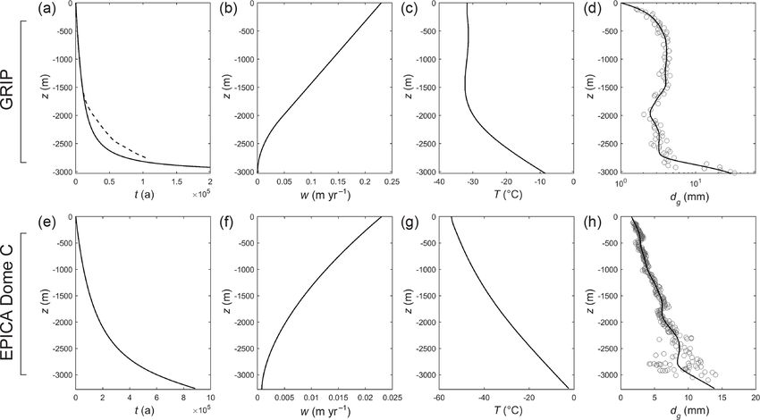
Figure 4. Ice-core background fields used in our signal evolution experiments. GRIP ice core: (a)–(d). (a) Age–depth scale and (b) ice
velocity from a Dansgaard–Johnsen model. Dashed line in (a) shows the GICC05 modelext timescale (Seierstad et al., 2014; Rasmussen
et al., 2014). (c) Ice temperature from Johnsen et al. (1995). (d) Grain-size data from Thorsteinsson et al. (1997) and spline fit used in
our modelling. EPICA Dome C core: (e)–(h). (e) Age–depth scale and (f) ice velocity from the model described in Sect. 3.1. (g) Borehole
temperature from Pol et al. (2010). (h) Grain-size data from Durand and Weiss (2004) and spline fit used in our modelling.
al. (2001) argued that |cB (∂wc /∂z)|
|wc (∂cB /∂z)|, but we 3.2 Results: single-peak experiments
do not ignore the term −cB (∂wc /∂z0 ) on the right-hand side
of Eq. (30), because the full flux divergence ∂(wc cB )/∂z0 is
Figure 5a presents snapshots from a GRIP run of the evo-
needed for solute conservation, i.e. no leakage.
lution of a decimetre-scale signal doped as a Gaussian peak
We experiment with two sets of background profiles
(grey curve: cB = 1 + 5 exp[−(z0 /1)2 ], with 1 = 0.08 m) in
(Fig. 4), based on the glaciological conditions at the GRIP
ice 500 years old (z = 112.4 m). Initially the peak, centred
ice-core site in central Greenland and the EPICA Dome
at z0 = 0, has a “full width at half maximum” (FWHM) of
C core site in Antarctica. In the GRIP runs, we use the
0.13 m. Its set amplitude, 5 µM, is based on the size of com-
depth–age scale t (z) and velocity w(z) from a Dansgaard–
monly observed peaks in ice-core records (e.g. ∼ 600 µg L−1
Johnsen model with the ice thickness H = 3029 m, the
for SO2−
4 ; ∼ 150 µg L
−1 for Cl− ; ∼ 80 µg L−1 for Na+ ). The
kink at 1000 m above the bed, and surface accumulation
peak decays rapidly in the first 20 kyr (upper 2 km at the
rate a = 0.23 m yr−1 ice equivalent. In the EPICA runs,
GRIP site) with negligible migration and migrates into z0 >
we use t (z) and w(z) from the model w = mbase + (a −
0 more noticeably afterwards, as the ice section descends
mbase )[(H − z)/H )]n (Ritz, 1992) with H = 3275 m, n =
deeper where the temperature gradient increases (Fig. 4c).
1.7, a = 0.023 m yr−1 , and the basal melt rate mbase =
Movie S1 shows the full evolution of this control run. Strong
0.0008 m yr−1 , which yields a depth–age scale approximat-
diffusion of the signal is evident not just from the peak’s de-
ing the one published by Parrenin et al. (2007). Smoothed
cay, but also from its broadening, which overcomes the effect
versions of T (z) and dg (z) measured at the ice-core sites
of vertical compression. Recall that in the material reference
are used (Fig. 4c–d, g–h). The prescribed profiles are ex-
frame, compression shortens the section continually, so ice
emplative only. In reality, ice at different depths has expe-
enters the simulation domain at both ends. Figure 5b and c
rienced different glaciological conditions due to changing
exemplify the perturbation on c (caused by the cB peak) and
accumulation, ice-sheet elevation, and climatic temperature
the resulting large wiggle on the velocity wc , which repre-
over interglacial–glacial timescales. Our interest is not in re-
sents the γ contribution in Eq. (22) and is what causes the
constructing the histories of these conditions.
Gibbs–Thomson diffusion. As in Rempel’s theory, the sig-
https://doi.org/10.5194/tc-15-1787-2021 The Cryosphere, 15, 1787–1810, 20211796 F. S. L. Ng: Pervasive diffusion of climate signals recorded in ice-vein ionic impurities Figure 5. Modelled evolution of a signal peak in (a)–(c) the GRIP control run and (d)–(f) an otherwise identical run where the Gibbs– Thomson effect is turned off (γ = 0). Snapshots are shown in the material reference frame, with displacement z0 measuring how far the signal has moved from ice of the same age (which lies at z0 = 0). (a, d) Bulk solute concentration cB ; (b, e) vein solute concentration c at one time; (c, f) anomalous velocity wc , porosity φ, and vein curvature rv at one time. Grey curves in (a) and (d) indicate the initial doped peak. Panel (b) illustrates the Gibbs–Thomson perturbation. See Movie S1 for the full simulations. nals on φ and rv are collocated with the cB peak throughout Figure 6a–c and Movie S2 present the control run for the evolution. EPICA, where ice 4 kyr old (z = 89.9 m) is doped with the To check this diagnosis for the origin of signal diffusion, same peak. The simulated behaviour is similar to that in the another run is conducted (Fig. 5d–f; Movie S1) with ev- GRIP run, but occurs on a much longer timescale due to the erything unchanged except that the Gibbs–Thomson term in low accumulation rate at the EPICA site. The peak migrates Eq. (5) is turned off by setting γ = 0. As expected, the strong from the start because a sizeable temperature gradient spans diffusion in the control run disappears, as no perturbation the ice column (Fig. 4g). Low compressive strain rate, cou- now arises on c and wc , but there is still residual diffusion pled with slow ice submergence and long time for diffusion, from vein motion. The peak narrows under vertical compres- yields a wider peak at all depths than in the GRIP run that has sion without much amplitude reduction until t ≈ 20 kyr. It a vastly increased “age span” (i.e. the peak’s width in the age subsequently decays because strong cB gradients on its steep- domain; discussed later in Fig. 8c, f) compared to the doped ening sides amplify the residual diffusion, despite κ being signal. Again, comparison against a run with γ = 0 (Fig. 6d– small (∼ 10−8 m2 yr−1 ; Fig. B2). The peak’s migration tra- f; Movie S2) confirms the Gibbs–Thomson perturbation as jectory in this run is identical to that in the control run be- the cause of signal damping and broadening and illustrates cause migration is independent of the peak shape and the the weaker residual diffusion. diffusion mechanisms. By t ≈ 100 kyr (≈ 2800 m depth) it The rapidity of signal widening versus migration in dis- has displaced from the ice by ≈ 0.6 m. A further experi- torting the peak in both control runs (Figs. 5a and 6a) is antic- ment with κ = γ = 0 (not shown) reproduces the “Rempel ipated by the non-small dimensionless number χ in Sect. 2.5. limit” of a migrating peak with no diffusion, as far as its According to Eq. (24), near-constant temperature in the top diminishing width can be resolved by our z0 -grid spacing, half of the GRIP column (Fig. 4c) preconditions a large 0.0025 m. This implies that the simulated signal behaviour χ there. Indeed, signal diffusion dominates that part of the in the experiments is not due to numerical diffusion in our GRIP control run, also confirming its independent operation finite-difference scheme. Finally, repeating the control run from migration. Deeper in both cores, migration becomes with κ = 0 modifies the results in Fig. 5a only slightly, con- more significant as χ is reduced by higher T and higher firming that residual diffusion becomes important only when dT /dz. In theory, larger grain sizes near the bed (Fig. 4d, h) a signal becomes very narrow. also slow the rate of the simulated signal decay, but the peaks The Cryosphere, 15, 1787–1810, 2021 https://doi.org/10.5194/tc-15-1787-2021
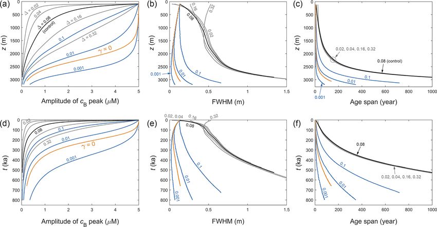
F. S. L. Ng: Pervasive diffusion of climate signals recorded in ice-vein ionic impurities                                                   1797

Figure 6. Modelled evolution of a signal peak in (a)–(c) the EPICA control run and (d)–(f) an otherwise identical run where the Gibbs–
Thomson effect is turned off (γ = 0). (a, d) Bulk solute concentration cB ; (b, e) vein solute concentration c at one time; (c, f) anomalous
velocity wc , porosity φ, and vein curvature rv at one time. Grey curves in (a) and (d) indicate the initial doped peak. Panel (b) illustrates the
Gibbs–Thomson perturbation. See Movie S2 for the full simulations.

in our control runs have long dissipated before reaching such              (grey curves). The control runs (black) and the runs where the
depths.                                                                    Gibbs–Thomson effect has been turned off (orange) are in-
   These initial runs demonstrate the signal migration of                  cluded for comparison. As shown by the grey curves, doping
Rempel’s theory, but paradoxically highlight that signals may              a narrower initial peak hampers its survival, as its steep sides
not survive deep into the ice where it predicts their displace-            cause strong diffusional draw-down of amplitude; broader
ment to become so large to be palaeoclimatically important.                peaks retain amplitude for longer but meet the same fate
More precisely, some remnant signals always survive, but                   as they narrow under vertical compression. We observe an
with such small amplitudes and such large age spans com-                   interesting feedback between width and amplitude evolu-
pared to the original signals that all essential palaeoclimatic            tion. Compression steepens the flanks of signals to acceler-
information has been lost. There is an apparent problem to                 ate their damping, whereas amplitude reduction makes them
resolve, as distinct deep ionic peaks are found in many ice                shallower and less prone to damping and broadening. Thus
cores (Fig. 1) (e.g. Röthlisberger et al., 2008; Traversi et al.,          the compressive strain rate is a key driver of signal diffusion.
2009; Svensson et al., 2013; Tison et al., 2015; Schüpbach                 The balance of compression and broadening causes different
et al., 2018), although they may be due to impurities outside              peaks to end on similar width trajectories at depth (panels b
veins.                                                                     and e, Figs. 7 and 8). Accordingly, peaks with different initial
   Sticking with the vein model for now, can peaks with a dif-             time durations acquire near-equal age spans increasing down
ferent shape survive damping and broadening to reach deep                  core (panels c and f, Figs. 7 and 8), which define the mini-
ice? We study this by changing the width of the doped peaks,               mum time resolution for deep climate signals. These interac-
as this alters their flank gradient, which is a key control of             tions are absent from the study of Rempel et al. (2001), who
their diffusion rate. Sensitivity experiments are conducted by             did not simulate signal shape evolution. Their companion pa-
varying the width parameter 1 of the Gaussian function be-                 pers (Rempel et al., 2002; Rempel and Wettlaufer, 2003) did
tween 0.02 and 0.32 m (with the control run parameters un-                 so but excluded layer thinning and diffusion.
changed), and by tracking the amplitude, FWHM (full width                     So, can single peaks survive into deep ice? The 1 ex-
at half maximum), and age span of the peak in each simula-                 periments show that peaks at the decimetre or centimetre
tion. The age span is found by dividing the FWHM by the                    scale struggle to do so. Even for initially wide peaks (e.g.
local ice velocity w.                                                      1 = 0.32 m) near the firn–ice transition, the Gibbs–Thomson
   Figures 7 and 8 plot – for GRIP and EPICA, respectively                 diffusion has reduced their amplitude 4-fold by the time they
– the evolving peak morphometry in these “1 experiments”                   reach z ≈ 2300 m at GRIP (where the age is ≈ 25 ka) and

https://doi.org/10.5194/tc-15-1787-2021                                                            The Cryosphere, 15, 1787–1810, 2021
1798                                    F. S. L. Ng: Pervasive diffusion of climate signals recorded in ice-vein ionic impurities

Figure 7. Changing morphometry of the signal peak – its amplitude, full width at half maximum (FWHM), and age span – in the GRIP ice
core for different model parameters, plotted against depth (a–c) and age of the ice (d–f). Black curves plot the control run of Fig. 5a, and
orange curves plot the γ = 0 run of Fig. 5d. Grey curves plot the results of altering the width parameter 1 of the doped peak from 0.08
(control) to four other values. Blue curves plot the outcomes of suppressing molecular diffusivity D in the control run by the multiplicative
factors 0.1, 0.01, and 0.001 to simulate vein blockage. Parameter labels use the same colours as the curves. Peak width becomes difficult to
measure as amplitude diminishes, explaining the jittery appearance of some curves at depth.

Figure 8. Changing morphometry of the signal peak – its amplitude, full width at half maximum (FWHM), and age span – in the EPICA
ice core for different model parameters, plotted against depth (a–c) and age of the ice (d–f). Black curves plot the control run of Fig. 6a, and
orange curves plot the γ = 0 run of Fig. 6d. Grey and blue curves document the same sensitivity tests as conducted for the GRIP core (see
Fig. 7 caption for details). The FWHM and age-span axes are scaled to focus more on the blue and orange curves, rather than the deep ends
of the grey/black curves, as the corresponding signal amplitudes decay to near zero.

The Cryosphere, 15, 1787–1810, 2021                                                             https://doi.org/10.5194/tc-15-1787-2021
F. S. L. Ng: Pervasive diffusion of climate signals recorded in ice-vein ionic impurities                                                  1799

Figure 9. Modelled displacement z0 pk and age offset 1tpk of signal peaks (from ice of the same age) at the (a, b) GRIP and (c, d) EPICA
core sites for different parameters, plotted against depth and age of the ice. “Control” labels the control runs in Figs. 5a and 6a; 0.1 and 0.01
label those runs in Figs. 7 and 8 where the molecular diffusivity D is suppressed by these factors to simulate vein blockage. The control
curve in panel (a) is equivalent to the curve in Fig. 4 of Rempel et al. (2001), except these authors assumed a different age–depth scale from
ours.

2000 m at EPICA (≈ 175 ka). Setting γ = 0 prolongs the sig-                ure 9 shows that in the control runs the peaks displace by
nals’ survival (Figs. 5–8), but residual diffusion still prevents          ∼ 1 m or more in deep ice, causing their apparent age to
them from reaching the lowest several hundred metres with                  exceed their true age by hundreds of years in ice ≈ 100 ka
a sizeable fraction of their original amplitude, not to mention            at GRIP, and by several thousand years in ice ≈ 500 ka at
that ignoring the Gibbs–Thomson effect is unphysical.                      EPICA. Since the migration rate is independent of the sig-
   In the present theoretical framework, is there any way for              nal shape, the 1 experiments yield the same displacements
signals to reach deep ice without losing integrity (ampli-                 and offsets as the control experiments. For both sets of ex-
tude, narrowness)? One possibility is the suppression of so-               periments, Figs. 7 and 8 (panels c and f) show that peaks
lute transport by partial vein blockage/disconnection, which               arriving in deep ice have age spans of several hundred years
we simulate here in a crude manner by artificially decreasing              at GRIP and several thousand years at EPICA (approaching
the molecular diffusivity D – this cannot capture heteroge-                the precession timescale in ice 700–800 kyr old); however,
neous vein transport at the grain scale. In Figs. 7 and 8, the             we caution against using these results to evaluate deep cli-
blue curves plot the results of simulations with D suppressed              matic histories retrieved from ice cores, because these sets
by different factors. The same doped peak and parameters of                of experiments predict near-zero signal amplitude at such
the control runs are used otherwise. A suppression factor of               depths. In contrast, decreasing D suppresses both signal mi-
0.001–0.01 postpones signal decay to a similar extent as turn-             gration and diffusion (see Eq. 23), so the corresponding
ing off the Gibbs–Thomson effect. The lesser factor (0.001)                peaks remain much narrower during their evolution (Figs. 7
allows the peak to reach 2750 m with half its original am-                 and 8, panels b and e) and migrate much less than in the
plitude. Even with such strong suppression, however, peak                  control/1 runs (Fig. 9, numbered curves). A suppression fac-
survival is hindered in deeper ice because the low strain rate             tor of 0.001–0.01 enables a peak with FWHM < 0.2 m, age
there (Fig. 4b, f) provides ample time for signal diffusion to             span < 200 yr, and potentially detectable amplitude to reach
occur, and because rising temperature near the bed increases               ≈ 2900 m depth, with an age offset of < 50 yr at GRIP and
κ. Note that in Figs. 7 and 8, a perfectly preserved peak sig-             < 300 yr at EPICA. These numerical findings are illustra-
nal that does not diffuse would have constant amplitude and                tive, as they depend on the depth–age scale assumed for each
age span, and its FWHM would decrease towards the bed as                   site (notably its precise behaviour at depth) and are limited
a result of vertical compression.                                          by the fact that we are not solving the inverse problem with
   The simulated displacement, age offset, and age span of                 time-varying palaeoclimatic forcing. Using them to interpret
the peaks are of potential palaeoclimatological interest. Fig-             specific details of the ice-core records is not advisable at this

https://doi.org/10.5194/tc-15-1787-2021                                                            The Cryosphere, 15, 1787–1810, 2021
1800                                  F. S. L. Ng: Pervasive diffusion of climate signals recorded in ice-vein ionic impurities

                                                                      by adding many Gaussian peaks (numbering 300 at GRIP
                                                                      and 1200 at EPICA) of random amplitudes, widths, and po-
                                                                      sitions onto a 1 µM base level (Fig. 11a). Movies S4 and S5
                                                                      document these runs.
                                                                         We focus our analysis on the EPICA runs (Fig. 11;
                                                                      Movie S5), as the GRIP findings are qualitatively similar (al-
                                                                      though things occur faster there). In the control run (black
                                                                      curves), strong damping and merging smooth the signals
                                                                      rapidly, so cB (z0 ) retains long-scale variations only – and
                                                                      no peaks – at depth. This outcome is consistent with what
                                                                      we learned from the single-peak experiments. When D is re-
                                                                      duced (blue and red curves), compressional shortening, with
                                                                      the now slower diffusion, causes a bundle of peaks to merge
Figure 10. Snapshots (at four times) of the evolution of two neigh-
bouring peaks in a GRIP run that uses the control parameters of the
                                                                      into new signals that subsume their solute content. This pro-
run in Fig. 5a. Diffusional spreading causes the peaks to merge as    cess operates continuously on all signals, with stretches hav-
they approach each other under vertical compression. See Movie S3     ing a high density of peaks turning into peaks and stretches
for the full simulation.                                              having a low density turning into troughs. The vertical com-
                                                                      pression is crucial in helping signals maintain their integrity
                                                                      against diffusion.
stage because how much matrix or grain-boundary impurities               When D is suppressed by 0.03 (Fig. 11, red curves), we
contribute to those records is also unknown (Sect. 4).                see distinct peaks persisting in deep ice, many traceable back
   For completeness, all of the above experiments have been           in time to predecessor groups of peaks, rather than a single
repeated with doped peaks with twice the amplitude (10 µM),           peak (e.g. dashed boxes). The balance of diffusion and short-
to cater for some especially high (rarer) peaks in the observed       ening here is such that the deep peaks have similar widths
records, which may have more chance to survive. Although              as their shallow counterparts (∼ dm), despite an overall re-
the corresponding remnant signals retain greater bulk con-            duction of signal amplitude with depth. The ice in Fig. 11d
centrations at all depths than before, their pattern of decay         has shortened by approximately a factor of 10 since the start
relative to the initial amplitude and the FWHM and age span           of the run, so each peak there encapsulates the signals and
results are only marginally altered (Figs. S1 and S2 – see            solute of an original interval some 10 times longer. Signal
Supplement; cf. Figs. 7 and 8). Our single-peak experiments           survival here is aided by the enhanced survival of single
thus confirm the difficulty for palaeoclimate information to          peaks due to decreased molecular diffusivity (Sect. 3.2), but
be preserved at depth when the veins are connected.                   also involves the lumping of solute from neighbouring peaks.
                                                                      We find in further experiments (not shown) that when D is
3.3    Results: multiple-peak experiments                             reduced even more (suppression factor . 0.001), the peaks
                                                                      continue to narrow into the centimetre range at depth. Fig-
The diffusion of cB means that neighbouring peaks can                 ure 11 shows an effect known from the single-peak experi-
merge as they descend the ice column. This process is il-             ments: a decrease in D reduces signal displacement as well
lustrated in Fig. 10 and Movie S3 by a simulation with two            as signal broadening.
peaks. Their merging begins at ≈ 7 kyr; the deeper peak                  The foregoing experiments demonstrate how long-scale
moves towards z0 = 0 due to vertical ice compression; a bi-           averages on cB at shallow depths – reflecting long-term back-
modal signal ceases at ≈ 12 kyr. Such merging suggests a              ground levels of impurity input at an ice-core site – evolve
second explanation for why distinct peaks can feature in deep         to become meaningful variations at depth, as signals are
ice even with strong damping: instead of deriving from a sin-         compressed and their fine details filtered out by diffusion.
gle peak high up in the column, a deep peak might form                In Fig. 11, the mean level of the 3600-year-long signal se-
by the agglomeration of multiple signals or peaks as these            quence is preserved at depth as a bump (of the same duration)
merge under compression. This signal-forming mechanism                about 7 µM above the surrounding ice. Ice-core analyses of
may not be evident from the cB profile measured from ice              the major ions frequently interpret deep features of this kind
cores, which gives an instantaneous record of the signals.            as reflecting real palaeoclimatic variations on timescales of
   To test this idea, in the next experiments we simulate the         101 –102 kyr (e.g. Mayewski et al., 1997; Wolff et al., 2006;
evolution of multiple signals doped in shallow ice stretches          Schüpbach et al., 2018); it is understood that fewer high-
20 m long at GRIP and 80 m long at EPICA. Three runs are              frequency palaeoclimatic details are retrievable from deeper
made for each site, one with the control-case parameters and          ice, due to the finite resolution of ice-core sampling, along-
two with D suppressed by 0.1 and 0.03 (to simulate vein               side layer thinning, which causes more time to be encapsu-
blockage), with both the Gibbs–Thomson effect and resid-              lated in a given ice thickness. Our simulations highlight the
ual diffusion included, and using an initial cB profile formed        Gibbs–Thomson effect in vein impurity transport as a further

The Cryosphere, 15, 1787–1810, 2021                                                      https://doi.org/10.5194/tc-15-1787-2021
You can also read