Determination of the emission rates of CO2 point sources with airborne lidar
←
→
Page content transcription
If your browser does not render page correctly, please read the page content below
Atmos. Meas. Tech., 14, 2717–2736, 2021
https://doi.org/10.5194/amt-14-2717-2021
© Author(s) 2021. This work is distributed under
the Creative Commons Attribution 4.0 License.

Determination of the emission rates of CO2 point sources
with airborne lidar
Sebastian Wolff1 , Gerhard Ehret1 , Christoph Kiemle1 , Axel Amediek1, , Mathieu Quatrevalet1 , Martin Wirth1 , and
Andreas Fix1
1 Deutsches   Zentrum für Luft- und Raumfahrt (DLR), Institut für Physik der Atmosphäre, Oberpfaffenhofen, Germany
 deceased,   28 January 2021

Correspondence: Sebastian Wolff (sebastian.wolff@dlr.de)

Received: 27 September 2020 – Discussion started: 12 November 2020
Revised: 5 February 2021 – Accepted: 19 February 2021 – Published: 8 April 2021

Abstract. Anthropogenic point sources, such as coal-fired        dars are intrinsically independent of sunlight, they have a
power plants, produce a major share of global CO2 emis-          significant advantage in this regard.
sions. International climate agreements demand their in-
dependent monitoring. Due to the large number of point
sources and their global spatial distribution, the implemen-
tation of a satellite-based observation system is convenient.    1   Introduction
Airborne active remote sensing measurements demonstrate
that the deployment of lidar is promising in this respect.       CO2 causes the strongest radiative forcing among all anthro-
The integrated path differential absorption lidar CHARM-F        pogenic greenhouse gases (GHGs; e.g., Myhre et al., 2014).
is installed on board an aircraft in order to detect weighted    Therefore, it plays a crucial role with respect to human-
column-integrated dry-air mixing ratios of CO2 below the         induced climate change. In 2018, CO2 reached a global an-
aircraft along its flight track. During the Carbon Dioxide and   nual average of 407.4 ppm at the Earth’s surface, an increase
Methane Mission (CoMet) in spring 2018, airborne green-          of 47 % compared to the year ∼ 1750 (Friedlingstein et al.,
house gas measurements were performed, focusing on the           2019). One third of all anthropogenic CO2 emissions stem
major European sources of anthropogenic CO2 emissions,           from localized point sources, in particular coal-fired power
i.e., large coal-fired power plants. The flights were designed   plants (Oda and Maksyutov, 2011). For Europe, they even
to transect isolated exhaust plumes. From the resulting en-      account for 45 % of CO2 emissions (Super et al., 2020). The
hancement in the CO2 mixing ratios, emission rates can           Paris Climate Agreement aims to reduce anthropogenic GHG
be derived via the cross-sectional flux method. On average,      emissions by means of nationally determined contributions
our results roughly correspond to reported annual emission       (NDCs) which are based on national capabilities and the level
rates, with wind speed uncertainties being the major source      of economic development (UNFCCC, 2015). Therein it is
of error. We observe significant variations between individ-     foreseen that as of 2023 a global stocktake will take place
ual overflights, ranging up to a factor of 2. We hypothesize     every 5 years. This requires independent measurements to
that these variations are mostly driven by turbulence. This      verify each nation’s emission reports of CO2 but also of other
is confirmed by a high-resolution large eddy simulation that     greenhouse gases, such as CH4 . Currently, there is no inde-
enables us to give a qualitative assessment of the influence     pendent global emission verification system available, and
of plume inhomogeneity on the cross-sectional flux method.       a complete record of all emissions globally is still far from
Our findings suggest avoiding periods of strong turbulence,      reality. To achieve this goal, satellite missions are indispens-
e.g., midday and afternoon. More favorable measurement           able. Satellite missions are expected to detect CO2 emissions
conditions prevail during nighttime and morning. Since li-       from large power plants and cities, e.g., the future European
                                                                 carbon constellation CO2M (Bézy et al., 2019; Broquet et al.,
                                                                 2018; Kuhlmann et al., 2020) and other mission ideas still

Published by Copernicus Publications on behalf of the European Geosciences Union.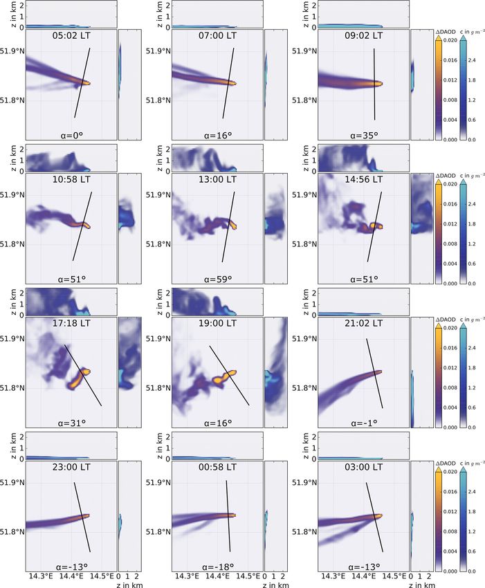
2718                          S. Wolff et al.: Determination of the emission rates of CO2 point sources with airborne lidar

in the pre-development phase (Kiemle et al., 2017; Strand-           lidar approach. Albedo variations basically affect the mea-
gren et al., 2020). Furthermore, CH4 emissions can also be           surement precision (statistical uncertainty), whereas the in-
detected, as is done by GHGSat-D for coal mine ventilation           fluence on the bias is negligible (Amediek et al., 2009).
shafts (Varon et al., 2020) or the Sentinel-5 Precursor for the         During the CoMet campaign, HALO probed various local
oil- and natural-gas-producing sector (Pandey et al., 2019;          plumes of different coal-fired power plants. As a case study,
Zhang et al., 2020). Under particularly favorable conditions,        the paper in hand focuses on the measurement flight of 23
it is already possible to detect CO2 emissions of power plants       May 2018, in which the CO2 exhaust plume of the power
from space, as is done with data from NASA’s OCO-2 mis-              plant Jänschwalde, close to the Polish–German border, was
sion (Nassar et al., 2017; Reuter et al., 2019). However, at         surveyed. The specific goal is to quantify the CO2 fluxes
the moment no operating satellite mission is able to quan-           of the power plant. An established method for quantifying
tify emissions from large power plants on a regular basis. In        emission rates of point sources is the cross-sectional flux
the development phase for potential missions, airborne mea-          method, which is a product of mean wind speed and an in-
surement campaigns serve as a test of the methods. During            tegrated concentration enhancement along a cross-sectional
the operating phase, they are needed for verification of the         overflight of the exhaust plume. This principle has been ap-
space-borne results.                                                 plied to air- and space-borne nadir-viewing remote sensing
    In May/June 2018, the CoMet (Carbon Dioxide and                  (Krings et al., 2018; Menzies et al., 2014; Varon et al., 2018;
Methane Mission) field campaign took place. The objective            Reuter et al., 2019), mobile ground-based sun-viewing re-
of CoMet was to investigate the fluxes of the major human-           mote sensing (Luther et al., 2019), and airborne in situ mea-
influenced GHGs on local, regional, and sub-continental              surements (Cambaliza et al., 2014; Conley et al., 2016; Fiehn
scales. These fluxes were to be determined more precisely            et al., 2020; White et al., 1976). Amediek et al. (2017) have
than previously possible. Furthermore, supporting activities         described how this principle can be realized with CHARM-
for GHG stocktaking were provided. The CoMet campaign                F. Using CHARM-F data from the respective overflights, we
saw the deployment of a suite of airborne instruments to             strive to accurately assess the error and advance the general
measure atmospheric CH4 and CO2 , alongside a variety of             methodology.
ground-based instruments. In particular, the synergetic use             When determining the cross-sectional flux, one of the ma-
of active remote sensing (lidar) (Amediek et al., 2017; Wild-        jor error sources is the local wind field: on the one hand,
mann et al., 2020), passive spectrometry (Krautwurst et al.,         because the wind speed is directly included in the calcula-
2021; Luther et al., 2019), and in situ measurements (Fiehn          tion, on the other hand, because atmospheric turbulence can
et al., 2020; Gałkowski et al., 2021; Kostinek et al., 2020)         broaden or constrict the spatial extent of the exhaust plume.
supported by modeling activities (Chen et al., 2020; Nickl et        This is a well-known problem which contributes significantly
al., 2020), as well as the validation of existing (e.g., Sentinel-   to the measurement error (Kuhlmann et al., 2019; Luther et
5P, GOSAT, Greenhouse gases Observing SATellite) and the             al., 2019; Strandgren et al., 2020; Varon et al., 2018; Jon-
preparation of upcoming (e.g., MERLIN, MEthane Remote                garamrungruang et al., 2019; Kumar et al., 2020). Conse-
sensing Lidar missioN) GHG satellite missions, was aimed             quently, the observed CO2 column enhancements between
at.                                                                  subsequent plume transects may vary considerably despite a
    Hereby, the German research aircraft HALO (High Alti-            constant emission rate. We hypothesize that these turbulence-
tude and Long Range Research Aircraft) acted as the air-             induced variations dominate the measurement error of the
borne flagship of that campaign. HALO was equipped with              emission estimates rather than the GHG column measure-
the new airborne CO2 and CH4 IPDA (integrated path dif-              ment uncertainty itself. To assess the impact of this atmo-
ferential absorption) lidar CHARM-F (CO2 and CH4 Atmo-               spheric turbulence on our measurement results, we perform a
spheric Remote Monitoring Flugzeug) built and operated by            large eddy simulation (LES) in order to resolve local plume
DLR as an airborne demonstrator of the upcoming MERLIN               structures. By doing so, we can compare different ambient
mission (Ehret et al., 2017). CHARM-F simultaneously mea-            weather and turbulence conditions. We aim to separate more
sures the column-averaged dry-air mixing ratios of carbon            and less favorable conditions, to determine an adequate dis-
dioxide (XCO2 ) and methane (XCH4 ) between the aircraft             tance between emission source and measurement locations,
and ground (Amediek et al., 2017). The influence of other            and to find out how many independent plume measurements
trace gases, in particular H2 O, on the mixing ratio measure-        will be necessary in order to obtain an appropriate emission
ments is negligible. As a result of the pulse repetition fre-        rate accuracy as a function of those environmental condi-
quency (50 Hz, double pulse) and divergence (∼ 1.5 mrad),            tions.
the pattern on the ground is a sequence of overlapping foot-            This paper is organized as follows. Section 2 introduces
prints. The vertical column measurements are insensitive to          the IPDA lidar method and describes the retrieval of the
the vertical redistribution of the trace gases. The insensitiv-      emission rate and the methodical errors. Section 3 reports
ity towards optically thin clouds, aerosol layers, and varying       on the plume measurement results. Section 4 provides the
surface albedo, and the instrument design with, e.g., active         simulation setup, while the subsequent results are presented
laser frequency control, is a further strong asset of the IPDA

Atmos. Meas. Tech., 14, 2717–2736, 2021                                               https://doi.org/10.5194/amt-14-2717-2021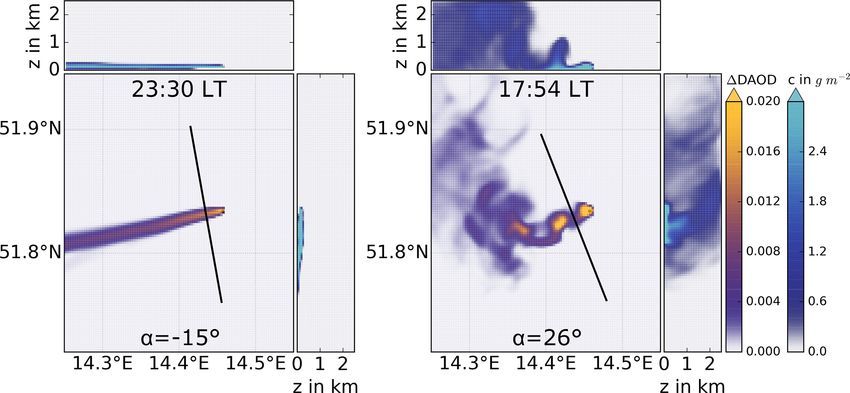
S. Wolff et al.: Determination of the emission rates of CO2 point sources with airborne lidar                                        2719

in Sect. 5. A discussion is given in Sect. 6, followed by the
conclusion in Sect. 7 and the outlook in Sect. 8.

2     Cross-sectional flux method

2.1    Flux calculation

The dataset underlying this work originates from the IPDA
lidar CHARM-F. A more detailed description of the lidar
system can be found in Amediek et al. (2017). At its core,
CHARM-F consists of a pulsed, tunable laser source and
a detector. Installed on an aircraft or satellite, the nadir-
oriented lidar emits two laser pulses that propagate through
the atmosphere until they are backscattered at a surface. The
two backscattered laser pulses are detected by the lidar. The
wavelength of one laser pulse corresponds to the absorption
wavelength of the greenhouse gas under consideration. In the
following, this laser pulse is referred to as online. Due to
molecular absorption, the intensity of the online laser pulse
decreases while propagating through the atmosphere. The
wavelength of the other (offline) laser pulse is slightly shifted
such that almost no absorption by the greenhouse gas takes
place, but the interaction with the remaining atmospheric
components is unaltered.
   Using a beam splitter, a small part of both the online and
the offline laser pulse energy (Eon/off ) is deflected onto a de-
tector while still in the lidar system. Together with the radia-
tion fluxes entering the lidar telescope Pon/off , the differential
optical absorption depth (DAOD) can be calculated (Ehret et
al., 2008).

            1       Poff /Eoff
DAOD = · ln                                                    (1)
            2       Pon /Eon

Note that for the DAOD a single value is obtained for the
entire vertical air column. It is a metric for the greenhouse
                                                                      Figure 1. Figure by Amediek et al. (2017). The measurement geom-
gas concentration of the measured column and is also defined
                                                                      etry of a lidar, illustrated by the example of CHARM-F carried on
by the following relationship.                                        the aircraft HALO. Two laser pulses are emitted towards the earth
                                                                      with a delay of 500 µs. The laser pulse with the wavelength λon
DAOD = DAODb + 1DAOD                                           (2)    is on the absorption line of CO2 (1572.02 nm), and the laser pulse
                           Zfl                                        with the wavelength λoff is not (1572.12 nm). By comparing the
                    1                                                 backscattered intensities, the CO2 concentration in the measured
          = DAODb +                1σ (z) · 1c(z) dz
                    M                                                 cone volume can be calculated. The measured volume is usually re-
                           0                                          ferred to as a vertical air column since the column length, i.e., the
                               Zfl                                    aircraft’s altitude above ground (∼ 6500 m), is very large compared
                    1σ                                                to the diameter of the reflecting surfaces (∼ 10 m). The distance of
          ≈ DAODb +                  1c(z) dz
                    M                                                 consecutive laser pulse pairs is 3 m. The black line in (b) schemati-
                               0                                      cally depicts the measurement principle, not the actual spectral ab-
                                                                      sorption line shape of CO2 .
Here, DAODb is the background differential absorption opti-
cal depth, 1DAOD is the enhancement in the DAOD induced
by the plume, M is the molecular mass of CO2 in grams (g),
1c(z) is the enhanced CO2 density induced by the plume in             It is referred to as the differential absorption cross section.
grams per cubic centimeter (g cm−3 ), and 1σ (z) is the dif-          Generally, 1σ (z) is not constant over the plume’s vertical
ference between the CO2 absorption cross section for the two          extension due to the decreasing pressure with altitude. How-
laser wavelengths given in square meters (m2 ; cf. Fig. 1).           ever, the decreases in pressure associated with typical ver-

https://doi.org/10.5194/amt-14-2717-2021                                                 Atmos. Meas. Tech., 14, 2717–2736, 2021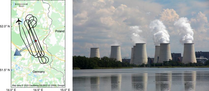
2720                          S. Wolff et al.: Determination of the emission rates of CO2 point sources with airborne lidar

tical plume extensions are small. As an approximation, we            The relative uncertainties
                                                                                               in these parameters are denoted by
use the mean value over the vertical extent of the plume.            δA/A, δ 1σ /δσ , and δu/u denote the relative uncertain-
This aspect is discussed in more detail in Sect. 3. The ver-         ties in these parameters. From this, it is obvious that crossing
tical integral limits are the ground (z = 0 m) and the respec-       the plume perpendicular to the wind direction as displayed
tive height of the aircraft flights (z = fl). Variations in flight   in Fig. 2a would give the highest accuracy for any fluctua-
altitude, as well as topography, may cause variations in the         tion in the wind direction δϕ. On the other hand, atmospheric
surveyed column length and thus ultimately in the measured           conditions at low wind speeds or situations with high atmo-
DAOD. In this study, these variations are negligible since the       spheric turbulence are in general less favorable because of
flight altitude was deliberately kept constant, and the topog-       the high uncertainty in the mean wind speed and wind di-
raphy around the power plant under consideration is suffi-           rection. Varon et al. (2018) have identified 2 m s−1 as the
ciently flat.                                                        minimum threshold of wind speed for the applicability of
   This DAOD dataset is used to determine the CO2 emis-              the cross-sectional flux method. This minimum value is also
sion rate of a point source utilizing the flux calculation           referred to by Sharan et al. (1996), arguing that above this
method introduced by Amediek et al. (2017). As schemat-              threshold, advection dominates over diffusion.
ically depicted in Fig. 2, a crossing of the exhaust plume
leads to a DAOD enhancement. This is caused by the ad-               2.2   Background separation
ditional absorption of laser radiation by the CO2 molecules
of the plume. The instantaneous flux through the lidar cross-        For the calculation of the integrated enhancement A and its
section, at the moment of the overflight, is given in kilograms      uncertainty, it is crucial to distinguish between the DAOD
per second (kg s−1 ) and denoted by q.                               value attributable to the background concentration of CO2
         M                                                           and the fraction attributable to the exhaust plume of the point
q = A·        · u · sin(ϕ)                                   (3)     source. As shown in Eq. (2), the measured DAOD along
         1σ
                                                                     the flight track is the sum of background term DAODb and
Given in meters (m), the parameter A corresponds to the in-          the enhancement due to the plume interaction (1DAOD). A
tegrated DAOD enhancement over the background DAOD in                complicating factor is that the background term may not be
the direction of the aircraft flight track as shown in Fig. 2b.      constant. There are small variations in local CO2 concentra-
In the following, it is referred to as integrated enhancement.       tion from other anthropogenic sources (traffic, cities, etc.) or
The mean horizontal wind speed u is given in meters per sec-         local interaction with the biosphere. Also, small CO2 gradi-
ond (m s−1 ), and the angle between the wind direction and           ents caused by the sounding of different air masses in the
the aircraft’s flight direction is denoted as ϕ (in the follow-      vicinity of the plume may have an impact on the background
ing referred to as relative wind direction). Furthermore, it         term. In the following, we describe a suitable method that en-
is assumed that no uptake by the soil takes place when the           ables us to extract 1DAOD from the measured dataset while
gas plume hits the ground and that the flight altitude is high       allowing the background term to be variable.
enough (i.e., well above the planetary boundary layer, PBL)             An example of the plume extraction procedure is shown
to cover the entire vertical extent of the plume.                    in Fig. 3. The plume must first be detected as an enhance-
   The two closely spaced sounding wavelengths are selected          ment not attributable to noise in the data. For this, we exam-
in such a way that the impact from unknown particles is min-         ine a 0.2 km running mean of the DAOD dataset (Fig. 3a).
imized while keeping the absorption by water vapor as low as         The choice of 0.2 km is made because it corresponds to the
possible. This is due to the very weak water vapor differen-         diameter of the pixels of the simulation (see Sect. 4). The
tial absorption cross section, which is more than 4 orders of        larger the window for the running mean is, the less noise is
magnitude smaller than the differential absorption cross sec-        present and the clearer the plume enhancement can be seen.
tion for CO2 . Thus, the influence of additional water vapor in      Then again, peaks threaten to be blurred if the window width
the plume released by the cooling or coal drying systems of          becomes too large.
the power plant is negligible (Kiemle et al., 2017). Moreover,          Starting from the middle of the plume enhancement, we
the selected CO2 absorption line is sufficiently temperature-        define the plume’s limits as the intersections between the
insensitive such that the influence of temperature variations        0.2 km running mean (RM) and another 4 km running mean
within the plume can be neglected (see also Kiemle et al.,           (Fig. 3b). Applying a running mean broadens and flattens
2017). Under these conditions, the flux error is mainly driven       the plume. For larger running mean widths, such as 4 km,
by uncertainties in the four parameters A, 1σ , u, and ϕ. As-        the flattening is so severe that the plume is only distinguish-
suming that these parameters are not correlated, the relative        able from the background as a raised plateau (see Fig. 3b).
accuracy in the flux calculation can then be estimated by er-        The limits are then defined as the intersections between the
ror propagation means.                                               0.2 and the 4 km running means. For the calculation of this
       v
       u                      !2                                 mean we consider a window with a width equal to that of
            δA 2                        δu 2
                                                        2
δq u                     δ(1σ )                     δϕ               the plume, colored violet in Fig. 3c. At last, we execute
     = t             +             +         +               (4)
 q          A              1σ            u        tan(ϕ)             another 4 km running mean over the raw dataset with by-

Atmos. Meas. Tech., 14, 2717–2736, 2021                                               https://doi.org/10.5194/amt-14-2717-2021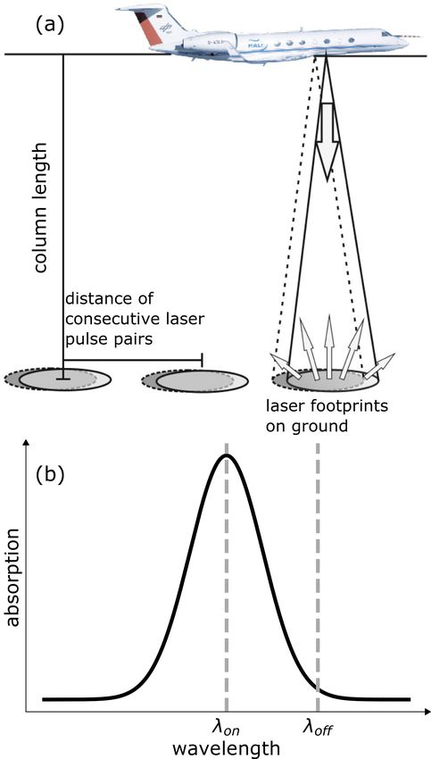
S. Wolff et al.: Determination of the emission rates of CO2 point sources with airborne lidar                                         2721

Figure 2. Crossing an exhaust plume illustrated by the example of CHARM-F carried on the aircraft HALO. (a) Two laser pulses are emitted
towards the earth with a short delay. The laser pulse with the wavelength λon is on the absorption wavelength of CO2 , and the laser pulse
with the wavelength λoff is not. By comparing the backscattered intensities, the DAOD can be calculated (see Sect. 2.1). An ideal exhaust
plume of a point source has a Gaussian-shaped mean concentration distribution both horizontally and vertically. (b) A perpendicular crossing
of the plume yields a Gaussian-shaped DAOD dataset.

passed plumes, resulting in the background term DAODb ,                 flight track. Both methods were investigated in the course of
shown in brown in Fig. 3d. This procedure allows for a vari-            this work and showed nearly identical results. Therefore, the
ability in the background term on a scale of a few hundred              results in Table 1 correspond to the mean value of the two
meters. Smaller scale gradients cannot be attributed to the             methods.
background and are incorporated in the enhancement term
1DAOD, thereby not being distinguishable from noise.
   The mean wind speed u and its mean relative direction                3   Airborne measurements
ϕ are extracted from model data provided by ECMWF. The
                                                                        In this work the measurement flight of HALO on 23 May
molecular mass M and the differential absorption cross sec-
                                                                        2018 between 10:24 and 11:36 CEST (Central European
tion 1σ are physical properties of CO2 and available in vari-
                                                                        summer time) is investigated. Located in the southeast of
ous databases such as HITRAN2016 (Gordon et al., 2017).
                                                                        the German federal state of Brandenburg close to the Polish–
The only parameter that results from a measurement by
                                                                        German border, the Lausitz Energie Kraftwerke AG (LEAG)
CHARM-F, or a respective simulation, is the integrated en-
                                                                        operates the coal-fired power plant Jänschwalde. It is one
hancement A. For this purpose Amediek et al. (2017) de-
                                                                        of the largest power plants in Europe both in terms of an-
scribed two distinct methods. The first method is a Riemann
                                                                        nual electricity generation and annual CO2 emissions. For the
sum over all enhancement values 1DAODi multiplied by
                                                                        year 2017, the power plant operators have reported an emis-
their respective spatial distance 1yi between two successive
                                                                        sion quantity of 24.0 Tg (CO2 ) to the European Environment
data points.
                                                                        Agency (E-PRTR, 2020). The exhaust gases of this power
           X
                               !                                        plant are emitted through the cooling towers at a height of
Asum =         1DAODi · 1yi                               (5)           ∼ 120 m. Figure 4 shows the flight track of the aircraft, along
            i                                                           with a picture of the cooling towers. In total, the point source
                                                                        was flown over seven times downwind, two times upwind,
The second method makes use of the fact that, on average, the
                                                                        and once directly over the cooling towers. In three of the
plume is subject to Gaussian dispersion behavior. According
                                                                        downwind overflights, no enhancement in DAOD is visible.
to the function F (y) in Eq. (6), a nonlinear least squares fit
                                                                        For these transects, the distance to the point source is greater
is applied to the 1DAOD values of the plume.
                                                                        than 4.6 km. At such distances, it can be assumed that the
            Afit

                               y−A1 2
                                                                       exhaust gases are too diluted with the surrounding air to gen-
                  −1·
F (y) =       √ ·e 2            A2
                                                               (6)      erate a measurable signal.
          A2 · 2π                                                          In order to evaluate the uncertainty of the calculated inte-
By doing so the integrated enhancement is obtained as the fit           grated enhancement, a total of 15 different data subsets cen-
parameter Afit . A1 is the peak’s position along the flight track       tered on the plume’s position, with varying width, are ex-
and A2 the turbulent dispersion parameter, which is a mea-              amined. To ensure that the Riemann sum completely covers
sure for the width of the plume. The fit method yields very             the plume, the smallest subset is twice as wide as the plume
low values for the uncertainty of the parameter A. However,             limits, determined according to Fig. 3. The width of the re-
the Riemann sum is not depending on any model assump-                   maining subsets is expanded by 400 m each.
tion for the calculation of the integrated 1DAOD along the

https://doi.org/10.5194/amt-14-2717-2021                                                   Atmos. Meas. Tech., 14, 2717–2736, 2021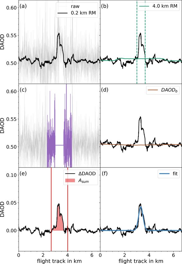
2722 S. Wolff et al.: Determination of the emission rates of CO2 point sources with airborne lidar
Table 1. Flight measurement results of individual crossings for the Jänschwalde power plant on 23 May 2018, following the nomenclature
of Eq. (3).
Crossing Measurement
Local Flight track Distance A 1σ q Mean q Mean u Mean ϕ
time (in km) (in km) (in m) (in 10−27 m2 ) (in kg(CO2 ) s−1 ) (in kg(CO2 ) s−1 ) (in m s−1 ) (in ◦ )
10:50 200 1.46 15.36 ± 0.67 7.27 ± 0.04 760 ± 60
10:57 268 4.77 9.04 ± 0.42 7.47 ± 0.24 470 ± 40
650 ± 240 5.06 ± 0.36 103.34 ± 6.40
11:10 388 1.67 19.29 ± 0.46 7.27 ± 0.04 950 ± 80
11:27 536 1.78 8.45 ± 1.11 7.27 ± 0.04 420 ± 40
To further evaluate Eq. (3), the differential absorption the lack of further information on turbulence characteristics
cross section 1σ is calculated using the Voigt-profile model during our measurements, we consider both plume widths in
with input from the HITRAN 2016 database for the line pa- the calculation below. The change in 1σ (z) versus altitude
rameters (Gordon et al., 2017). This calculation requires the above ground in Eq. (8) is calculated at grid cell spacing of
knowledge of pressure and temperature profiles, which are 1 m in the vertical direction using the following second order
extracted from the simulation introduced in Sect. 4. For the polynomial function.
lidar measurements, the online wavelength was tuned to the
CO2 absorption line center at λon = 1572.02 nm, while the 1σ (z) = 7.10652 × 10⁻²⁷ m2 (8)
offline wavelength was adjusted to λoff = 1572.12 nm in the + 8.60755 × 10 −31
m·z
wing of this line (cf. Fig. 1b). Based on this wavelength selec-
tion and a flight altitude of 8000 m, the background DAODb + 8.02673 × 10 −35
· z2
is approximately 0.5, while the plume causes a ∼ 10 % en-
hancement to this value (∼ 0.05), as depicted in Fig. 3. The Consequently, the differential absorption cross section at the
absorption cross section is not constant over the plume’s ver- height of the ground (70 m a.s.l.) corresponds to 1σ (z =
tical extension mainly due to the decreasing pressure and re- 0 m) = 7.10652 × 10⁻²⁷ m2 . The constant factors of this
sulting decrease in collisional line broadening with altitude. equation are the result of fitting this function to some repre-
The relative change in the absorption cross section along sentative cross-section values from Voigt-profile calculations
the vertical course of the plume depends on the exact on- over the altitude range of 4000 m. The deviations of this ap-
line position with respect to the absorption line center. To proximation to the exact Voigt-profile calculations are less
take a possible cross-section change for our measurements than 0.1 %, which is regarded as negligible. Finally, Eq. (7)
into account, representative mean values for the distances at gives the following results:
x1 ≈ 1500 and x2 ≈ 4700 m (see Table 1) are calculated us-
1σ (x1 = 1500 m) = 7.27 × 10⁻²⁷ m2 ± 0.04 × 10⁻²⁷ m2
ing the slender plume approximation (Amediek et al., 2017;
Seinfeld and Pandis, 1997). and
(z−h)2 (z+h)2
1σ (x2 = 4700 m) = 7.47 × 10⁻²⁷ m2 ± 0.24 × 10⁻²⁷ m2 .
− −
R max
1σ (z)·e
( (
2· σz x1,2 ))2 +e ( (
2· σz x1,2 ))2
dz
0
1σ x1,2 =
(z−h)2 (z+h)2
(7) The overscore indicates the mean value of the aforemen-
max − −
R ( (
2· σz x1,2
2
)) ( (
2· σz x1,2
2
)) tioned turbulence scenarios with corresponding plume ver-
e +e dz
0 tical widths at each distance, and the errors indicate the
differences. Close to the source (∼ 1500 m), the relative
In this equation, the ground (z = 0 m) and the maximum cross-section uncertainty is ∼ 0.6 % and therefore negligi-
(z = 4000 m) denote the integration boundaries, and h is the ble, whereas, at a distance of 4700 m, the relative error is
height of the cooling towers. The key parameter in this equa- ∼ 3.2 % and not negligible in the overall error budget out-
tion is the turbulence parameter σz , which is a proxy for the lined by Eq. (4).
plume extension in the vertical direction, at the respective Possible systematic errors due to uncertainties in the line
distance. Different expressions for this parameter for various parameters are less than 2 % (Gordon et al., 2017). Errors
atmospheric stability conditions can be found in the litera- resulting from the wavelength setting with the CHARM-F
ture, e.g., Seinfeld and Pandis (1997). instrument are considered very small compared to the other
Assuming a moderately turbulent atmosphere, we found contributors and therefore need not to be extensively dis-
plume widths of σz = 170 and 600 m for the two distances. cussed in this study (∼ 0.5 %; see Amediek et al., 2017).
However, if the atmospheric turbulence is less pronounced, The wind data are taken from operational analysis data of
the vertical plume widths are only σz = 90 and 250 m. Due to the ECMWF model. This is done by first interpolating the 4D
Atmos. Meas. Tech., 14, 2717–2736, 2021 https://doi.org/10.5194/amt-14-2717-2021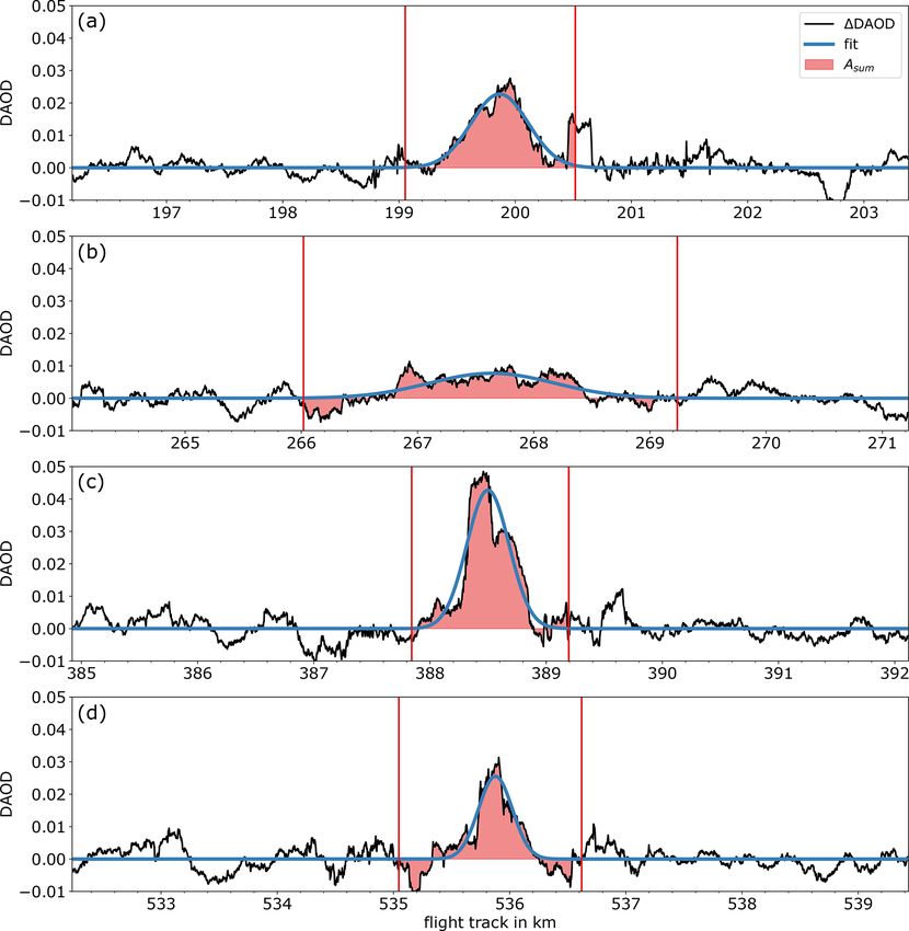
S. Wolff et al.: Determination of the emission rates of CO2 point sources with airborne lidar                                     2723

                                                                           Table 1 shows the measured integrated enhancements, the
                                                                        wind data, and the resulting fluxes for the four exploitable
                                                                        overflights, alongside the obtained mean values, under the
                                                                        assumption that during the measurement both the wind di-
                                                                        rection and the wind speed were reasonably constant. The
                                                                        flight segments were not exactly perpendicular to the mean
                                                                        wind direction. With a relative angle of ϕ = 103◦ a correc-
                                                                        tion factor of sin(103◦ ) = 0.97 is applied (see Eq. 3). The
                                                                        mean wind speed is well above the threshold of 2 m s−1 , in-
                                                                        troduced at the end of Sect. 2.1.
                                                                           The individual flux uncertainties, calculated with Eq. (4),
                                                                        are relatively small and range between 8 %–10 %. It is to be
                                                                        emphasized that the integrated enhancement A is the only pa-
                                                                        rameter in the calculation of the instantaneous flux in Eq. (3)
                                                                        coming from the IPDA lidar measurement itself. On average,
                                                                        2/10 of this individual measurement uncertainty is due to the
                                                                        uncertainty of the integrated enhancement δA/A. Taken to-
                                                                        gether, 1/10 can be attributed to the uncertainty of the mean
                                                                        differential absorption cross section of CO2 δ 1σ /δσ and
                                                                        the mean relative wind direction δϕ/ tan(ϕ). The major con-
                                                                        tributor to the flux uncertainty, however, is the uncertainty of
                                                                        the mean wind speed δu/u, which accounts for 7/10.
                                                                           The       reported      value      of       760 kg(CO2 ) s−1
                                                                                           −1
                                                                        (24.0 Tg(CO2 ) yr ) (E-PRTR, 2020) lies within the
                                                                        error range of the mean value of 650 ± 240 kg(CO2 ) s−1
                                                                        (20.3 ± 7.9 Tg(CO2 ) yr−1 ). Nevertheless, the variations
                                                                        between the individual crossings are very large, both in the
                                                                        integrated enhancement A and in the calculated fluxes. The
                                                                        second and third crossings differ by approximately a factor
                                                                        of 2 (see Table 1). These variations cannot be explained by
Figure 3. Plume crossing at a point source distance of 1.53 km. In
                                                                        our uncertainty estimation but rather by atmospheric turbu-
(a) the gray curve shows the raw data, with a standard deviation
                                                                        lence that distorts the plume. Therefore, this work further
of 5.2 %, while the black curve shows a 0.2 km (64 data points)
running mean (RM), with a standard deviation reduced to 0.9 %.          investigates the influence of atmospheric turbulence and
In (b) the green curve is a 4 km (1293 data points) RM. Vertical        the resulting inhomogeneity in the propagation of exhaust
dashed green lines mark the intersections between the 0.2 and 4 km      plumes. To achieve this, we make use of the mesoscale
RMs, which are defined as the plume’s limits. The color purple in       numerical weather prediction system model WRF (Weather
(c) shows the region of the data used to construct a mean value of      Research and Forecasting model).
the data before and after the plume’s limits. This mean value is used
to bypass the plume enhancement and is also colored purple. In (d)
again a 4 km running mean over the bypassed dataset is shown in         4   Simulation setup
brown. These data, which have slight variability, are used as the
background term DAODb . Finally, in (e) and (f) the enhanced term
                                                                        To investigate the influence of atmospheric turbulence and
1DAOD, i.e., difference between 0.2 km RM and DAODb , is plot-
                                                                        the resulting inhomogeneity in the propagation of exhaust
ted in black. Note the different scale on the y axis. In (e) the area
underneath the curve is colored red as an example of the parameter      plumes, we use WRF-ARW, the Advanced Research version
Asum determined with a Riemann sum. Alternatively, a Gaussian fit       of the Weather Research and Forecasting model (Skamarock
can be applied to 1DAOD, providing the parameter Afit as a fit-         et al., 2008). It is a well-established platform to investigate
parameter, shown as a blue line in (f).                                 the transport of plumes (Zhao et al., 2019; Bhimireddy and
                                                                        Bhaganagar, 2018; Yver et al., 2013). The model configura-
                                                                        tion can be found in Table 2.
                                                                           Considering typical source distances of the measurement
gridded model data onto the flight path at the altitude of the          crossings (see Table 1), in addition to the spread of the
power plant’s exhaust shaft. Secondly, a mean value of the              plumes (see Fig. A1), it is clear that our investigations need
wind speed and direction along the flight track, together with          to be implemented with a horizontal resolution in the sub-
an estimate of their relative errors, are calculated according          kilometer range. To achieve this, we introduce three nested
to Ackermann (1983).                                                    domains with the coordinates of the middle cooling tower as

https://doi.org/10.5194/amt-14-2717-2021                                                  Atmos. Meas. Tech., 14, 2717–2736, 2021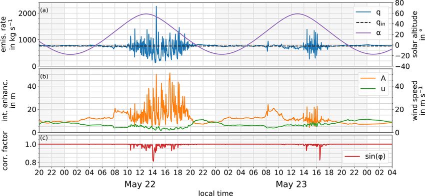
2724 S. Wolff et al.: Determination of the emission rates of CO2 point sources with airborne lidar
Figure 4. Flight track of HALO in the vicinity of the coal-fired power plant Jänschwalde. The black line on the left depicts the flight track of
HALO between 10:24 and 11:36 on 23 May 2018. The red square marks the position of the power plant Jänschwalde. The arrow shows the
mean wind direction during the observation period. The right picture shows the nine cooling towers facing southwest. There the exhaust is
released. The towers have a height of 120 m and distances of 250 and 50 m between each other.
Table 2. WRF model configuration.
Setting Reference
WRF version WRF 3.8.1 Skamarock et al. (2008)
Dynamical solvers Advanced Research WRF
Meteorological boundary conditions Operational ECMWF analysis ECMWF (2018)
Simulated time span 06:00 UTC 21 June–06:00 UTC 24 June 2018
Spin-up 6h
Number of vertical layers 56
Model top 200 hPa
Radiation Rapid Radiative Transfer Model scheme (ra_lw_physics = Iacono et al. (2008)
ra_sw_physics = 4)
Microphysics Morrison two-moment scheme (mp_physics = 10) Morrison et al. (2009)
Land surface model Unified Noah land-surface model (sf_surface_physics = 2) Tewari et al. (2004)
Surface layer physics Revised MM5 Scheme (sf_sfclay_physics = 1) Jimenez et al. (2012)
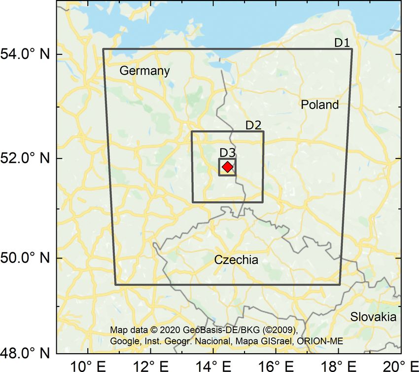
the center of the domains (see Fig. 5). The domain configu- The WRF simulation provides a data output every 2 min.
rations can be found in Table 3. As meteorological initial and One virtual plume crossing is evaluated for each output time
boundary conditions, operational ECMWF analysis data are step at a point source distance of 1.5 km. This corresponds to
used with a horizontal resolution of 9 km. our measurements (see Table 1). Since neither background
As suggested by Powers et al. (2017) we run the inner do- field nor noise is simulated, it does not matter at which dis-
main D3 as a large eddy simulation (WRF-LES). This makes tance to the point source the virtual flyover takes place. Nev-
it possible to resolve local turbulence (Moeng et al., 2007). ertheless, we try to match the virtual survey as closely as
Several studies show that WRF-LES is an adequate tool to possible to real conditions. Just as in the real measurement,
model plume trajectories, in conjunction with turbulence and the virtual crossings are arranged perpendicular to the prop-
passive tracer dispersion (Nunalee et al., 2014; Nottrott et al., agation direction of the plume (cf. Sect. 2.1). However, in a
2014). turbulent atmosphere, it is not trivial to precisely identify this
Only the plume of the power plant is simulated without direction of propagation. In this work, we consider the cen-
any CO2 background field. WRF-ARW has the option to pre- ter of mass of the emitted tracers within a radius of twice the
define a tracer variable tr(t, x, y, z) which has the properties point source distance, i.e., 3 km. A connecting line between
of a passive tracer, as used in Blaylock et al. (2017). It repre- this center of mass and the point source corresponds to the
sents a 4D field of space-time. A detailed description of the propagation direction.
calculation of simulated DAOD can be found in Appendix A. For the calculation of the virtually retrieved emission rate,
Therein Eq. (A3) is used to calculate the DAOD enhance- the mean wind speed and direction are needed (see Eq. 3).
ment corresponding to the horizontal dispersion of the tracer, To obtain these from the simulation, the following procedure
as shown in Fig. 6. is performed. First, for each data output step the horizon-
Atmos. Meas. Tech., 14, 2717–2736, 2021 https://doi.org/10.5194/amt-14-2717-2021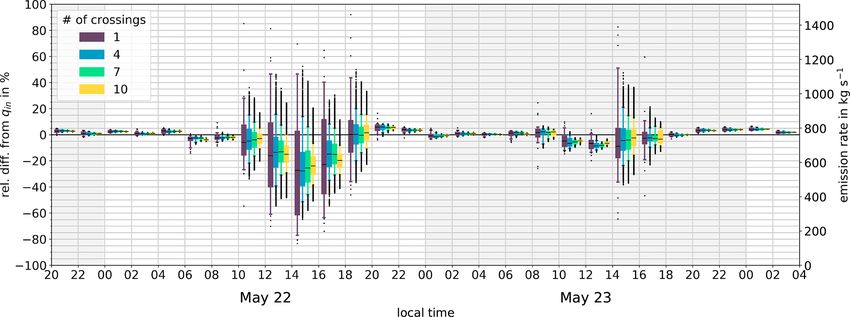
S. Wolff et al.: Determination of the emission rates of CO2 point sources with airborne lidar                                       2725

Table 3. Configuration of quadratic domains.

    Domain                          D1                                D2                                D3
    Horizontal resolution           5 km                              1 km                              0.2 km
    Computational time step         30 s                              5s                                1s
    Number of grid points           100                               150                               175
    Domain size, W–E and S–N        500 km                            150 km                            35 km
    Planetary    boundary   layer   MYNN level 2.5; Nakanishi         MYNN level 2.5; Nakanishi         LES PBL; Moeng et al. (2007)
    physics                         and Niino (2009)                  and Niino (2009)
    Eddy coefficient option         2D deformation (km_opt = 4)       2D deformation (km_opt = 4)       3D TKE (km_opt = 2)
    Turbulence and mixing option    Simple diffusion (diff_opt = 1)   Simple diffusion (diff_opt = 1)   Full diffusion (diff_opt = 2)

                                                                       Appendix A in Fig. A2. Additionally, an animated
                                                                       GIF of the simulated plume can be found under
                                                                       https://doi.org/10.5281/zenodo.4266513 (Wolff, 2020). In
                                                                       the nocturnal absence of solar irradiation, the turbulence de-
                                                                       creases, leading to narrow, homogeneous plume dispersion
                                                                       within a laminar flow. The exhaust plume follows Gaussian
                                                                       behavior, as depicted in Fig. 6 at 23:30. Contrary to this, we
                                                                       find boundary layer turbulence during daytime.
                                                                          Strong solar heating of the surface generates convective
                                                                       air masses, which in turn cause a cascade of eddies. Conse-
                                                                       quently, locally reverse and counter-gradient flow, i.e., flow
                                                                       opposite to the main wind direction, emerges. This results in
                                                                       local puffs of above-average column concentration enhance-
                                                                       ments within the exhaust plume, while eddy-generated local
                                                                       flow in the same direction as the ambient wind causes con-
                                                                       strictions of lower column concentrations in a plume (Stull,
                                                                       1988). Such plume structures deviate from Gaussian behav-
                                                                       ior, as can be seen in Fig. 6 at 17:54.
                                                                          Locally increased CO2 column concentration results in a
Figure 5. Location of three time-nested domains (black squares)
of the WRF simulation. They are centered on the power plant Jän-       high value in the integrated enhancement A in contrast to an
schwalde (red square). The domains have a side length of 500 (D1),     overflight over a constriction. Following Eq. (3) this corre-
150 (D2), and 35 km (D3) and a horizontal resolution of 5 (D1),        sponds to a high value of the emission rate q. It should also
1 (D2), and 0.2 km (D3). Vertically, 57 eta levels are introduced,     be stressed that the spatial extent of such puffs is smaller than
ranking from the ground up to a top layer pressure of 200 hPa.         that of complementary constrictions. Therefore, a skewed
                                                                       distribution of the retrieved emission rates is to be expected,
                                                                       as Fig. 7 confirms.
tal wind components at the mean height of the plume are                   On 23 May 2018, four measurement flyovers of the power
retrieved by vertical integration, weighted with tracer mass           plant Jänschwalde took approximately 1 h, as presented in
content. Second, the resulting 2D wind field is linearly inter-        Sect. 3. As spin-up we discard the first 6 h of the simulation
polated onto the virtual flight path, yielding a 1D field with         (see Table 2). That is 66 h of simulation, which leaves us with
the horizontal wind components along the flight track. Last,           a total of 1980 virtual plume flyovers. The corresponding re-
the wind components are integrated and weighted with the               sults of the emission rate, which are calculated using Eq. (3),
DAOD along the flight track, resulting in the mean wind used           are displayed as a histogram in Fig. 7 and as a time series in
for calculation.                                                       Fig. 8a.
                                                                          In Fig. 8a it can be seen how the diurnal course of so-
                                                                       lar altitude α influences the retrieved emission rates q. The
5     Simulation results                                               random occurrence of inhomogeneities in the plume propa-
                                                                       gation, caused by local turbulence, leads to large variations
WRF is able to simulate realistic plume dispersion.                    in the results of successive crossings. Turbulence lags behind
The DAOD enhancement values correspond to our mea-                     solar altitude because the surface needs time to heat up. It is
surements. Exemplary snapshots of the simulated plume
during the course of a whole day can be found in

https://doi.org/10.5194/amt-14-2717-2021                                                 Atmos. Meas. Tech., 14, 2717–2736, 2021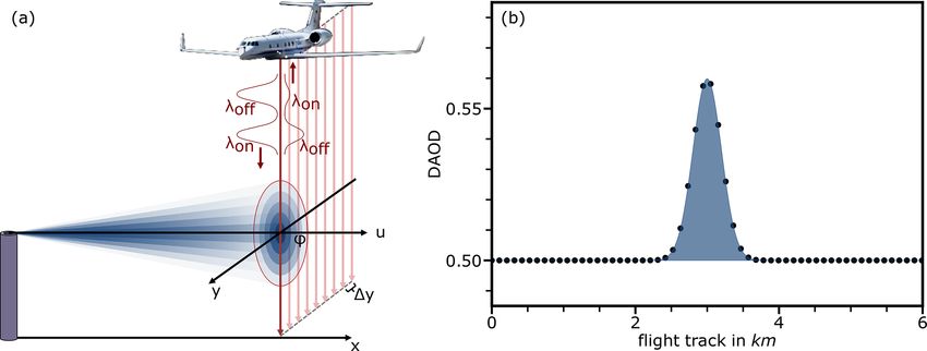
2726                            S. Wolff et al.: Determination of the emission rates of CO2 point sources with airborne lidar

Figure 6. Exemplary snapshots of simulated exhaust plumes. The flight track of the virtual plume overflight is shown as a black line. At
the top of the respective middle panels, the local time is given in Central European summer time (CEST, i.e., UTC + 2), and at the bottom
α denotes the local solar altitude. The first color bar represents the DAOD enhancement and refers to the respective middle panel, which
shows the horizontal dispersion of the plume. The second color bar represents the mass per area and refers to the top and right panels, which
show the vertical dispersion. In a corresponding measurement, DAOD enhancement values below 0.008 would not be distinguishable from
noise and are therefore displayed in blue. Values higher than 0.01 exceed the noise and can be identified as plume enhancement in a real
measurement. A 1DAOD value of 0.02 corresponds to an enhancement of 4 % with respect to a background of 0.5 (cf. Fig. 3). The color
maps follow the guidelines for a perception-based color map presented by Stauffer et al. (2015).

                                                                         cal wind speeds in the range of 5–8 m s−1 and spatial scales
                                                                         of puffs and constrictions of about 1–2 km, our range of
                                                                         time delay exceeds the residence time of coherent plume
                                                                         structures, thus preventing repeated measurements of iden-
                                                                         tical air masses. The model setup provides one measurement
                                                                         every 2 min, resulting in a vast number of permutations of
                                                                         successive virtual crossings available for merging (see Ta-
                                                                         ble A1). For each of these permutations, a mean value is cal-
                                                                         culated, which is then compared with the initiated emission
                                                                         rate qin . To evaluate the turbulence-induced inhomogeneity
                                                                         in the daily course, we compare 2 h time frames. We execute
                                                                         a total of 60 virtual overflights in such a 2 h time frame. The
                                                                         number of possible permutations increases exponentially to
                                                                         5000 if four crossings are merged and even on to 312 500 if
Figure 7. Histogram of virtually retrieved emission rates. The his-
                                                                         seven crossings are merged (see Table A1). This high num-
togram shows a slightly skewed distribution towards smaller emis-
sion rates than the input emission rate (dashed red line). It depicts    ber of permutations is based on the identical 60 single cross-
all 1980 emission rates retrieved over 66 simulated hours between        ing emission rates, which are displayed in the purple box–
12:00 UTC on 21 May and 06:00 UTC on 24 May.                             whisker plots for single crossings in Fig. 9.
                                                                            Figure 9 presents the resulting distribution of this relative
                                                                         difference to the input emission rate as a box–whisker plot.
                                                                         The spread of the respective box–whisker plot is an indicator
also apparent that the emission rate deviations vary from day            of turbulence. It is evident that with an increasing number of
to day, both in intensity and in dwell time.                             overflights merged for averaging, the spread of the relative
   The implications for the measurement results can be re-               differences decreases, while the measurement precision in-
duced by averaging over a multitude of retrieved emission                creases. A high emission rate measured by a single overflight
rates. Next, we investigate how often the exhaust plume must             scanning a puff is compensated for if the subsequent over-
be surveyed to achieve a mean emission rate with satisfactory            flight measures a lower emission rate. With a higher num-
accuracy. From experience with the Jänschwalde measure-                  ber of overflights averaged, it is more likely to measure both
ment presented in Sect. 3, as well as other point source mea-            high- and low-concentration air masses. Yet, although the
surements during the CoMet campaign which are not pre-                   precision can be improved by increasing the number of over-
sented in this work, we assume a time delay in the range                 flights, even for 10 overflights it is inferior to the precision
of 6 to 18 min between two successive crossings. With typi-

Atmos. Meas. Tech., 14, 2717–2736, 2021                                                    https://doi.org/10.5194/amt-14-2717-2021
S. Wolff et al.: Determination of the emission rates of CO2 point sources with airborne lidar 2727 Figure 8. Virtual overflight results in the course of the day. In (a) it can be seen that rising solar altitude α entails turbulence. Especially midday turbulence causes deviations in the retrieved emission rate q from the input emission rate qin . In (b) the integrated enhancement A shows equivalent behavior, while the variations in wind speed u are comparatively small. It is during the midday turbulence that the virtual flight tracks are not exactly perpendicular to the instantaneous wind direction at the plume crossing, which becomes apparent in the correction factor sin(ϕ) in (c). In the night hours, as well as the morning, the retrieved emission rates agree very well with the input emission rate qin . The wind speed u surpasses the threshold value of 2 m s−1 at all times. Figure 9. Box–whisker plot of the relative difference to the input emission rate qin within 2 h time frames. The right axis shows the associated retrieved emission rates. The width of the distribution decreases with a higher number of crossings. For all time frames it can be stated that with an increasing number of merged crossings, the width of the distribution decreases. The largest differences to qin are observed in the afternoon. Different colors represent a different number of virtual crossings merged for averaging. The inner boxes range from the first to the third quartile, thus containing 50 % of the values. The median is marked within as a black dash. The upper whisker is drawn up to the 95th percentile, while the lower whisker is drawn to the 5th percentile. Consequently, 90 % of the values are in between the two whiskers. All values outside the whiskers are outliers and plotted as dots. of nighttime measurements. Additionally, not only the pre- the true emission rate are to be expected. Here, a higher num- cision but also the accuracy is compromised during times of ber of overflights will only cause minor improvements. At strong turbulence, i.e., in the afternoon. As mentioned above, this point, it should be mentioned that the representation of the spatial extent of turbulence-induced puffs is smaller than nightly plume propagation must be critically reviewed. The the one of the complementary constrictions. Therefore, such plume height decreases so much that the propagation takes puffs are likely to be less frequent and only partially scanned place only in the lowest four model layers. The fact that a bias when measured at a low sampling frequency. Consequently, of approx. ±5 % remains at night is not surprising from this the retrieved emission rates will be biased low. This is an ef- point of view. This study should therefore be understood as a fect that occurs especially during strong turbulence. In Fig. 9 qualitative assessment. The key finding is that avoiding situa- a strongly turbulent day (22 May) is compared to a less turbu- tions of high turbulence brings an enormous improvement for lent day (23 May). Both precision and accuracy are superior both precision and accuracy. Even with a significantly higher on a less turbulent day. number of measurement overflights, a comparable improve- In contrast, the night hours show little turbulence and high ment cannot be attained. precision. Even with a single overflight, small differences to https://doi.org/10.5194/amt-14-2717-2021 Atmos. Meas. Tech., 14, 2717–2736, 2021
2728                          S. Wolff et al.: Determination of the emission rates of CO2 point sources with airborne lidar

6   Discussion                                                     ulates realistic plume dispersion. Typical DAOD values, as
                                                                   well as turbulence-induced distortions, show the same order
Regarding the lidar measurements during the CoMet cam-             of magnitude as our measurements. However, as we evaluate
paign on 23 May 2018, we find that the mean emission rate,         only four overflights in the measurement, we cannot make
derived from repeated plume overflights, is in rough agree-        any statement about the absolute accuracy of the simulation,
ment with the average emission reported by the power plant         which is also not the intention of this work. Qualitatively, the
operator for the year 2017. The cross-sectional flux method        simulation provides the following insights. During the night
is straightforward to apply. The exhaust plume generates           the plumes are weakly distorted and have a Gaussian shape
column enhancements in the differential absorption optical         because laminar flow dominates. Over the course of the day,
depth (DAOD), with a good signal-to-noise ratio, on the or-        turbulence increases, reaching its peak in the mid-afternoon
der of 10 %. The product of enhanced column concentration          and distorting the plumes to non-Gaussian shapes. Thus, with
integrated along the flight track and mean wind speed, pro-        increasing turbulence, a larger number of crossings is re-
vides the flux through the lidar cross section at the instant of   quired for averaging in order to obtain sufficient emission
the overflight. This instantaneous flux of an individual over-     rate precision. According to our simulation, nighttime mea-
flight measurement can be determined with an error rang-           surements require fewer overflights. Under such conditions,
ing between 8 %–10 %. This error is mainly driven by uncer-        even a single instantaneous cross-sectional flux measurement
tainties in the integrated enhancement, the mean differential      yields an accuracy of up to ∼ 95 %. In cases of very pro-
absorption cross section, the mean relative wind direction,        nounced turbulence (i.e., in the afternoon), even an impracti-
and the mean horizontal wind speed. On average, we find            cally high number of overflights will neither reach the preci-
that 2/10 of the flux error can be attributed to uncertainty       sion nor the accuracy of a single nighttime overflight.
in the determination of the integrated enhancement, i.e., the         At this point, we cannot derive any limits for solar alti-
integrated enhancement of the DAOD signal, which is the            tude or local times that should be avoided as the simulation
only parameter that needs to be derived from the IPDA lidar        reveals that the turbulence intensity varies from day to day
measurement. A total of 1/10 can be attributed to the un-          (see Figs. 8 and 9). Generally, we find that the most signifi-
certainties in the mean differential absorption cross section      cant turbulence occurs in the afternoon. For future campaign
of CO2 and the relative wind direction taken together. The         planning, we recommend to also perform measurements at
main source of error, however, is the mean horizontal wind         night or in the morning, which is possible with lidar.
speed with a contribution of 7/10. This highlights the need
for more accurate wind information. Future studies will ex-
amine CHARM-F measurements in the Upper Silesian Coal              7   Conclusions
Basin to determine CH4 emissions from coal mines. In this
area, ground-based Doppler wind lidars have been installed.        The present study continues the investigations by Amediek et
It is expected that nudging the simulation towards the wind        al. (2017) on the quantification of fluxes of local greenhouse
soundings will result in an improvement of the wind vector         gas emission sources using the integrated path differential
estimation, ultimately reducing the overall error in the flux      absorption (IPDA) lidar CHARM-F and the cross-sectional
determination.                                                     flux method. While the preceding study was concentrated
   It is necessary to distinguish between instantaneously          on CH4 emissions from hard coal mines, here, we exploit
measured flux and actual emission rate. In theory, an exhaust      the results from the CoMet campaign in 2018. We inves-
plume behaves Gaussian on average, and the mean emis-              tigate CO2 plume overflights of the coal-fired power plant
sion rate of the point source lies within the error range of       Jänschwalde, conducted to quantify its emission rate and to
the instantaneously measured fluxes. Contrary to this, our         assess how accurately the cross-sectional flux method can be
overflights reveal large variations between the individually       applied. Since CHARM-F measures both greenhouse gases
retrieved instantaneous fluxes which cannot be attributed to       simultaneously, our findings also apply to isolated CH4 point
measurement uncertainties. These variations do not occur be-       sources.
cause the measurement error increases, but because plume              With regard to cross-sectional flux measurements, the cur-
segments with varying CO2 content are probed. The actual           rent work suggests avoiding mid-afternoon periods of strong
measurement error is minor compared to these variations (cf.       turbulence. On the one hand, this is because the uncertainties
Table 1). As described in Sect. 5, strong solar heating causes     in the wind speed are most pronounced at these times, being
turbulence, which forces the plume to deviate from Gaussian        the major source of error in a single measurement. On the
behavior. This deviation can be restricted by averaging over       other hand, this is due to the distortions of exhaust plumes
multiple instantaneous fluxes, as the results from our mea-        in a turbulent wind field, which lead to substantial deviations
surement flights suggest.                                          from Gaussian plume dispersion. Under strong turbulence,
   To analyze this effect in more detail, we employ the at-        the cross-sectional flux method cannot provide an accurate
mospheric transport model WRF in a high-resolution large           measurement of the emission rate, not even in the average of
eddy simulation (LES) setup. We find that the model sim-           a vast number of overflights. Therefore, measurement flights

Atmos. Meas. Tech., 14, 2717–2736, 2021                                             https://doi.org/10.5194/amt-14-2717-2021
S. Wolff et al.: Determination of the emission rates of CO2 point sources with airborne lidar 2729 performed during nighttime are beneficial. In this respect, 8 Outlook intrinsic independence from solar irradiation is a clear ad- vantage of active remote sensing over passive approaches. Apart from the CHARM-F measurements, the CoMet cam- Whenever sunlight is needed to perform the measurement, paign also saw the deployment of other airborne instruments less turbulent conditions, for example in the morning after to measure atmospheric CH4 and CO2 , supported by a vari- sunrise or winter, should be preferred. Further, it should be ety of ground-based, in situ, and remote sensing instruments. pointed out that, with a lidar, cross-sectional plume measure- They were predominantly based in the vicinity of one of the ments can also be performed over water bodies whose detri- major hot-spot regions of CH4 emissions in Europe, the Up- mental reflective properties often impede the use of passive per Silesian Coal Basin (USCB). Investigations of local and remote sensing (Gerilowski et al., 2015; Krautwurst et al., regional CH4 emissions from this region are, in view of the 2021; Larsen and Stamnes, 2006). Therefore, plumes from preparation for the upcoming MERLIN mission, a particular offshore installations can also be addressed with this ap- field of interest. The possibility to synergistically use active proach. remote sensing (lidar), passive spectrometry, and in situ mea- Independent of the location of the point source, there are surements supported by modeling activities allows for unique restrictions regarding the adequate distance of a plume over- cross comparisons, which are beyond the scope of the present flight to the point source. We report that at a point source paper. Such cross comparisons will be the subject of subse- distance of more than 4.6 km no enhancement is visible and quent investigations, as well as other HALO measurement therefore no plume detection can be performed. In addition flights, as it flew along latitudinal trajectories, performed re- to that, we find that the uncertainty of the mean differential gional survey flights (e.g., over Mount Etna), and also probed absorption cross section increases with a larger vertical ex- the local plume of not only Jänschwalde but also Bełchatów tension of the plume which correlates with distance. At a in Poland, which is considered Europe’s largest coal-fired point source distance of 1.5 km, this uncertainty is negligi- power plant in terms of CO2 emission. The measured data ble. Concerning the detectability of the plume, we can locate can make an important contribution to the validation of ex- distinct enhancements at a distance of 1.5 km. Nevertheless, isting satellite missions (e.g., Sentinel-5P, GOSAT). Further the closer to the point source the overflight takes place, the aircraft campaigns (e.g., CoMet-2.0) are foreseen which will more constrained the plume and consequently the more pro- provide additional opportunities for methodical refinements, nounced the column enhancement is. It must be considered, including advancements in model-measurement synergies. however, that the horizontal extension is also smaller, and thus fewer data points lie within the plume. In the case of CHARM-F, this can be compensated for by a higher repeti- tion rate. https://doi.org/10.5194/amt-14-2717-2021 Atmos. Meas. Tech., 14, 2717–2736, 2021
You can also read