TOWARDS A GLOBAL UNDERSTANDING OF VEGETATION-CLIMATE DYNAMICS AT MULTIPLE TIMESCALES - MPG.PURE
←
→
Page content transcription
If your browser does not render page correctly, please read the page content below
Biogeosciences, 17, 945–962, 2020
https://doi.org/10.5194/bg-17-945-2020
© Author(s) 2020. This work is distributed under
the Creative Commons Attribution 4.0 License.

Towards a global understanding of vegetation–climate dynamics
at multiple timescales
Nora Linscheid1,2, , Lina M. Estupinan-Suarez1,3, , Alexander Brenning3,4 , Nuno Carvalhais1,5 , Felix Cremer3,6 ,
Fabian Gans1 , Anja Rammig2 , Markus Reichstein1,4,7 , Carlos A. Sierra1 , and Miguel D. Mahecha1,4,7
1 Max   Planck Institute for Biogeochemistry, Hans-Knöll-Str. 10, 07745 Jena, Germany
2 TUM    School of Life Sciences Weihenstephan, Technical University of Munich, Hans-Carl-von-Carlowitz-Platz 2,
85354 Freising, Germany
3 Department of Geography, Friedrich Schiller University Jena, Löbdergraben 32, 07743 Jena, Germany
4 Michael Stifel Center Jena for Data-Driven and Simulation Science, Ernst-Abbe-Platz 2, 07743 Jena, Germany
5 Departamento de Ciencias e Engenharia do Ambiente, DCEA, Faculdade de Ciencias e Tecnologia,

FCT Universidade Nova de Lisboa, Caparica, Portugal
6 Institute for Data Science, German Aerospace Center (DLR), 07745 Jena, Germany
7 German Centre for Integrative Biodiversity Research (iDiv) Halle-Jena-Leipzig, Deutscher Platz 5e,

04103 Leipzig, Germany
 These authors contributed equally to this work.

Correspondence: Nora Linscheid (nlinsch@bgc-jena.mpg.de) and Lina M. Estupinan-Suarez (lestup@bgc-jena.mpg.de)

Received: 15 August 2019 – Discussion started: 17 September 2019
Revised: 23 December 2019 – Accepted: 14 January 2020 – Published: 24 February 2020

Abstract. Climate variables carry signatures of variability at         especially in the tropics. Finally, we find that correlations
multiple timescales. How these modes of variability are re-            between variables can differ and even invert signs across
flected in the state of the terrestrial biosphere is still not quan-   timescales. For southern Africa for example, correlation be-
tified or discussed at the global scale. Here, we set out to gain      tween NDVI and Tair is positive for the seasonal signal but
a global understanding of the relevance of different modes of          negative for short-term and longer-term oscillations, indicat-
variability in vegetation greenness and its covariability with         ing that both short- and long-term temperature anomalies can
climate. We used > 30 years of remote sensing records of the           induce stress on vegetation dynamics. Such contrasting cor-
normalized difference vegetation index (NDVI) to character-            relations between timescales exist for 15 % of vegetated ar-
ize biosphere variability across timescales from submonthly            eas for NDVI with Tair and 27 % with Prec, indicating global
oscillations to decadal trends using discrete Fourier decom-           relevance of scale-specific climate sensitivities.
position. Climate data of air temperature (Tair ) and precipita-          Our analysis provides a detailed picture of vegetation–
tion (Prec) were used to characterize atmosphere–biosphere             climate covariability globally, characterizing ecosystems by
covariability at each timescale.                                       their intrinsic modes of temporal variability. We find that
    Our results show that short-term (intra-annual) and longer-        (i) correlations of NDVI with climate can differ between
term (interannual and longer) modes of variability make re-            scales, (ii) nondominant subsignals in climate variables may
gionally highly important contributions to NDVI variability:           dominate the biospheric response, and (iii) possible links
short-term oscillations focus in the tropics where they shape          may exist between short-term and longer-term scales. These
27 % of NDVI variability. Longer-term oscillations shape               heterogeneous ecosystem responses on different timescales
9 % of NDVI variability, dominantly in semiarid shrublands.            may depend on climate zone and vegetation type, and they
Assessing dominant timescales of vegetation–climate covari-            are to date not well understood and do not always correspond
ation, a natural surface classification emerges which cap-             to transitions in dominant vegetation types. These scale de-
tures patterns not represented by conventional classifications,

Published by Copernicus Publications on behalf of the European Geosciences Union.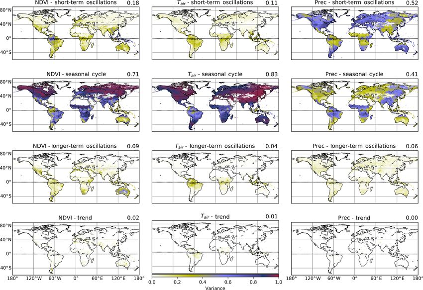
946                                                                N. Linscheid et al.: Multiscale vegetation–climate dynamics

pendencies can be a benchmark for vegetation model evalu-            and long-term processes can be obscured by the dominant in-
ation and for comparing remote sensing products.                     fluence of the annual cycle (Braswell et al., 2005; Mahecha
                                                                     et al., 2010c). In order to study relevant ecosystem–climate
                                                                     interactions across temporal scales, information contained
                                                                     for each timescale thus first needs to be extracted from this
1   Introduction                                                     integrated signal. Time series decomposition allows us to ex-
                                                                     tract different frequencies such as annual, intra-annual, and
Ecosystems and climate interact on multiple spatial and tem-         interannual oscillations from vegetation and climate time se-
poral scales. For example, the main driver of photosynthe-           ries. Such approaches have proven useful, e.g., to character-
sis during the daily cycle typically is light availability, as-      ize at what scales vegetation responses are dampened or am-
suming no other resource limitation. At annual timescales,           plified in comparison with their climate forcing (Stoy et al.,
temperature can limit growth and development during cer-             2009), how ecosystem variability is confined by hydrome-
tain phases of the year, particularly in the extratropics. While     teorological variability (Pappas et al., 2017), what scales of
climate variability is traditionally very well characterized         variability need to be considered to relate forcing variables
across timescales (e.g., Viles, 2003; Cao et al., 2012; Bala         and vegetation state comprehensively (Katul et al., 2001;
et al., 2010; Hannachi et al., 2017), it is less well known          Braswell et al., 2005), or to remove confounding effects from
how the biosphere responds to variations in climate on differ-       processes acting on longer timescales than the process in
ent scales. Understanding the implications of such timescale         question (Mahecha et al., 2010b). However, to date most
dependencies of climate–vegetation interactions is challeng-         studies employing time series decomposition to study veg-
ing due to the variety of interwoven processes. These de-            etation dynamics have focused on disentangling timescales
pendencies range from short-term climate extremes and bi-            from minutes to a few years based on flux data (Stoy et al.,
otic stress (e.g., insect outbreaks) to seasonal dynamics in         2009; Katul et al., 2001; Mahecha et al., 2007, 2010c). Stud-
climate-driven phenology and long-term dynamics that can             ies investigating long-term vegetation records by time se-
again either reflect intrinsic ecosystem dynamics (e.g., veg-        ries decomposition do exist but focus only on a specific re-
etation successional dynamics) or climate-change- or land-           gion (Martínez and Gilabert, 2009; Canisius et al., 2007;
use-induced process alterations. Investigating vegetation–           Hawinkel et al., 2015) or do not provide cointerpretation with
climate dynamics globally across multiple timescales re-             climate signals (Pan et al., 2018). Earth observation time se-
quires long-term observation on relevant vegetation dynam-           ries of vegetation and climate covering more than 30 years
ics and climate variables in combination with a method to            now allow us to characterize the timescale-resolved variabil-
separate ecosystem variability at different timescales.              ity in the biosphere and its relation to climate globally across
   The assessment of ecosystem variability, e.g., in responses       several decades. Additionally, the global coverage of these
to climate at the global scale, has only become feasible in          records allows one to attain a broader understanding in cli-
the last decades. Long-term Earth observations (EOs) are             mate space and across vegetation types, which to date is
now allowing us to assess ecosystem states consistently over         equally lacking.
more than 30 years. Vegetation indices such as the normal-              In this study, we set out to gain a global understand-
ized difference vegetation index (NDVI) have often been in-          ing of the relevance of the different modes of variabil-
terpreted as proxies for vegetation activity (Zeng et al., 2013;     ity in vegetation greenness and its covariability with cli-
De Keersmaecker et al., 2015; Hawinkel et al., 2015; Kogan           mate at timescales from submonthly oscillations to long-
and Guo, 2017; Pan et al., 2018), despite well-known limi-           term trends. These timescale-specific vegetation–climate co-
tations of only reflecting vegetation greenness. While novel         oscillations are expected to serve as a reference benchmark
EOs may be more closely related to actual rates of photosyn-         for comparing remote sensing products and terrestrial bio-
thesis (Sun-induced fluorescence, SIF; Guanter et al., 2007),        sphere models. Specifically, we aim to (i) characterize vari-
NDVI from the Advanced Very High Resolution Radiome-                 ability of biosphere and climate time series explicitly on
ter (AVHRR) has the advantage of offering the longest up-            multiple timescales; (ii) understand spatial patterns of this
dated records of vegetation remote sensing data every 15 d           scale-resolved variability and covariability globally; (iii) as-
(d stands for day). In tandem with climate time series from          sess whether characteristic timescale-specific dynamics in
the same period, this record provides a solid basis to globally      the biosphere and climate relate to established climate classi-
assess biosphere–atmosphere interactions across timescales           fications or land cover; and (vi) assess differences in correla-
ranging from weeks to decades.                                       tions of biosphere with climate on short-term, seasonal, and
   Temporal biosphere dynamics carry the imprint of dif-             longer-term timescales.
ferent drivers across timescales, yet EOs can only record
one integrated signal over time. This signal reflects a mix-
ture of processes acting on different scales, which cannot
be observed independently (Mahecha et al., 2007; Defriez
and Reuman, 2017; Pan et al., 2018). Therefore, short-term

Biogeosciences, 17, 945–962, 2020                                                          www.biogeosciences.net/17/945/2020/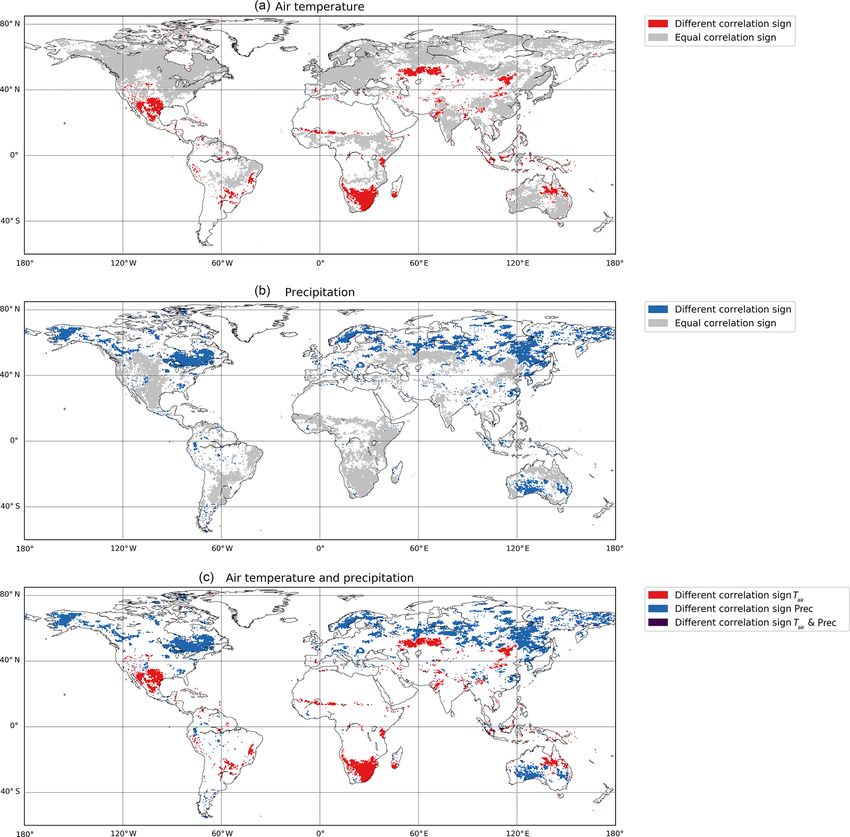
N. Linscheid et al.: Multiscale vegetation–climate dynamics                                                                  947

2     Methods                                                    sonal, and longer-term oscillations: the seasonal signal was
                                                                 reconstructed from the Fourier spectrum at periods of 0.9–
The code to produce all primary figures is made available        1.1 years, plus semiannual and 4-monthly harmonics (i.e.,
as supplementary notebook (https://doi.org/10.5281/zenodo.       0.5- and 0.33-year periods). The short-term signal was recon-
3611262, Linscheid et al., 2019).                                structed from the Fourier spectrum of all periods < 0.9 year,
                                                                 except the two seasonal harmonics, representing interannual
2.1    Data                                                      oscillations that are not directly linked to periods of sea-
                                                                 sonality. The longer-term signal was reconstructed from all
A global gridded dataset of AVHRR NDVI was retrieved
                                                                 remaining periods > 1.1 year, representing interannual and
from the Global Inventory Monitoring and Modeling Sys-
                                                                 longer timescales. The subsignal binning was centered on the
tem (GIMMS, Pinzon and Tucker, 2014) at 15 d tempo-
                                                                 definition of the seasonal/annual bin similarly to Mahecha
ral and 0.083◦ spatial resolutions (GIMMS NDVI v3.1).
                                                                 et al. (2010a) and Fürst (2009). The bin ranges were slightly
Original data were aggregated to 0.5◦ by taking the mean
                                                                 adapted due to the FFT approach, which yields signals of
of the corresponding 0.083◦ pixels. Corresponding records
                                                                 different frequencies compared to the approach chosen by
of air temperature (Tair ) from the European Centre for
                                                                 Mahecha et al. (2010a). To identify emerging features occur-
Medium-Range Weather Forecasts (ERA-Interim v4, Dee
                                                                 ring at different latitudinal bands, mean values weighted by
et al., 2011) and precipitation (Prec) from the Multi-Source
                                                                 pixel area were calculated in the tropics (23.5◦ N to 23.5◦ S),
Weighted-Ensemble Precipitation (MSWEP, Beck et al.,
                                                                 extratropics (above 23.5◦ N and below 23.5◦ S), and globally.
2019) were aggregated to match temporal resolution by sum-
mation (Prec) or averaging (Tair ). Spatial resolution of Tair   2.4   Variance per timescale and co-oscillation regimes
was preserved (0.5◦ ), while MSWEP values were averaged
for spatial resampling (0.083 to 0.5◦ ). Spatial and temporal    For each timescale-specific signal, we calculated the propor-
resolution were fixed based on the coarsest resolution among     tion of variance of the original signal explained for each vari-
the input datasets to ensure conservative results. The time      able per grid cell. Each pixel of the global land surface was
period considered was from 1 January 1982 to 31 Decem-           then classified into oscillation regimes depending on which
ber 2015.                                                        scale explained the largest amount of variance in each vari-
                                                                 able (abbreviations: S – short term, A – seasonal, L – longer
2.2    Preprocessing                                             term, T – trend). For example, if the variance was dominated
                                                                 by the seasonal subsignal in NDVI and Tair , and by the short-
Gaps in NDVI time series were filled with values from the        term scale in Prec, this pixel would be classified as AAS (in
mean seasonal cycle computed separately for each grid cell.      the order of NDVI, Tair , and Prec). Theoretically, the super-
Missing values were mostly present at high northern latitudes    imposition yields 64 (43 ) possible combinations, of which
(Fig. S1 in the Supplement). Each time series (for each pixel)   only 26 occurred. For simplicity, our analysis was focused
was normalized to zero mean and unit variance prior to per-      on the 11 most abundant oscillation regimes (99.7 % of pix-
forming fast Fourier transformation (FFT). For further anal-     els).
ysis, the gap-filled data were discarded. Normalization, gap-       In order to complement static/traditional classifications,
filling, and FFT were performed in the Earth System Data         we compared our oscillation regimes with the Global Land
Lab (https://www.earthsystemdatalab.net/, last access: 1 Au-     Cover map project coordinated by the Joint Research Cen-
gust 2019, Mahecha et al., 2019), using the implementation       ter (GLC2000, Bartholomé and Belward, 2005) and climate
based on the programming language Julia. Analyses were           zones from the updated Köppen–Geiger global classification
performed on a latitude–longitude grid due to software and       (Kottek et al., 2006, see Fig. S1). Only those pixels that
data considerations. In all spatial analyses on the latitude–    contained data from all three data streams (Köppen–Geiger
longitude grid, the difference in size of grid cells between     classes A–D, GLC2000, and our oscillation regimes) were
high latitudes and the Equator was accounted for through         considered in this analysis. Nonvegetated and nonnatural ar-
weighting values by grid cell size. Similarly, in all analyses   eas as defined by GLC2000 were disregarded for this analy-
that involved sampling of data points, the sampling frequency    sis and onward (Table S1 in the Supplement). The final land
was weighted by grid cell size.                                  surface assessed was 75 871 486 km2 , corresponding to 70 %
                                                                 of the vegetated GLC2000 area (Fig. S1). For the same area,
2.3    Time series decomposition
                                                                 we calculated the V measure (V ), a spatial association in-
All pixel time series were first detrended using a linear        dex based on homogeneity and complementarity criteria pro-
model. We then used discrete FFT to decompose the de-            posed specifically for thematic map comparison (Nowosad
trended time series into underlying harmonic functions at dif-   and Stepinski, 2018). The index ranges from 0 to 1, with 1
ferent frequencies (Brockwell and Davis, 2006). The result-      being a perfect association, and was used to provide an over-
ing Fourier spectra (Fig. S2) were reconstructed by inverse      all comparison between the co-oscillation regime map with
FFT into binned scale-specific subsignals for short-term, sea-   Köppen–Geiger and GLC2000 maps.

www.biogeosciences.net/17/945/2020/                                                        Biogeosciences, 17, 945–962, 2020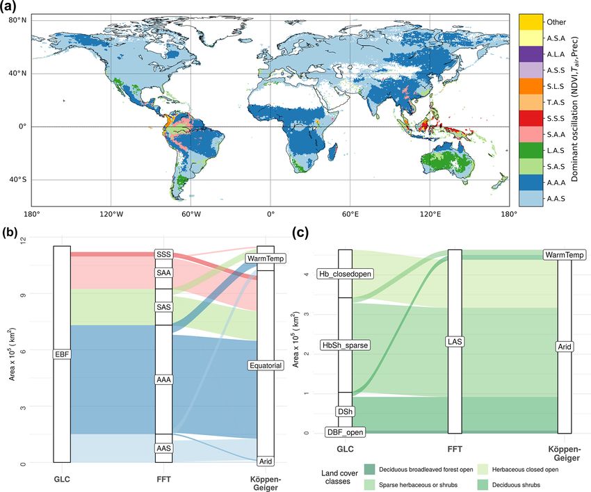
948                                                                 N. Linscheid et al.: Multiscale vegetation–climate dynamics

   To assess the influence of gap-filling performed in the orig-      seasonal and longer-term oscillations to detect areas where
inal GIMMS NDVI data due to influence of cloud cover or               the correlation was inverted between scales.
snow, we excluded time points that were retrieved by splines
or mean seasonal cycle due to the lack of direct observation          2.6   Assessment of land cover change on time series
in NDVI (Pinzon and Tucker, 2014) at five different qual-                   decomposition
ity flag thresholds in our classification of oscillation regimes.
Quality flags were aggregated from 0.083 to 0.5◦ by calculat-         We assessed whether land cover change over the 30-year
ing the fraction of direct observations per 0.5◦ pixel at each        time period influenced our results by extracting pixels with
time step. Subsequently, the dominant classification was re-          substantial land cover change as determined by Song et al.
peated, excluding time steps with less than 30 %, 50 %, 70 %,         (2018). While linear trends were removed from the time se-
90 %, and 95 % direct observations for each grid cell. Fur-           ries before decomposition, changes in amplitude or piece-
thermore, we repeated the time series decomposition method            wise linear and nonlinear trends may have an impact on our
for NDVI and the enhanced vegetation index (EVI) from the             analyses. First, we aggregated original 0.05◦ data to match
Moderate Resolution Imaging Spectroradiometer (MODIS).                our 0.5◦ spatial resolution by averaging. We then determined
The vegetation indices product MOD13C1.006 is provided                0.5◦ pixels with > 25 % gain or loss of trees, short vege-
by NASA EOSDIS LP DAAC at 0.05◦ . Data were aggregated                tation, or bare ground and assessed whether the observed
spatially by averaging valid pixels to 0.5◦ for the overlapping       changes in land cover (Song et al., 2018) were reflected in
period with GIMMS NDVI (2001–2015). A comparison of                   the NDVI time series to a degree that substantially affected
the dominant oscillation regimes between products was car-            the classification of dominant oscillation regimes.
ried out at a pixel basis.
                                                                      2.7   Comparison of Fourier transform with empirical
                                                                            mode decomposition
2.5   Correlations between variables at each timescale
                                                                      While the FFT approach is the most classical time series
We correlated timescale-specific subsignals of NDVI, Tair ,           decomposition technique, there are more data-adaptive al-
and Prec using Pearson’s correlation coefficient, Spearman            ternatives available (Huang et al., 1998; Ghil, 2002; Paluš
correlation, and partial correlation. For this analysis, all time     and Novotná, 2008). In order to understand whether differ-
points with NDVI < 0.2 were masked in order to consider               ent methods would lead to different insight, we compared the
only data points corresponding to active vegetation (Fig. S1).        employed FFT approach with the more data-adaptive empir-
NDVI was lagged one time step (15 d) behind Prec in order             ical mode decomposition (EMD). EMD repeatedly extracts
to allow for the response time of vegetation to changes in            subsignals (intrinsic mode functions, IMFs) from the time
water availability. Due to the 15 d temporal resolution of the        series by interpolating a spline between local minima and
data, a response time of up to 15 d is intrinsically included         maxima until the residuals converge to approximately con-
in our analyses. Each time lag is therefore an additional 15 d,       stant values (Huang et al., 1998). We used an ensemble-based
and shorter responses cannot be assessed. We compared six             modification of the EMD algorithm, the complete ensemble
different lags (from 15 to 90 d, Fig. S3). When correlating           empirical mode decomposition with adaptive noise (CEEM-
NDVI and precipitation instantaneously, we found almost ex-           DAN, Colominas et al., 2014; Torres et al., 2011), and a
clusively negative correlations for the short-term scale. A lag       frequency-binning approach to obtain frequency bands com-
of one time step was sufficient to arrive at expected posi-           parable to the ones chosen for FFT. In contrast to the regular
tive correlations between NDVI and precipitation, while in-           EMD, CEEMDAN employs an ensemble approach in which
creasing the lag time did not substantially improve or alter          noise is added to the data before decomposition and ensem-
the results. We thus chose to globally use a lag of one time          ble averages for each IMF are returned, so that a more ro-
step (representing a 15–30 d response time) between precip-           bust end result is obtained (Colominas et al., 2014; Torres
itation and NDVI across all scales. Globally, temperature             et al., 2011). Briefly, in CEEMDAN each IMF is computed
appeared to be most strongly correlated to NDVI instanta-             as the mean of an ensemble of IMFs retrieved from noisy
neously (not lagged); thus, no time lag was introduced be-            data copies. This IMF is subtracted from the original signal,
tween air temperature and NDVI. Recent studies assessing              and the residual signal is used as input for retrieving the next
time lags and memory effects between vegetation and cli-              IMF (Colominas et al., 2014; Torres et al., 2011). As such,
mate also indicate that time lags of around 1 month gener-            CEEMDAN is less prone to mode mixing than EMD while
ally carry most of the explanatory power for predicting veg-          still fulfilling the completeness property of EMD (i.e., the
etation dynamics (Krich et al., 2019; Kraft et al., 2019; Pa-         sum of all IMFs equals the original signal). As IMFs result-
pagiannopoulou et al., 2017). Correlations of NDVI–Tair and           ing from EMD do not have a fixed frequency assigned, we
NDVI–Prec were binned into five quantiles and presented in            then associated each IMF with a timescale by measuring the
a bivariate color map (Teuling et al., 2011). In addition, we         distance between all local maxima and minima as a proxy for
compared differences in the sign of the correlation between           the dominating wavelength of the signal. Distances between

Biogeosciences, 17, 945–962, 2020                                                           www.biogeosciences.net/17/945/2020/
N. Linscheid et al.: Multiscale vegetation–climate dynamics 949
each two maxima or minima were classified as short-term, we find that seasonal NDVI regimes co-occur predominantly
seasonal, or longer-term depending on their length. The IMF with seasonal Tair , as well as seasonal or short-term Prec
was then categorized by the majority distance category and regimes (blue regions). Dominant seasonal cycles of NDVI
added into the respective timescale bin. For example, if an and Tair , as well as fast oscillation regimes in Prec, are ex-
IMF contained 25 seasonal cycles and 5 short-term cycles, it pected over large parts of the globe, which is reflected by
was classified as seasonal and added to the seasonal signal the large extent of the AAS and AAA classes in this anal-
bin. IMFs in each bin were combined by summation. ysis. Beyond this expected solar-cycle-induced behavior, a
number of differentiated oscillation classes stand out: short-
term NDVI oscillations occur mainly in the South American
3 Results and Asian tropics, in a multitude of combinations with pre-
dominantly seasonal or short-term Tair and Prec (light-green,
3.1 Time series variance across timescales
red, and light-red regions). Longer-term oscillation regimes
Assessing the contribution of each timescale subsignal to the of NDVI co-occur with seasonal Tair and short-term Prec
signal variance at each grid cell, we find that for NDVI most regimes (dark green regions) around southwestern Africa,
of the temporal variability is expectedly captured by the sea- southeastern South America, and Australia. Interestingly, the
sonal cycle (71 % of the global variance), especially above dominant scales in climatic variables are not always associ-
the Tropic of Cancer (23.5◦ N) (Fig. 1, Table S2). Short- ated with similar dominant regimes in NDVI dynamics, sug-
term oscillations contribute dominantly in parts of tropi- gesting complex or additional driving mechanisms in these
cal America and Southeast Asia, while longer-term compo- heterogeneous regions. In fact, even in areas where tempera-
nents are mainly observed in Australia, South Africa, parts ture or precipitation has a seasonal cycle, NDVI can be dom-
of Argentina, and northern Mexico. Specifically, short-term inated by short-term or longer-term oscillations: more than
and longer-term signals together contribute 27 % of the to- 90 % of the area with short-term NDVI regimes exhibits pre-
tal NDVI variance globally and 38 % in the equatorial region dominantly seasonal Tair , of which 36 % also shows predom-
(23.5◦ N to 23.5◦ S). inantly seasonal Prec (SAA) and 55 % predominantly short-
Similarly, Tair is strongly dominated by seasonal oscilla- term Prec (SAS, Table S3). All areas where NDVI is predom-
tions in the extratropics above/below 23.5◦ N/S (94 % and inantly longer term are classified as seasonal Tair and short-
90 %, respectively, Table S2) as would be expected. Even term Prec regimes (LAS, Table S3).
in the tropics, short-term and longer-term components con- To account for the influence of clouds and snow cover
tribute only 30 % of the variance (and 11 % and 4 % of global in the GIMMS NDVI record, especially in the tropics and
variance, respectively, Table S2). In contrast, short-term os- northern regions, we excluded time points where pixels con-
cillations dominate global precipitation variance before the tained a high proportion of gap-filled values. We found that
seasonal cycle (52 % and 41 % of global variance each, Ta- overall less than 1.5 % of pixels changed their dominant
ble S2). An east–west gradient of precipitation over Eurasia oscillation class when only pixels with more than 0.7 di-
stands out, changing from predominantly short-term to pre- rect observation fraction were considered. Even when the
dominantly seasonal signal variance. In the tropics, a sim- highest-quality threshold was applied (0.95 direct observa-
ilar contribution from both oscillations is found (42 % and tion fraction), only 2.6 % of pixels changed dominant oscil-
41 %, respectively, Table S2). Linear trends removed before lation class (Fig. S5). Short-term pixels were the most af-
FFT decomposition had a minor influence on overall vari- fected by changes in dominant oscillation (12.9 % and 20.8 %
ance (Fig. 1). In summary, short-term and longer-term signals for 0.7 and 0.95 direct observation thresholds respectively),
show substantial, regionally focused contributions to signal while seasonal pixels showed the highest fraction of gap-
variance. These regions differ between variables, suggesting filling overall (Fig. S5). As a further validation, we found
complex patterns of temporal interaction. very similar results when repeating the time series decom-
position and the dominant oscillation regime classification
3.2 Classification of co-oscillations regimes based on EVI and NDVI from MODIS (Didan et al., 2019;
Huete, 1997; Huete et al., 2002) for the years 2001–2015
Given the contrasting, spatially heterogeneous patterns ob- (Fig. S6).
served in different variables in Fig. 1, we investigated how We investigated to what extent our classification into os-
scale-specific oscillations of biosphere and climate co-occur cillation regimes shows patterns of temporal vegetation–
globally. We combined the dominant scale of variability for climate relations that are not represented by conventional
each variable in each grid cell (Fig. S4) and found that 84.5 % static classifications of the land surface. To determine over-
of the assessed area is dominated by seasonal oscillations of lap and differences between the classification of tempo-
NDVI, 9 % by short-term oscillations in NDVI, and 6.5 % ral vegetation–climate co-oscillations with static classifica-
by longer-term oscillations in NDVI (0.03 % captured by the tions of land cover (GLC2000) and Köppen–Geiger climate
trend). Combining the maps for all three variables into a classes, we assessed their spatial association by the V mea-
map of codominant oscillation regimes (Fig. 2, Table S3), sure (Nowosad and Stepinski, 2018). The V measures of co-
www.biogeosciences.net/17/945/2020/ Biogeosciences, 17, 945–962, 2020950 N. Linscheid et al.: Multiscale vegetation–climate dynamics Figure 1. Global distribution of timescale-specific variance (relative spectral powers) of the normalized difference vegetation index (NDVI), air temperature (Tair ), and precipitation (Prec). Normalized time series of NDVI, Tair , and Prec (columns) were decomposed by fast Fourier transformation and reconstructed into short-term (intra-annual), seasonal (annual), and longer-term (interannual) components (rows). The relative contribution of each scale-specific signal to overall variance was determined at each grid cell. Globally, most of the variance of NDVI and Tair is contained in the seasonal component (red colors), while Prec shows a high contribution of variance from the short-term component. The semiannual cycle is included in the seasonal band. Upper-right-corner values show the percentage of overall variance explained by each timescale. oscillation regimes with Köppen–Geiger and GLC2000 were oscillation (Fig. 2b). In contrast, more than 95 % of decidu- V = 0.17 and V = 0.11, respectively, indicating weak asso- ous and evergreen needleleaf forests (DNF and ENF) and de- ciation with both static classifications. Hence, our classifica- ciduous broadleaf forests (DBF) are dominated by seasonal tion contains information largely complementary to the com- NDVI regimes (Table S3). We further find a strong associa- pared climate and land cover classifications. Yet we observed tion of longer-term NDVI regimes with shrubs (21 % of the a slightly stronger association with Köppen–Geiger than with area dominated by longer-term NDVI), herbaceous (26 %), GLC2000, also when comparing homogeneity and comple- and sparse shrubs/herbaceous (49 %) land cover types in arid mentarity (Table S4). Comparing the three classifications regions (Fig. 2c, overall 93 % of the LAS area coincides among each other, we find that dominant temporal patterns in with Köppen–Geiger class B). Thus, differences within and NDVI can be linked to certain land cover types such as shrubs among land cover and climate types exist when assessing and broadleaf forest: Sankey diagrams (Fig. 2b and c) dis- temporal co-oscillations of vegetation and climate. play which proportion of land surface is commonly classified across different class combinations in the three data layers 3.3 Assessment of land cover change on time series of the co-oscillation regime, GLC2000, and Köppen–Geiger decomposition for evergreen broadleaf forest (EBF, Fig. 2b) and areas domi- nated by longer-term NDVI (Fig. 2c). We find that EBF is the In the above analyses we did not aim to explicitly detect the most diverse among land cover classes in terms of our tempo- effect of land cover or land use change (LCLUC), but never- ral classification, with 35 % dominated by short-term NDVI theless LCLUC could have an influence on our NDVI classi- Biogeosciences, 17, 945–962, 2020 www.biogeosciences.net/17/945/2020/
N. Linscheid et al.: Multiscale vegetation–climate dynamics                                                                             951

Figure 2. Classification of land surface by dominant scale of variability in NDVI and climate, and its relation to land cover and mean
climate. (a) Dominant scale of variability was determined for NDVI, Tair , and Prec separately for each grid cell and summarized as unique
combinations between variables (S – short term, A – seasonal, L – longer term, T – trend, listed in the order of NDVI, Tair , and Prec). Only
the 11 most common classes are shown. The semiannual cycle is included in the seasonal band. (b, c) Sankey diagrams (river plots) showing
associations of pixels for (b) evergreen broadleaf forest (EBF) and (c) regions of dominant long-term oscillations in NDVI (LAS class) to
oscillation regime (FFT), land cover class (GLC2000), and Köppen–Geiger (KG) climate class. The width of the ribbons is proportional
to the area that is commonly classified into the corresponding GLC2000, KG, or oscillation classes. DBF: deciduous broadleaf forest;
Hb_closedopen: herbaceous closed open land cover; DSh: deciduous shrublands; HbSh_sparse: sparse herbaceous and shrub vegetation;
Equatorial: KG class A; Arid: KG class B; WarmTemp: KG class C; NDVI: normalized difference vegetation index; Tair : air temperature;
Prec: precipitation.

fication (Fig. 2). We assessed whether changes in vegetation             Fensholt et al., 2015): at 0.5◦ resolution, most pixels rep-
cover over the 30-year period severely affected our classifi-            resent mixed signals which obscure most of the details that
cation by inspecting pixels with > 25 % change in the frac-              would allow for detecting land cover changes. In those pix-
tion of trees, short vegetation, or bare ground according to             els where we did see a clear progression in NDVI over time,
Song et al. (2018). Notably, very few of such pixels showed              the method did adequately capture this progression, e.g., by
marked signs of land cover change reflected in NDVI time                 correctly reflecting an increasing amplitude of the seasonal
series at all, which is likely due to the coarse spatial reso-           cycle and/or shifting baseline (Fig. S7). However, the ma-
lution of the data used in this study as compared to previ-              jority of such pixels with pronounced positive or negative
ous studies focused on detecting LCLUC (Song et al., 2018;               NDVI progression were located in agricultural areas or ar-

www.biogeosciences.net/17/945/2020/                                                                  Biogeosciences, 17, 945–962, 2020
952 N. Linscheid et al.: Multiscale vegetation–climate dynamics
eas of urbanization, which had a priori been excluded from ferentiating effect for correlation patterns, and different cli-
downstream analyses. Overall, the change in vegetation over mate classes occupy distinct patterns in this correlation space
time did not have a widespread influence on the classification across scales (Fig. S12). Different land cover types generally
of dominant scale and oscillation regimes at the given spatial show similar correlations within one climate zone, but ex-
resolution. ceptions exist (Fig. S13). Most prominently, EBF shows the
most heterogeneous, spatially varying correlations on a sea-
3.4 Correlations of NDVI with climate on multiple sonal scale. All land cover types show a confined correlation
scales pattern of mainly Tair +/Prec− or Tair −/Prec+ at the longer-
term scale (Fig. 3c), which is further differentiated by climate
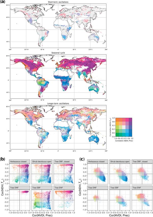
To inspect relationships of vegetation with climate at multi- zone (Fig. S14).
ple timescales, we correlated NDVI with Tair and Prec at each Assessing correlations across the different timescales, we
pixel for each timescale (Fig. 3). We found different correla- find that the majority of northern temperate regions (Köppen
tion patterns depending on the timescale: while all possible class D) are positively correlated with Tair on all timescales,
combinations of correlation between NDVI and Tair or Prec but correlation with Prec varies (zero for short-term and
exist at the seasonal scale, short-term and longer-term scales longer-term as well as seasonal scale: generally negative on
show predominantly Tair + /Prec− or Tair − /Prec+ relation- the coast, positive in the interior continent). The equatorial
ships. On the seasonal scale, NDVI correlates positively with region, South America, Africa, and Southeast Asia exhibit
Tair and Prec above 40◦ N, whereas in the other latitudes all different correlation patterns with climate despite similar
possible relations are observed. In particular, South America land cover types (tropical forest). In some regions, opposing
shows a highly diverse pattern of correlations. Differences correlations can be observed across timescales (Fig. 4a). For
exists across the tropics, where South America and Southeast example, correlation of NDVI with Tair in southern Africa
Asia display mainly negative correlation with Prec, whereas varies from negative on the short-term scale to positive on the
African tropics display positive correlation with Prec. Semi- seasonal scale and back to negative on the longer-term scale.
arid regions show negative correlations with Tair as would be As another example, on the east coast of Australia, NDVI
expected. While some of the patters are known, this correla- has a low correlation with precipitation on the seasonal scale
tion of decomposed oscillations reveals a more differentiated but high in the longer term. Assessing this globally, corre-
picture of ecosystem variability in comparison with the un- lations between NDVI and Tair show inverted signs between
decomposed data (Fig. S8). Notably, correlations on short- seasonal and longer-term scales in 15.4 % of the vegetated
and longer-term scales partially show opposite signs com- land surface area (Fig. 4a and c). The same is true for NDVI
pared to the seasonal scale, e.g., in South America, south- and Prec in 27.3 % of the vegetated land surface area (Fig. 4b
ern Africa, and Central America. Repeating the analysis with and c).
Spearman correlation and partial correlation returned similar In summary, we find that correlations between NDVI and
results (Figs. S9 and S10). Due to the known saturation ef- climate variables can change strongly between timescales.
fects of NDVI against plant productivity over areas of dense Semiarid ecosystems show most prominent short-term and
biomass, we repeated the analysis with MODIS EVI. We longer-term signatures, while tropical rainforest show the
found overall similar results across timescales, but correla- most diverse relationships between variables. These patterns
tions with Tair turned from negative to positive in parts of point to complex ecosystem responses to climate at differ-
Central and South America, as well as India (Fig. S11), in- ent timescales, indicating that scale-specific ecosystem char-
dicating that NDVI saturation may affect the results obtained acterization is necessary to fully understand their temporal
from GIMMS long-term records in some areas. dynamics.
We again compared the observed patterns with vegeta-
tion types, to understand how different ecosystems react 3.5 Comparison of fast Fourier transformation with
at different timescales, and found that different land cover empirical mode decomposition
classes showed distinct correlation patterns (Fig. 3b and c).
Broadleaf evergreen forest shows the most diverse correla- FFT decomposes a signal in the frequency domain under
tions on a seasonal scale (Fig. 3b). For short-term oscil- the assumption that the underlying signals are sinusoidal,
lations, the strongest correlations were found in semiarid time-invariant, and additive (Brockwell and Davis, 2006).
shrublands and savannas, which spatially coincide with pat- Although resulting power spectra and frequency-invariant
terns observed in the longer term: for longer-term oscilla- modes of oscillation are conveniently interpretable, not all
tions, the strong correlation Prec+ and Tair − was again re- ecological processes can be expected to follow regular peri-
lated primarily to shrublands and savannas (Fig. 3a blue ar- odic and additive oscillatory patterns approximated by sine
eas, Fig. 3c). We also observed a widespread positive longer- and cosine waves over time. We chose FFT decomposition
term correlation of NDVI with Tair in the northern latitudes. due to its superior computational speed and stable global ap-
Comparing with static classifications, we found that plicability, i.e., its ability to return homogeneous spatiotem-
Köppen–Geiger climate classes had the most prominent dif- poral patterns in our analysis. To ensure that the above limita-
Biogeosciences, 17, 945–962, 2020 www.biogeosciences.net/17/945/2020/N. Linscheid et al.: Multiscale vegetation–climate dynamics 953 Figure 3. Global distribution of timescale-specific correlation of NDVI with air temperature (Tair ) and precipitation (Prec). (a) Correlations of NDVI with Tair and NDVI with Prec were calculated between decomposed signals at each grid cell. NDVI was lagged one time step (15 d) behind precipitation to allow for the response time; Tair was correlated instantaneously. Color scale represents both correlations, binned into quantiles (e.g., purple – high positive correlation of NDVI with both Tair and Prec, green – high negative correlation of NDVI with both Tair and Prec). Data points with NDVI < 0.2 were excluded to avoid influence of inactive vegetation or nonvegetated time points. (b, c) Correlations for different land cover classes (GLC2000) in the seasonal (b) and longer-term (c) scale. www.biogeosciences.net/17/945/2020/ Biogeosciences, 17, 945–962, 2020
954                                                                    N. Linscheid et al.: Multiscale vegetation–climate dynamics

Figure 4. Global comparison of differences in the sign of the correlation between the annual and long-term scale for NDVI and air temper-
ature (a), NDVI and precipitation (b), and summary of both (c). Areas in which the sign of the correlation is inverted between seasonal and
longer-term scales are highlighted in color, and areas where the sign of the correlation is identical between scales are highlighted in gray (a,
b). Areas with correlations between −0.2 and 0.2 were not considered.

tions did not confound our results, we compared the FFT ap-               to the short-term and slightly more to the seasonal cycle for
proach to the data-adaptive empirical mode decomposition,                 both Tair and NDVI and generally showed less modulation
which could be expected to be better suited for exploring                 in the longer-term signals. Nevertheless, overall results were
nonstationary ecological processes over time. In a test case              remarkably comparable. However, because CEEMDAN is
over Europe, we found that our binning approach resulted                  a data-adaptive method a higher spatial heterogeneity and
in comparable results for the two methods, in terms of both               spatially varying sensitivity to the noise parameter were ob-
spatial and temporal behavior of the signals (Figs. S15–S18).             served, which currently constrains a global implementation
CEEMDAN generally attributed slightly less signal variance                of the analysis.

Biogeosciences, 17, 945–962, 2020                                                                  www.biogeosciences.net/17/945/2020/
N. Linscheid et al.: Multiscale vegetation–climate dynamics                                                                   955

4     Discussion                                                  and climatic variables. Here, the relationship between vari-
                                                                  ables may depend on additional factors, and/or scales may
In this study, we present a global characterization of bio-       show interactive effects. In the tropics, radiation is proposed
sphere variability at multiple timescales from weeks to           to be one of the main drivers of NDVI (Nemani, 2003; Sed-
decades where a natural surface classification emerges. We        don et al., 2016), which could partially explain the lack of
find that a substantial fraction of terrestrial ecosystems is     temporal coherence between NDVI, Tair , and Prec. Dominant
characterized by either short- or longer-term NDVI oscilla-       short-term oscillations of NDVI (SSS, SAS, SAA) might be
tions (27 % of variance globally). The grid cells dominated       explained by climate intraseasonality in the tropics due to
by longer-term oscillations in NDVI concentrate mainly in         the Madden–Julian Oscillation (MJO). The MJO is defined
semiarid shrublands, and the short-term-dominated grid cells      as anomalies in the atmospheric pressure between 10◦ N and
concentrate mainly in equatorial latitude forests. Patterns in    10◦ S in the Indian Ocean region that propagate eastward to
NDVI, air temperature, and precipitation variability are spa-     the eastern Pacific (Madden and Julian, 1971). Depending on
tially heterogeneous: the classification of codominant oscil-     the region and phase, its oscillatory period ranges between
lations is particularly homogeneous for temperate and boreal      20 and 90 d. MJO is considered the dominant component of
regions, while the tropics exhibit complex patterns of codom-     intraseasonal climate variability in the tropics (Zhang, 2013).
inating timescales in vegetation and climate. This lack of cor-   We see MJO as one feasible driver of short-term NDVI oscil-
respondence in dominant temporal oscillations suggests that       lations through alterations of precipitation and temperature
certain modes of variability in ecosystem–atmosphere inter-       (Zhang, 2013; Hidayat, 2016; Mayta et al., 2019). However,
actions can be potentially induced by different exogenous, or     MJO impacts, teleconnections, and predictability are still in-
even endogenous, dynamics. This picture is further differen-      sufficiently understood (Zhang, 2013; Wang et al., 2019).
tiated by the finding that correlations between NDVI and cli-     Short-term oscillations of vegetation in those regions need to
mate variables differ between timescales. This highlights the     be further investigated, including other sources of intrasea-
need to assess vegetation sensitivity to climate specifically     sonal variation, connections with climatic events, and data
on different scales in order to understand complex patterns of    constraints. Additionally, regional analysis at higher spatial
atmosphere–biosphere interactions in time, where also con-        resolution might reveal details in local climatic variability, as
founding factors should be considered.                            well as other nonclimatic processes such as land use change
                                                                  or crop rotations, among others. Comparing variables across
4.1    Comparison across timescales points to complex             multiple timescales can point to areas with complex temporal
       temporal signatures                                        signatures that require further attention.

The combination of timescale-specific classification (Fig. 2)     4.2   Nondominant subsignals reveal short- and
and correlation (Fig. 3) allowed us to characterize the ma-             longer-term ecosystem dynamics
jor scales of vegetation variability in relation to climate.
The classification provides an additional layer of ecosystem      From assessing relationships among variables on multiple
characterization beyond common classifications such as land       timescales, we conclude that (i) nondominant subsignals in
cover classes or the effective Köppen–Geiger climate classi-      climate variables may dominate the biospheric response,
fications (Kottek et al., 2006; Koeppen, 1900; Geiger, 1954),     (ii) possible links may exist between short-term and longer-
which only consider seasonality besides mean climate states,      term scales, and (iii) correlations of NDVI with climate vari-
increasing our understanding of dynamic vegetation prop-          ables differ between scales.
erties across timescales. The complementarity of this data-          The dominance of long-term NDVI in semiarid regions co-
driven classification of vegetation dynamics, extracted from      incides with strong correlations of longer-term NDVI with
the time series and summarized in the co-oscillation classi-      Prec (positive) and Tair (negative). This indicates that longer-
fication, is supported by the low spatial association calcu-      term variation in precipitation exerts a strong influence on
lated from the V measure. Our findings show that the domi-        NDVI variability in these regions despite contributing a mi-
nant oscillation of NDVI is often, but not always, related to     nor portion of precipitation variation itself. Overall, longer-
dominant oscillations of Tair and Prec (Fig. 2). For example,     term correlation of precipitation with NDVI is higher than
most of the land surface is dominated by annual oscillations      seasonal correlation (by at least 0.2) in 73 % of the area
in NDVI and Tair , combined with either seasonal or short-        classified as LAS, where simultaneously longer-term vari-
term dominance of Prec (AAA and AAS classes). In many of          ance of precipitation itself contributes < 20 % of the vari-
these regions, air temperature alone or both air temperature      ance (3 939 362 km2 ). Due to their highly plastic interan-
and precipitation are limiting factors for plant growth (Ne-      nual vegetation dynamics, semiarid ecosystems exert a strong
mani, 2003; Seddon et al., 2016) and thus expected to drive       influence on interannual variability of the land CO2 sink
vegetation dynamics. In contrast, heterogeneous spatial pat-      (Ahlstrom et al., 2015; Poulter et al., 2014; Zhang et al.,
terns are observed in equatorial and semiarid regions, where      2016). Longer-term correlations between variables also show
different dominant scales of oscillation are found for NDVI       broad patterns related to temperature-induced greening in the

www.biogeosciences.net/17/945/2020/                                                         Biogeosciences, 17, 945–962, 2020
956 N. Linscheid et al.: Multiscale vegetation–climate dynamics
northern latitudes (Pan et al., 2018; Keenan and Riley, 2018; mate on vegetation variability across scales. For example,
Zhu et al., 2016; Park et al., 2016). This is in agreement 36 % of evergreen broadleaf forests are dominated by short-
with previous findings using higher-resolution data (Clinton term oscillations in NDVI, while other forest types are dom-
et al., 2014). Thus, nondominant subsignals in climate vari- inated almost exclusively by seasonal NDVI oscillations. In-
ables may dominate the biospheric response, stressing their deed, the most heterogeneous patterns of codominating os-
possible long-term impact on vegetation dynamics. cillations and correlations were found for tropical regions,
Vegetation may respond to interannual climate variation within and across continents. In African tropics, NDVI is
on both intra- and interannual scales (Meir et al., 2018). Such predominantly seasonal and correlation of NDVI with pre-
interannual climate variation may occur, e.g., in the form of cipitation is always positive, while in most of the remaining
precipitation variation or periodic atmospheric fluctuations tropics, NDVI is dominated by short-term oscillations and
like the El Niño–Southern Oscillation (ENSO, Poveda and shows a predominantly negative correlation with Prec on a
Salazar, 2004; Kogan and Guo, 2017; Liu et al., 2017), the seasonal scale in the central Amazon and Southeast Asian
Pacific Decadal Oscillation (Chen et al., 2017), or Indian tropical forests. This could be explained by different amounts
Ocean dynamics (Hawinkel et al., 2015). As a prominent of mean annual precipitation (MAP) falling in these regions,
example in our study, for semiarid regions both short- and which cause a pronounced wet–dry seasonality in Africa and
longer-term correlations indicate a strong coupling to vari- the central Amazon but not in the northwest or outer regions
ations in water availability for shrublands and herbaceous of the Amazon and SE Asia where MAP is in excess of an-
land cover. These results harmonize with the observed fast nual vegetation water demand (Guan et al., 2015). In such
response of vegetation to water deficit in arid and semiarid areas, correlation with Prec may, e.g., become negative when
regions (Vicente-Serrano et al., 2013; Wang et al., 2016), as water is already in excess and clouded/rainy seasons cause
well as the observation of strong water memory effects in limitation in radiation available for plant growth. Similarly,
these regions (Liu et al., 2018). Some of these patterns match temperature is not usually limiting canopy development in
regions where vegetation is stressed during ENSO events due the tropics (rather the contrary, Huang et al., 2019), which
to precipitation decrease (Ahlstrom et al., 2015; Kogan and may explain negative correlations with Tair . As NDVI sat-
Guo, 2017), generating a possible link between short-term urates over regions of dense vegetation, results in the trop-
and longer-term scales. Previous studies suggest that climate ics need to be interpreted with caution, and negative corre-
forcing on one timescale can be amplified or dampened in lation with Tair could alternatively be explained by under-
corresponding vegetation responses (Stoy et al., 2009), or estimation of the seasonal cycle over tropical EBF. In fact,
transferred to another timescale (Katul et al., 2001), preserv- negative correlations with Tair were observed less frequently
ing the system’s entropy but creating complex interactions when repeating the analysis with MODIS EVI (Fig. S11), in-
across scales. This highlights the need to further investigate dicating that saturation of NDVI against plant productivity
interactions between different timescales globally in long- might affect our results in densely vegetated areas such as
term EO records. the tropics. Overall, despite known drawbacks of NDVI as a
Finally, for some regions the correlation of variables can proxy for plant productivity, the long-term NDVI record gen-
differ between timescales. In southern Africa, for example, erally agrees well with results obtained from the considerably
this may be due to a pronounced temperature-dependent an- shorter EVI time series, suggesting that it is a good proxy for
nual cycle of vegetation but a longer-term negative effect vegetation activity across timescales over large parts of the
of warming temperatures on vegetation productivity. Thus, global land surface.
time series decomposition offers important differentiation of It is relevant to emphasize that our results might be af-
atmosphere–biosphere covariation across scales. This may fected by noise related to the continuous presence of clouds
serve as a platform for generating hypotheses in areas where in the tropics and other atmospheric artifacts. To estimate this
contrasting dominant oscillations and/or correlations across effect, we excluded pixels with a low number of direct ob-
scales are observed. servations and recalculated the dominant oscillation regime.
Short-term oscillations were most affected in this analysis,
4.3 Differences between land cover classes highlight but roughly 80 % were consistently dominated by short-term
the tropics oscillation under the strictest scenario, providing higher con-
fidence in our results for the tropics (Fig. S5).
By characterizing the temporal behavior of NDVI and cli- The observed scale-specific patterns highlight the need to
mate, we observed different vegetation dynamics between assess dynamic vegetation properties in time as differentiat-
land cover types. Differences in power spectra between ing factors beyond land cover type and mean climate.
plant functional types have been shown before on shorter
timescales with flux data (Stoy et al., 2009). Assessing this
phenomenon globally, we find both homogeneous and het-
erogeneous behavior within land cover types, showing non-
trivial global patterns of the influence of land cover and cli-
Biogeosciences, 17, 945–962, 2020 www.biogeosciences.net/17/945/2020/N. Linscheid et al.: Multiscale vegetation–climate dynamics 957
4.4 Results prove robust against changes in data source ation, cloud cover, soil moisture, fires, or storms could bring
and decomposition method additional insight into the drivers of vegetation dynamics, es-
pecially for poorly explained regions in the current analy-
We used long-term GIMMS NDVI records in combination sis, such as the tropics. In future studies, longer-term climate
with Fourier transformation in this analysis, well aware of signals could be compared with climate oscillations such as
their potential limitations (van Leeuwen et al., 2006; Beck ENSO to gain further understanding of their effect on long-
et al., 2011; Fensholt and Proud, 2012; Pinzon and Tucker, term ecosystem variability.
2014). Further consolidating our results against methodolog- Analysis of time lag effects between atmospheric forcing
ical artifacts of the data source and decomposition method, and vegetation response may bring additional valuable in-
we found that results were not broadly affected or conclu- sight into ecosystem functioning, yet assessing meaningful
sions changed when repeating analyses with MODIS NDVI time lags across timescales is challenging due to a variety
and EVI or empirical mode decomposition, when exclud- processes involved. Plausible time lags from months to years
ing gap-filled values as discussed above, or when testing have been suggested between climate forcing and vegetation
the effect of land use change on decomposed oscillations. response and/or ecosystem carbon exchange through direct
Specifically, the analysis of MODIS NDVI and EVI returned and indirect effects (e.g., Braswell et al., 1997, 2005; Vuk-
a similar classification of dominant timescales in vegeta- ićević et al., 2001; Krich et al., 2019; Kraft et al., 2019; Papa-
tion (Fig. S6). Although short-term oscillations in tropical giannopoulou et al., 2017). Assessing lagged vegetation re-
NDVI may partly reflect noise introduced by cloud cover, sponses across timescales may help to disentangle such co-
heavy aerosol conditions, and biomass burning, our results existing time lags to form a global, timescale-resolved pic-
based on EVI, which is less sensitive to aerosols and haze ture of vegetation responses to climate. To account for the
(Miura et al., 2012), resulted in even more, rather than less, confounding effect of autocorrelation and spurious links be-
pixels being classified into the short-term oscillation regime tween variables, methods like causal inference (Runge et al.,
(Fig. S6). However, dense clouds are still a limitation when 2013, 2019; Krich et al., 2019) should be applied in order to
optical remote sensing data are used. EMD decomposition retrieve causal time lags between variables.
consistently reproduced results of FFT in space and time Our analyses are conducted at 0.5◦ spatial and 15 d tem-
for all variables (Figs. S15–S18). Excluding gap-filled values poral resolution, which may obscure short-term and local
originating from snow or cloud inference from the GIMMS vegetation–climate relations, and instead only provide aver-
NDVI dataset changed the dominant oscillation for only up age relationships of variables within each grid cell. Our anal-
to 2.3 % of pixels overall, and 20 % of short-term classified yses may thus not be representative in heterogeneous land-
pixels, when the strictest threshold was applied (Fig. S5). scapes such as coastlines or mountains. Regions standing out
Land cover and land use change were hardly detectable at the through heterogeneous patterns, such as the Amazon, should
coarse spatial resolution of 0.5◦ employed and had a minor be further investigated regionally at higher temporal and spa-
effect on the distribution of signal variance to the different tial resolution whenever consistent data streams permit this
timescale (Fig. S7). In summary, our results proved robust to better understand local influence of climate, vegetation and
against data source and decomposition method. topography on atmosphere–biosphere covariation. Recently,
studies in the Amazon based on products such as SIF have
4.5 Limitations and outlook detected differences in vegetation anomalies within the basin
during El Niño events (Koren et al., 2018). The identified
The current study presents a first global characterization asymmetry in the east–west gradient coincides with observed
of atmosphere–biosphere variability at multiple timescales changes in temperature, soil moisture, and GRACE-derived
from weeks to decades. We chose the longest available water storage. Our results pave a way for better understand-
satellite-retrieved time series of vegetation, GIMMS NDVI, ing the spatial heterogeneity of ecosystem responses to cli-
to be able to assess relations of atmosphere–biosphere co- mate variability (van Schaik et al., 2018). Here, assessing
variability over more than three decades. We find hetero- temporal patterns beyond correlation (see Wu et al., 2015)
geneous temporal patterns of biosphere–climate responses will provide additional insight into the temporal evolution of
across timescales. Known limitations of NDVI include sat- vegetation dynamics and the carbon cycle variability.
uration effect at high canopy cover, especially relevant in the
tropics, as well as influence by soil reflectance in sparsely
vegetated areas. These effects could thus influence our re- 5 Conclusions
sults and the emerging patterns should be compared with
newer satellite products such as Sun-induced fluorescence In conclusion, decomposing vegetation and climate time
(SIF), which are coupled more directly to plant physiology series into discrete subsignals allows us to disentangle
and photosynthesis (Badgley et al., 2017; Koren et al., 2018) atmosphere–biosphere oscillations from short- to longer-
but are only available for short time periods. Considering fur- term timescales. A key finding is that short-term and longer-
ther variables influencing vegetation dynamics, such as radi- term modes of variability can dominate regional patterns
www.biogeosciences.net/17/945/2020/ Biogeosciences, 17, 945–962, 2020You can also read