Slate: extending Firedrake's domain-specific abstraction to hybridized solvers for geoscience and beyond
←
→
Page content transcription
If your browser does not render page correctly, please read the page content below
Geosci. Model Dev., 13, 735–761, 2020
https://doi.org/10.5194/gmd-13-735-2020
© Author(s) 2020. This work is distributed under
the Creative Commons Attribution 4.0 License.

Slate: extending Firedrake’s domain-specific abstraction to
hybridized solvers for geoscience and beyond
Thomas H. Gibson1 , Lawrence Mitchell2 , David A. Ham1 , and Colin J. Cotter1
1 Department   of Mathematics, Imperial College London, London, SW7 2AZ, UK
2 Department   of Computer Science, Durham University, Durham, DH1 3LE, UK

Correspondence: Thomas H. Gibson (t.gibson15@imperial.ac.uk)

Received: 1 April 2019 – Discussion started: 26 April 2019
Revised: 20 November 2019 – Accepted: 25 November 2019 – Published: 25 February 2020

Abstract. Within the finite element community, discon-          1   Introduction
tinuous Galerkin (DG) and mixed finite element methods
have become increasingly popular in simulating geophysi-
cal flows. However, robust and efficient solvers for the re-    The development of simulation software is an increasingly
sulting saddle point and elliptic systems arising from these    important aspect of modern scientific computing, in the
discretizations continue to be an ongoing challenge. One        geosciences in particular. Such software requires a vast
possible approach for addressing this issue is to employ a      range of knowledge spanning several disciplines, ranging
method known as hybridization, where the discrete equations     from applications expertise to mathematical analysis to high-
are transformed such that classic static condensation and lo-   performance computing and low-level code optimization.
cal post-processing methods can be employed. However, it is     Software projects developing automatic code generation sys-
challenging to implement hybridization as performant paral-     tems have become quite popular in recent years, as such
lel code within complex models whilst maintaining a sepa-       systems help create a separation of concerns which focuses
ration of concerns between applications scientists and soft-    on a particular complexity independent from the rest. This
ware experts. In this paper, we introduce a domain-specific     allows for agile collaboration between computer scientists
abstraction within the Firedrake finite element library that    with hardware and software expertise, computational scien-
permits the rapid execution of these hybridization techniques   tists with numerical algorithm expertise, and domain scien-
within a code-generating framework. The resulting frame-        tists such as meteorologists, oceanographers and climate sci-
work composes naturally with Firedrake’s solver environ-        entists. Examples of such projects in the domain of finite ele-
ment, allowing for the implementation of hybridization and      ment methods include FreeFEM++ (Hecht, 2012), Sundance
static condensation as runtime-configurable preconditioners     (Long et al., 2010), the FEniCS Project (Logg et al., 2012a),
via the Python interface to the Portable, Extensible Toolkit    Feel++ (Prud’Homme et al., 2012), and Firedrake (Rathge-
for Scientific Computation (PETSc), petsc4py. We provide        ber et al., 2016).
examples derived from second-order elliptic problems and           The finite element method (FEM) is a mathematically ro-
geophysical fluid dynamics. In addition, we demonstrate that    bust framework for computing numerical solutions of partial
hybridization shows great promise for improving the perfor-     differential equations (PDEs) that has become increasingly
mance of solvers for mixed finite element discretizations of    popular in fluids and solids models across the geosciences,
equations related to large-scale geophysical flows.             with a formulation that is highly amenable to code gener-
                                                                ation techniques. A description of the weak formulation of
                                                                the PDEs, together with appropriate discrete function spaces,
                                                                is enough to characterize the finite element problem. Both
                                                                the FEniCS and Firedrake projects employ the Unified Form
                                                                Language (UFL) (Alnæs et al., 2014) to specify the finite ele-
                                                                ment integral forms and discrete spaces necessary to properly

Published by Copernicus Publications on behalf of the European Geosciences Union.
736                                           T. H. Gibson et al.: Hybridization and static condensation methods for GFD

define the finite element problem. UFL is a highly expressive    2019), accessed via the Python interface petsc4py (Dalcin
domain-specific language (DSL) embedded in Python, which         et al., 2011).
provides the necessary abstractions for code generation sys-        The rest of the paper is organized as follows. We introduce
tems.                                                            common notation used throughout the paper in Sect. 1.1.
   There are classes of finite element discretizations result-   The embedded DSL, called “Slate”, is introduced in Sect. 2,
ing in discrete systems that can be solved more efficiently by   which allows concise expression of localized linear alge-
directly manipulating local tensors. For example, the static     bra operations on finite element tensors. We provide some
condensation technique for the reduction of global finite el-    contextual examples for static condensation and hybridiza-
ement systems (Guyan, 1965; Irons, 1965) produces smaller        tion in Sect. 3, including a discussion on post-processing.
globally coupled linear systems by eliminating interior un-      We then outline in Sect. 4 how, by interpreting static con-
knowns to arrive at an equation for the degrees of freedom       densation techniques as a preconditioner, we can go fur-
defined on cell interfaces only. This procedure is analogous     ther and automate many of the symbolic manipulations nec-
to the point-wise elimination of variables used in staggered     essary for hybridization and static condensation. We first
finite difference codes, such as the ENDGame dynamical           demonstrate our implementation on a manufactured prob-
core (Melvin et al., 2010; Wood et al., 2014) of the UK          lem derived from a second-order elliptic equation, starting
Meteorological Office (Met Office) but requires the local        in Sect. 5. The first example compares a hybridizable discon-
inversion of finite element systems. For finite element dis-     tinuous Galerkin (HDG) method with an optimized continu-
cretizations of coupled PDEs, the hybridization technique        ous Galerkin method. Section 5.2 illustrates the composabil-
provides a mechanism for enabling the static condensation of     ity and relative performance of hybridization for compatible
more complex linear systems. First introduced by Fraeijs de      mixed methods applied to a semi-implicit discretization of
Veubeke (1965) and analyzed further by Brezzi and Fortin         the nonlinear rotating shallow water equations. Our final ex-
(1991), Cockburn et al. (2009a), and Boffi et al. (2013), the    ample in Sect. 5.3 demonstrates time-step robustness of a hy-
hybridization method introduces Lagrange multipliers en-         bridizable solver for a compatible finite element discretiza-
forcing certain continuity constraints. Local static condensa-   tion of a rotating linear Boussinesq model. Conclusions fol-
tion can then be applied to the augmented system to produce      low in Sect. 6.
a reduced equation for the multipliers. Methods of this type
are often accompanied by local post-processing techniques,       1.1   Notation
which exploit the approximation properties of the Lagrange
multipliers. This enables the manufacturing of fields exhibit-   We begin by establishing notation used throughout this paper.
ing superconvergent phenomena or enhanced conservation           Let Th denote a tessellation of  ⊂ Rn , the computational
properties (Arnold and Brezzi, 1985; Brezzi et al., 1985;        domain, consisting of polygonal elements K associated with
Bramble and Xu, 1989; Stenberg, 1991; Cockburn et al.,           a mesh size parameter h, and ∂Th = {e ∈ ∂K : K ∈ Th } the
2009b, 2010b). These procedures require invasive manual in-      set of facets of Th . The set of facets interior to the domain
                                                                                   ◦
tervention during the equation assembly process in intricate     is denoted by Eh := ∂Th r ∂. Similarly, we denote the set
numerical code.                                                  of exterior facets as Eh∂ := ∂Th ∩ ∂. For brevity, we denote
   In this paper, we provide a simple yet effective high-        the finite element integral forms over Th and any facet set
level abstraction for localized dense linear algebra on sys-     0 ⊂ ∂Th by
tems derived from finite element problems. Using embed-                      Z                                 Z
ded DSL technology, we provide a means to enable the rapid        (u, v)K = u · v dx,                hu, vie = u · v ds,       (1)
development of hybridization and static condensation tech-                    K                                e
niques within an automatic code generation framework. In         (u, v)Th =
                                                                              X
                                                                                     (u, v)K ,     hu, vi0 =
                                                                                                               X
                                                                                                                hu, vie ,     (2)
other words, the main contribution of this paper is in solv-                  K∈Th                             e∈0
ing the problem of automatically translating from the math-
ematics of static condensation and hybridization to com-         where dx and ds denote appropriate integration measures.
piled code. This automated translation facilitates the sepa-     The operation · should be interpreted as standard multiplica-
ration of concerns between applications scientists and com-      tion for scalar functions or a dot product for vector functions.
putational/computer scientists and facilitates the automated        For any double-valued vector field w on a facet e ∈ ∂Th ,
optimization of compiled code. This framework provides an        we define the jump of its normal component across e by
environment for the development and testing of numerics rel-               (                                  ◦
evant to the Gung-Ho Project, an initiative by the UK Met                    w|e+ · ne+ + w|e− · ne− , e ∈ Eh
                                                                 [[w]]e =                                       ,             (3)
Office in designing the next-generation atmospheric dynam-                   w|e · ne ,                 e ∈ Eh∂
ical core using mixed finite element methods (Melvin et al.,
2019). Our work is implemented in the Firedrake finite ele-      where + and − denote arbitrarily but globally defined sides
ment library and the PETSc solver library (Balay et al., 1997,   of the facet. Here, ne+ and ne− are the unit normal vectors
                                                                 with respect to the positive and negative sides of the facet e.

Geosci. Model Dev., 13, 735–761, 2020                                                  www.geosci-model-dev.net/13/735/2020/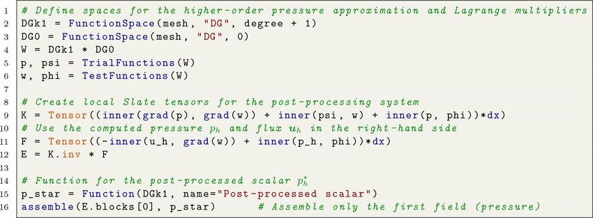
T. H. Gibson et al.: Hybridization and static condensation methods for GFD                                                                           737

Whenever the facet domain is clear by the context, we omit                  a nonlinear form corresponding to a PDE (also known as the
the subscripts for brevity and simply write [[·]].                          form Jacobian). We refer the interested reader to Alnæs et al.
                                                                            (2014, Sect. 2.1.2) for more details. For clarity, we present
                                                                            examples of multi-linear forms of arity α = 0, 1, and 2 that
2     A system for localized algebra on finite element                      frequently appear in finite element discretizations:
      tensors
                                                                                                           XZ
                                                                            a(κ; v, u) := (∇v, κ∇u)Th ≡           ∇v · (κ∇u) dx,
We present an expressive language for dense linear algebra
                                                                                                                     K∈Th K
on the elemental matrix systems arising from finite element
problems. The language, which we call Slate, provides typi-                 κ ∈ C0 , u ∈ V1 , v ∈ V0 , α = 2, q = 1,                                  (6)
cal mathematical operations performed on matrices and vec-
tors; hence the input syntax is comparable to high-level linear
algebra software such as MATLAB. The Slate language pro-                                                        XZ
vides basic abstract building blocks which can be used by a                 a(f ; v) := (v, f )Th ≡                  v f dx,
specialized compiler for linear algebra to generate low-level                                               K∈Th K
code implementations.                                                       f ∈ C0 , v ∈ V0 , α = 1, q = 1,                                           (7)
   Slate is heavily influenced by the Unified Form Language
(UFL) (Alnæs et al., 2014; Logg et al., 2012a), a DSL em-
bedded in Python which provides symbolic representations                                                                  XZ
of finite element forms. The expressions can be compiled by                 a(f, g; ) := (f − g, f − g)Th ≡                       |f − g|2 dx,
a form compiler, which translates UFL into low-level code                                                                K∈Th K
for the local assembly of a form over the cells and facets of
                                                                            g ∈ C1 , f ∈ C0 , α = 0, q = 2,                                           (8)
a mesh. In a similar manner, Slate expressions are compiled
to low-level code that performs the requested linear algebra
element-wise on a mesh.                                                                                          XZ
                                                                            a(γ , σ ) := hγ , [[σ ]]i∂ Th ≡                γ [[σ ]] ds
2.1    An overview of Slate                                                                                          ◦
                                                                                                                 e∈Eh e

To clarify conventions and the scope of Slate, we start by                      XZ
                                                                            +               γ σ · n ds, σ ∈ V1 , γ ∈ V0 , α = 2, q = 0.               (9)
establishing our notation for a general finite element form
                                                                                e∈Eh∂ e
following the convention of Alnæs et al. (2014). We define
a real-valued multi-linear form as an operator which maps a                    In general, a finite element form will consist of integrals
list of arguments v = (v0 , · · ·, vα−1 ) ∈ V0 ×· · ·×Vα−1 into R:          over various geometric domains: integration over cells Th ,
                                                                            interior facets Eh ◦ , and exterior facets Eh∂ . Therefore, we ex-
a : V0 × · · · × Vα−1 → R,        a 7 −→ a(v0 , · · ·, vα−1 ) = a(v), (4)
                                                                            press a general multi-linear form in terms of integrals over
                                                                            each set of geometric entities:
where a is linear in each argument vk . The arity of a form is
α, an integer denoting the total number of form arguments.                              XZ
                                                                                                  T
                                                                                                                XZ          ◦
In traditional finite element nomenclature (for α ≤ 2), V0 is               a(c; v) =          IK (c; v) dx +          IeE , (c; v) ds
                                                                                            K∈Th K                          ◦
referred to as the space of test functions and V1 as the space of                                                        e∈Eh e
trial functions. Each Vk are referred to as argument spaces.                    XZ
Forms with arity α = 0, 1, or 2 are best interpreted as the                 +               IeE ,∂ (c; v) ds,                                        (10)
more familiar mathematical objects: scalars (0-forms), linear                   e∈Eh∂   e
forms or functionals (1-forms), and bilinear forms (2-forms),                                                                                    ◦
                                                                            where IK T denotes a cell integrand on K ∈ T , I E , is an
respectively.                                                                                                                    h  e
   If a given form a is parameterized by one or more coef-                  integrand on the interior facet e ∈ Eh ◦ , and IeE ,∂ is an inte-
                                                                   q
ficients, say c = (c0 , · · ·, cq ) ∈ C0 × · · · × Cq , where {Ck }k=0      grand defined on the exterior facet e ∈ Eh∂ . The form a(c; v)
are coefficient spaces, then we write                                       describes a finite element form globally over the entire prob-
                                                                            lem domain.
a : C0 × · · · × Cq × V0 × · · · × Vα−1 → R,                                   Here, we will  consider the case where the interior facet in-
                                                                                          ◦
a 7 −→ a(c0 , · · ·, cq ; v0 , · · ·, vα−1 ) = a(c; v).              (5)    tegrands IeE , (c; v) can be decomposed into two independent
                                                                            parts on each interior facet e: one for the positive restriction
From here on, we shall work exclusively with forms that are                 (+) and the negative   restriction (−). That is, for each e ∈ Eh ◦ ,
                                                                                              E ,◦           E ,◦          E ,◦
linear in v and possibly nonlinear in the coefficients c. This              we may write Ie (c; v) = Ie+ (c; v) + Ie− (c; v). This al-
is reasonable since nonlinear methods based on Newton iter-                 lows us to express the integral over an interior facet e con-
ations produce linear problems via Gâteaux differentiation of               necting two adjacent elements, say K + and K − , as the sum

www.geosci-model-dev.net/13/735/2020/                                                                    Geosci. Model Dev., 13, 735–761, 2020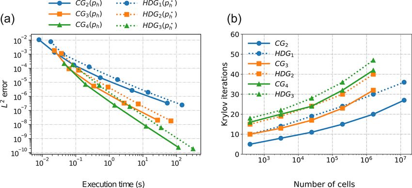
738                                                         T. H. Gibson et al.: Hybridization and static condensation methods for GFD

of integrals:                                                                 the cell-node map e(K, ·). Within Firedrake, this operation is
     Z                        Z                                               handled by PyOP2 (Rathgeber et al., 2012) and serves as the
                 ◦                                ◦
            IeE , (c; v) ds =                 IeE+, (c; v) ds                 main user-facing abstraction for global finite element assem-
                                                                              bly. For many applications, one may want to produce a new
e⊂∂K + ∪∂K −                         e⊂∂K +
      Z                                                                       global operator by algebraically manipulating different ele-
              E ,◦                                                            ment tensors. This is relatively invasive in numerical code,
+            Ie− (c; v) ds.                                           (11)
                                                                              as it requires bypassing direct operator assembly to produce
    e⊂∂K −
                                                                              the new tensor. This is precisely the scope of Slate.
The local contribution of Eq. (10) in each cell K, along with                    Like UFL, Slate relies on the grammar of the host-
its associated facets e ⊂ ∂K, is then                                         language: Python. The entire Slate language is implemented
             Z                  X Z                                           as a Python module which defines its types (classes) and op-
                 T                           ◦
aK (c; v) = IK (c; v) dx +              IeE , (c; v) ds                       erations on said types. Together, this forms a high-level lan-
                K
                                         e⊂∂K ∂ e                            guage for expressing dense linear algebra on element tensors.
               Z                                                              The Slate language consists of two primary abstractions for
                     IeE ,∂ (c; v) ds.
       X
+                                                                     (12)    linear algebra:
    e⊂∂K∩∂ e
                                                                                1. terminal element tensors corresponding to multi-linear
We call Eq. (12) the cell-local contribution of a(c; v), with                      integral forms (matrices, vectors, and scalars) or assem-
          X                                                                        bled data (for example, coefficient vectors of a finite el-
a(c; v) =     aK (c; v).                                  (13)
                                                                                   ement function) and
             K∈Th

   To make matters concrete, let us suppose a(c; v) is a bi-                    2. expressions consisting of algebraic operations on termi-
linear form with arguments v = (v0 , v1 ) ∈ V0 × V1 . Now let                      nal tensors.
{8i }N                M
     i=1 and {9i }i=1 denote bases for V0 and V1 , respec-                    The composition of binary and unary operations on terminal
tively. Then the global N × M matrix A corresponding to
                                                                              tensors produces a Slate expression. Such expressions can
a(c; v0 , v1 ) has its entries defined via
                                                                              be composed with other Slate objects in arbitrary ways, re-
                                                                              sulting in concise representations of complex algebraic op-
                           X
Aij = a c; 8i , 9j =            AK,ij , AK,ij
                               K∈Th                                           erations on locally assembled arrays. We summarize all cur-
                                                                             rently supported Slate abstractions here.
= aK c; 8i , 9j .                                                     (14)

By construction, AK,ij 6 = 0 if and only if 8i and 9j take                    2.1.1     Terminal tensors
non-zero values in K. Now we introduce the cell-node map
                                                                              In Slate, one associates a tensor with data on a cell either by
i = e(K, î) as the mapping from the local node number î in
                                                                              using a multi-linear form, or assembled coefficient data:
K to the global node number i. Suppose there are n and m
nodes defining the degrees of freedom for V0 and V1 , respec-                   – Tensor(a(c; v))
tively, in K. Then all non-zero entries of AK,ij arise from                       associates a form, expressed in UFL, with its local ele-
integrals involving basis functions with local indices corre-                     ment tensor
sponding to the global indices i, j :
                                                                                    AK ← aK (c; v), for allK ∈ Th .                        (16)
AKî jˆ
        := a K   c; 8e(K,î) , 9 e(K,j ) , î ∈ [1, · · ·, n] ,
                                     ˆ
                                                                                      The form arity α of aK (c; v) determines the rank of the
jˆ ∈ [1, · · ·, m] .                                                  (15)            corresponding Tensor; i.e., scalars, vectors, and ma-
These local contributions are collected in the n × m dense                            trices are produced from scalars, linear forms, and bilin-
matrix AK , which we call the element tensor. The global ma-                          ear forms, respectively.1 The shape of the element ten-
trix A is assembled from the collection of element tensors:                           sor is determined by both the number of arguments and
A ← {AK }K∈Th . For details on the general evaluation of fi-                          total number of degrees of freedom local to the cell.
nite element basis functions and multi-linear forms, we refer
                                                                                – AssembledVector(f ),
the reader to Kirby (2004), Kirby and Logg (2006), Logg
                                                                                  where f is some finite element function. The function
et al. (2012b), and Homolya et al. (2018). Further details on
                                                                                  f ∈ V is expressed in terms of the finite element basis
the global assembly of finite element operators, with a par-
ticular focus on code generation, are summarized in the work                     1 Similarly to UFL, Slate is capable of abstractly representing
of Logg and Wells (2010) and Markall et al. (2013).                           arbitrary rank tensors. However, only rank ≤ 2 tensors are typically
   In standard finite element software packages, the element                  used in most finite element applications, and therefore we currently
tensor is mapped entry-wise into a global sparse array using                  only generate code for those ranks.

Geosci. Model Dev., 13, 735–761, 2020                                                               www.geosci-model-dev.net/13/735/2020/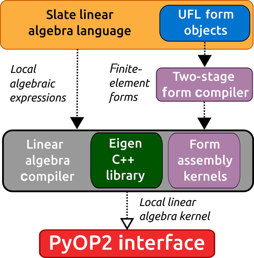
T. H. Gibson et al.: Hybridization and static condensation methods for GFD 739
of V : f (x) = N
P
i=1 fi 8i (x). The result is the local co- Each Tensor object knows all the information about the un-
efficient vector of f on K: derlying UFL form that defines it, such as form arguments,
n on coefficients, and the underlying finite element space(s) it op-
FK ← fe(K,î) , (17) erates on. This information is propagated through as unary or
î=1 binary transformations are applied. The unary and binary op-
erations shown here provide the necessary algebraic frame-
where e(K, î) is the local node numbering and n is the
work for a large class of problems, some of which we present
number of nodes local to the cell K.
in this paper.
In Firedrake, Slate expressions are transformed into low-
2.1.2 Symbolic linear algebra
level code by a linear algebra compiler. The compiler inter-
Slate supports typical binary and unary operations in linear prets Slate expressions as a syntax tree, where the tree is vis-
algebra, with a high-level syntax close to mathematics. At ited to identify what local arrays need to be assembled and
the time of this paper, these include the following. the sequence of array operations. At the time of this work,
our compiler generates C++ code, using the templated library
– A + B, the addition of two equal shaped tensors: AK + Eigen (Guennebaud et al., 2015) for dense linear algebra. The
BK . translation from Slate to C++ is fairly straightforward, as all
operations supported by Slate have a representation in Eigen.
– A ∗ B, a contraction over the last index of A and the first The compiler pass will generate a single “macro” kernel,
index of B. This is the usual multiplicative operation on which performs the dense linear algebra operations repre-
matrices, vectors, and scalars: AK BK . sented in Slate. The resulting code will also include (often
multiple) function calls to local assembly kernels generated
– -A, the additive inverse (negation) of a tensor: −AK . by TSFC (Two Stage Form Compiler) (Homolya et al., 2018)
T to assemble all necessary sub-blocks of an element tensor.
– A.T, the transpose of a tensor: AK . All code generated by the linear algebra compiler conforms
−1 to the application programming interface (API) of the PyOP2
– A.inv, the inverse of a square tensor: AK . framework, as detailed by Rathgeber et al. (2012, Sect. 3).
Figure 1 provides an illustration of the complete tool chain.
– A.solve(B, decomposition=‘‘...”), the re- Most optimization of the resulting dense linear algebra
sult, XK , of solving a local linear system AK XK = BK , code is handled directly by Eigen. In the case of unary and
optionally specifying a factorization strategy. binary operations such as A.inv and A.solve(B), sta-
ble default behaviors are applied by the linear algebra com-
– A.blocks[indices], where A is a tensor from a
piler. For example, A.solve(B) without a specified fac-
mixed finite element space. This allows for the extrac-
torization strategy will default to using an in-place LU fac-
tion of sub-blocks, which are indexed by field (slices are
torization with partial pivoting. For local matrices smaller
allowed). For example, if a matrix A corresponds to the
than 5 × 5, the inverse is translated directly into Eigen’s
bilinear form a : V × W → R, where V = V0 × · · · × Vn
A.inverse(), which employs stable analytic formulas.
and W = W0 ×· · ·×Wm are product spaces consisting of
For larger matrices, the linear algebra replaces A.inv with
finite element spaces {Vi }ni=0 , {Wi }m
i=0 , then the element an LU factorization.2 Currently, we only support direct ma-
tensors have the form
trix factorizations for solving local linear systems. However,
AK AK ··· AK
it would not be difficult to extend Slate to support more gen-
00 01 0m
eral solution techniques like iterative methods.
AK 10 AK 11 ··· AK
1m
AK = . (18)
.. .. .. ..
. . . .
3 Examples
AKn0 AKn1 ··· K
Anm
We now present examples and discuss solution methods
The associated submatrix of Eq. (18) with indices i =
which require element-wise manipulations of finite element
(p, q), p = {p1 , · · ·, pr }, q = {q1 , · · ·, qc }, is
systems and their specification in Slate. We stress here that
Slate is not limited to these model problems; rather these ex-
AK AK
p1 q1 ··· p1 qc amples are chosen for clarity and to demonstrate key fea-
AK .. .. .. K
tures of the Slate language. For our discussion, we use a
= = A .blocks[p, q],
pq . . .
AK ··· AK model elliptic equation defined in a computational domain
pr q1 pr qc
(19) 2 For more details on solving linear equations in Eigen, see https:
//eigen.tuxfamily.org/dox/group__TutorialLinearAlgebra.html (last
where p ⊆ {0, · · ·, n}, q ⊆ {0, · · ·, m}. access: 3 January 2020).
www.geosci-model-dev.net/13/735/2020/ Geosci. Model Dev., 13, 735–761, 2020
740                                               T. H. Gibson et al.: Hybridization and static condensation methods for GFD

                                                                       spaces Uh × Vh ⊂ H (div; ) × L2 (), defined by

                                                                       Uh = {w ∈ H (div; ) : w|K ∈ U (K), ∀K ∈ Th ,
                                                                       w · n = g on ∂N } ,                                            (27)

                                                                           n                                 o
                                                                       Vh = φ ∈ L2 () : φ|K ∈ V (K), ∀K ∈ Th .                        (28)

                                                                       The space Uh consists of H (div)-conforming piecewise
                                                                       vector polynomials, where choices of U (K) typically in-
                                                                       clude the Raviart–Thomas (RT), Brezzi–Douglas–Marini
                                                                       (BDM), or Brezzi–Douglas–Fortin–Marini (BDFM) ele-
                                                                       ments (Raviart and Thomas, 1977; Nédélec, 1980; Brezzi
                                                                       et al., 1985, 1987). The space Vh is the Lagrange family of
                                                                       discontinuous polynomials. These spaces are of particular in-
                                                                       terest when simulating geophysical flows, since choosing the
                                                                       right pairing results in stable discretizations with desirable
                                                                       conservation properties and avoids spurious computational
                                                                       modes. We refer the reader to Cotter and Shipton (2012),
Figure 1. The Slate language wraps UFL objects describing the
                                                                       Cotter and Thuburn (2014), Natale et al. (2016), and Ship-
finite element system. The resulting Slate expressions are passed
to a specialized linear algebra compiler, which produces a single
                                                                       ton et al. (2018) for a discussion of mixed methods relevant
macro kernel assembling the local contributions and executes the       for geophysical fluid dynamics. Two examples of such dis-
dense linear algebra represented in Slate. The kernels are passed to   cretizations are presented in Sect. 5.2.
the Firedrake’s PyOP2 interface, which wraps the Slate kernel in          The mixed formulation of Eqs. (23)–(26) is arrived at by
a mesh-iteration kernel. Parallel scheduling, code generation, and     multiplying Eqs. (23)–(24) by test functions and integrating
compilation occurs after the PyOP2 layer.                              by parts. The resulting finite element problem reads as fol-
                                                                       lows: find (uh , ph ) ∈ Uh × Vh satisfying

. Consider the second-order PDE with both Dirichlet and               (w, µuh )Th − (∇ · w, ph )Th = −hw · n, p0 i∂D ,
Neumann boundary conditions:                                           ∀w ∈ Uh,0 ,                                                     (29)

−∇ · (κ∇p) + cp = f, in ,                                     (20)
p = p0 , on ∂D ,                                              (21)
−κ∇p · n = g, on ∂N ,                                         (22)    (φ, ∇ · uh )Th + (φ, cph )Th = (φ, f )Th , ∀φ ∈ Vh ,            (30)

where ∂D ∪ ∂N = ∂ and κ, c :  → R+ are positive-                   where Uh,0 is the subspace of Uh with functions whose nor-
valued coefficients. To obtain a mixed formulation of                  mal components vanish on ∂N . The discrete system is ob-
Eqs. (20)–(22), we introduce the auxiliary velocity variable           tained by first expanding the solutions in terms of the finite
u = −κ∇p. We then obtain the first-order system of PDEs:               element bases:

                                                                              Nu                    Np
µu + ∇p = 0, in ,                                             (23)           X                     X
                                                                       uh =         Ui 9 i , ph =         Pi ξi ,                      (31)
∇ · u + cp = f, in ,                                          (24)           i=1                   i=1
p = p0 , on ∂D ,                                              (25)
                                                                                                     N
u · n = g, on ∂N ,                                            (26)    where {9 i }N u              p
                                                                                   i=1 and {ξi }i=1 are bases for Uh and Vh , respec-
                                                                       tively. Here, Ui and Pi are the coefficients to be determined.
where µ = κ −1 .                                                       As per standard Galerkin-based finite element methods, tak-
                                                                       ing w = 9 j , j ∈ {1, · · ·, Nu } and φ = ξj , j ∈ {1, · · ·, Np } in
3.1   Hybridization of mixed methods                                   Eqs. (29)–(30) produces the following discrete saddle point
                                                                       system:
To motivate our discussion in this section, we start by recall-
                                                                           A −BT

ing the mixed method for Eqs. (23)–(26). Methods of this                                   U     F0
type seek approximations (uh , ph ) in finite-dimensional sub-                                =       .                                (32)
                                                                           B D             P     F1

Geosci. Model Dev., 13, 735–761, 2020                                                        www.geosci-model-dev.net/13/735/2020/
T. H. Gibson et al.: Hybridization and static condensation methods for GFD 741
Nu p N
where U = {Ui }i=1 , P = {Pi }i=1 are the coefficient vectors, called the transmission condition, is added to close the sys-
and tem. The resulting hybridizable formulation reads as follows:
find (udh , ph , λh ) ∈ Uhd × Vh × Mh such that
Aij = 9 i , µ9 j T , (33)
h
Bij = ξi , ∇ · 9 j T , (34) w, µudh − (∇ · w, ph )Th + h[[w]] , λh i∂ Th r∂D
h Th
Dij = ξi , cξj T , (35) = −hw · n, p0 i∂D , ∀w ∈ Uhd , (41)
h
F0,j = − 9 j · n, p0 ∂D
, (36)
F1,j = ξj , f T . (37)
h
φ, ∇ · udh + (φ, cph )Th = (φ, f )Th , ∀φ ∈ Vh , (42)
Methods to efficiently invert such systems include H (div)- Th
multigrid (Arnold et al., 2000) (requiring complex overlap-
ping Schwarz smoothers), global Schur complement factor- D hh iiE
izations (which require an approximation to the inverse of γ , udh = hγ , gi∂N , ∀γ ∈ Mh,0 , (43)
∂ Th r∂D
the dense3 elliptic Schur complement D + BA−1 BT ), or aux-
iliary space multigrid (Hiptmair and Xu, 2007). Here, we fo- where Mh,0 denotes the space of traces vanishing on ∂D .
cus on a solution approach using a hybridized mixed method The transmission condition Eq. (43) enforces both the con-
(Arnold and Brezzi, 1985; Brezzi and Fortin, 1991; Boffi tinuity of udh · n across element boundaries as well as the
et al., 2013). boundary condition udh · n = g on ∂N . If the space of La-
The hybridization technique replaces the original system grange multipliers Mh is chosen appropriately, then the bro-
with a discontinuous variant, decoupling the velocity degrees ken velocity udh , albeit sought a priori in a discontinuous
of freedom between cells. This is done by replacing the dis- space, will coincide with its H (div)-conforming counterpart.
crete solution space for uh with the “broken” space Uhd , de- Specifically, the formulations in Eqs. (41)–(42) and (29)–
fined as (30) are solving equivalent problems if the normal compo-
n h in o nents of w ∈ Uh lie in the same polynomial space as the trace
Uhd = w ∈ L2 () : w|K ∈ U (K), ∀K ∈ Th . (38) functions (Arnold and Brezzi, 1985).
n The discrete matrix system arising from Eqs. (41)–(43) has
The vector finite element space Uhd is a subspace of L2 ()
the general form
consisting of local H (div) functions, but normal components
A00 A01 A02 Ud F0
are no longer required to be continuous on ∂Th . The approx-
imation space for ph remains unchanged. A10 A11 A12 P = F1 , (44)
A20 A21 A22 3 F2
Next, Lagrange multipliers are introduced as an auxiliary
variable in the space Mh , defined only on cell interfaces:
where the discrete system is produced by expanding func-
Mh = {γ ∈ L2 (∂Th ) : γ |e ∈ M(e), ∀e ∈ ∂Th }, (39) tions in terms of the finite element bases for Uhd , Vh , and Mh
like before. Upon initial inspection, it may not appear to be
where M(e) denotes a polynomial space defined on each advantageous to replace our original formulation with this
facet. We call Mh the space of approximate traces. Functions augmented equation set; the hybridizable system has sub-
in Mh are discontinuous across vertices in two dimensions stantially more total degrees of freedom. However, Eq. (44)
and vertices or edges in three dimensions. has a considerable advantage over Eq. (32) in the following
Deriving the hybridizable mixed system is accomplished ways.
through integration by parts over each element K. Testing
with w ∈ Uhd (K) and integrating Eq. (23) over the cell K 1. Since both Uhd and Vh are discontinuous spaces, Ud and
produces P are coupled only within the cell. This allows us to
simultaneously eliminate both unknowns via local static
w, µudh − (∇ · w, ph )K + hw · n, λh i∂K condensation to produce a significantly smaller global
K (hybridized) problem for the trace unknowns, 3:
= −hw · n, p0 i∂K∩∂D . (40)
S3 = E, (45)
The trace function λh is introduced in the surface integral as
an approximation to p|∂K . An additional constraint equation, where S ← {SK }K∈Th and E ← {EK }K∈Th are assem-
bled via the local element tensors:
3 The Schur complement, while elliptic, is globally dense due to
" #−1 " #
the fact that A has a dense inverse. This is a result of velocities in h i AK AK AK
SK = AK
22 − AK AK 00 01 02 , (46)
Uh having continuous normal components across cell interfaces. 20 21 AK
10 AK
11 AK
12
www.geosci-model-dev.net/13/735/2020/ Geosci. Model Dev., 13, 735–761, 2020
742                                                           T. H. Gibson et al.: Hybridization and static condensation methods for GFD

                                                                                   Deriving the LDG-H formulation follows exactly from
                                      "               #−1 (      )              standard DG methods. All prognostic variablesnare sought
                                          AK    AK            FK
                                                                                in the discontinuous spaces Uh × Vh ⊂ L2 () × L2 ().
                  h               i
      EK = FK
            2 −       AK    AK             00    01            0 .      (47)
                       20    21           AK
                                           10   AK
                                                 11           FK
                                                               1                Within a cell K, integration by parts yields
      Note that the inverse of the block matrix in Eqs. (46) and
                                                                                (w, µuh )K − (∇ · w, ph )K + hw · n, p
                                                                                                                     bi∂K = 0,
      (47) is never evaluated globally; the elimination can be
      performed locally by performing a sequence of Schur                       ∀w ∈ U (K),                                                (50)
      complement reductions within each cell.
 2. The matrix S is sparse, symmetric, positive-definite, and
                                                                                − (∇φ, uh )K + hφ,b
                                                                                                  u · ni∂K + (φ, cph )K = (φ, f )K ,
    spectrally equivalent to the dense Schur complement
    D+BA−1 BT from Eq. (32) of the original mixed formu-                        ∀φ ∈ V (K),                                                (51)
    lation (Gopalakrishnan, 2003; Cockburn et al., 2009a).
                                                                                where U (K) and V (K) are vector and scalar polynomial
 3. Once 3 is computed, both Ud and P can be recovered                          spaces, respectively. Now, we define the numerical fluxes p
                                                                                                                                          b
    locally in each element. This can be accomplished in a                          u to be functions of the trial unknowns and a new inde-
                                                                                and b
    number of ways. One way is to compute PK by solving                         pendent unknown in the trace space Mh :
                    −1
        K      K
      A11 − A10 A00 K
                           A01 PK = FK
                             K                    K                             u(uh , ph , λh ; τ ) = uh + τ (ph − p
                                                                                                                    b) n,                  (52)
                                           1 − A10
                                                                                b
                                                                              p
                                                                                b(λh ) = λh ,                                              (53)
         −1                           −1
      AK
       00     FK
               0 −    A K
                        12 − A K
                               10   A K
                                      00     A K    K
                                               02 3 , (48)                      where λh ∈ Mh is a function approximating p on ∂Th and
                                                                                τ is a positive stabilization function that may vary on each
                                K
      followed by solving for Ud :                                              facet e ∈ ∂Th . We further require that λh satisfies the Dirich-
           K                                                                  let condition for p on ∂D in an L2 -projection sense. The
      AK     d
                 = FK       K K    K K                                          full LDG-H formulation reads as follows. Find (uh , ph , λh ) ∈
        00 U         0 − A01 P − A02 3 .                                (49)
                                                                                Uh × Vh × Mh such that
      Similarly, one could rearrange the order in which each
                                                                                (w, µuh )Th − (∇ · w, ph )Th + h[[w]] , λh i∂ Th = 0,
      variable is reconstructed.
                                                                                ∀w ∈ Uh ,                                                  (54)
 4. If desired, the solutions can be improved further through
    local post-processing. We highlight two such proce-
    dures for Ud and P, respectively, in Sect. 3.3.
                                                                                − (∇φ, uh )Th + φ, uh + τ (ph − λh ) n ∂ T
                                                                                                                                  h
   Figure 2 displays the corresponding Slate code for assem-
bling the trace system, solving Eq. (45), and recovering the                    + (φ, cph )Th = (φ, f )Th , ∀φ ∈ Vh ,                      (55)
eliminated unknowns. For a complete reference on how to
formulate the hybridized mixed system Eqs. (41)–(43) in
UFL, we refer the reader to Alnæs et al. (2014). Complete                        γ , uh + τ (ph − λh ) n ∂ T            = hγ , gi∂N ,
                                                                                                               h r∂D
Firedrake code using Slate to solve a hybridizable mixed sys-                   ∀γ ∈ Mh ,                                                  (56)
tem is also publicly available in Zenodo/Tabula-Rasa (2019,
“Code verification”). We remark that, in the case of this
hybridizable system, Eq. (44) contains zero-valued blocks
which can simplify the resulting expressions in Eqs. (46)–                      hγ , λh i∂D = hγ , p0 i∂D , ∀γ ∈ Mh .                    (57)
(47) and (48)–(49). This is not true in general and therefore
the expanded form using all sub-blocks of Eq. (44) is pre-                      Equation (56) is the transmission condition, which enforces
sented for completeness.                                                        the continuity of bu ·n on ∂Th and q. Equation (57) ensures λh
                                                                                satisfies the Dirichlet condition. This ensures that the numer-
3.2   Hybridization of discontinuous Galerkin methods                           ical flux is single-valued on the facets. Hence, the LDG-H
                                                                                method defines a conservative DG method (Cockburn et al.,
The HDG method is a natural extension of discontinuous                          2010b). Note that the choice of τ has a significant influence
Galerkin (DG) discretizations. Here, we consider a specific                     on the expected convergence rates of the computed solutions.
HDG discretization, namely the LDG-H method (Cockburn                              The LDG-H method retains the advantages of standard DG
et al., 2010b). Other forms of HDG that involve local lifting                   methods while also enabling the assembly of reduced linear
operators can also be implemented in this software frame-                       systems through static condensation. The matrix system aris-
work by the introduction of additional local (i.e., discontinu-                 ing from Eqs. (54)–(57) has the same general form as the hy-
ous) variables into the definition of the local solver.                         bridized mixed method in Eq. (44), except all sub-blocks are

Geosci. Model Dev., 13, 735–761, 2020                                                               www.geosci-model-dev.net/13/735/2020/
T. H. Gibson et al.: Hybridization and static condensation methods for GFD 743
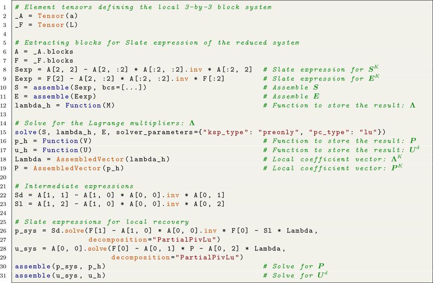
Figure 2. Firedrake code for solving Eq. (44) via static condensation and local recovery, given UFL expressions a, L for Eqs. (41)–(43).
Arguments of the mixed space Uhd × Vh × Mh are indexed by 0, 1, and 2, respectively. Lines 8 and 9 are symbolic expressions for Eqs. (46)
and (47), respectively. Any vanishing conditions on the trace variables should be provided as boundary conditions during operator assembly
(line 10). Lines 26 and 28 are expressions for Eqs. (48) and (49) (using LU). Code generation occurs in lines 10, 11, 30, and 31. A global
linear solver for the reduced system is created and used in line 15. Configuring the linear solver is done by providing an appropriate Python
dictionary of solver options for the PETSc library.
now populated with non-zero entries due to the coupling of previous discussions in Sect. 3.1 and 3.2, using the standard
trace functions with both ph and uh . However, all previous set of operations on element tensors summarized in Sect. 2.1.
properties of the discrete matrix system from Sect. 3.1 still
apply. The Slate expressions for the local elimination and re-
construction operations will be identical to those illustrated
in Fig. 2. For the interested reader, a unified analysis of hy-
bridization methods (both mixed and DG) for second-order
elliptic equations is presented in Cockburn et al. (2009a) and 3.3.1 Post-processing of the scalar solution
Cockburn (2016).
3.3 Local post-processing
Our first example is a modified version of the procedure pre-
For both mixed (Arnold and Brezzi, 1985; Brezzi et al., 1985; sented by Stenberg (1991) for enhancing the accuracy of the
Bramble and Xu, 1989; Stenberg, 1991) and discontinuous scalar solution. This was also highlighted within the context
Galerkin methods (Cockburn et al., 2010b, 2009b), it is pos- of hybridizing eigenproblems by Cockburn et al. (2010a).
sible to locally post-process solutions to obtain superconver- This post-processing technique can be used for both the hy-
gent approximations (gaining 1 order of accuracy over the bridizable mixed and LDG-H methods. We proceed by pos-
unprocessed solution). These methods can be expressed as ing the finite element systems cell-wise.
local solves on each element and are straightforward to im- Let Pk (K) denote a polynomial space of degree ≤ k on
plement using Slate. In this section, we present two post- a cell K ∈ Th . Then for a given pair of computed solu-
processing techniques: one for scalar fields and another for tions uh , ph of the hybridized methods, we define the post-
the vector unknown. The Slate code follows naturally from processed scalar ph? ∈ Pk+1 (K) as the unique solution of the
www.geosci-model-dev.net/13/735/2020/ Geosci. Model Dev., 13, 735–761, 2020744 T. H. Gibson et al.: Hybridization and static condensation methods for GFD
local problem: satisfying
n
r, u?h K = (r, uh )K , ∀r ∈ Pk−1 (K) ,
⊥,l (62)
∇w, ∇ph? K = − ∇w, κ −1 uh , ∀w ∈ Pk+1
(K), (58)
K µ, u?h · n e = hµ,b
u · nie , ∀µ ∈ Pk (e) (63)
v, ph? K = (v, ph )K , ∀v ∈ Pl (K),
(59)
for all facets e on ∂K, where bu is the numerical flux defined
⊥,l
in Eq. (52). This local problem produces a new velocity u?h
where 0 ≤ l ≤ k. Here, the space Pk+1 (K) denotes the with the following properties.
2
L -orthogonal complement of Pl (K). This post-processing
method directly uses the definition of the flux uh , the approx- 1. u?h converges at the same rate as uh for all choices of τ
⊥,l producing a solvable system for Eqs. (54)–(57). How-
imation of −κ∇p. In practice, the space Pk+1 (K) may be
constructed using an orthogonal hierarchical basis, and solv- ever,
ing Eqs. (58)–(59) amounts to inverting a symmetric positive
2. u?h ∈ H (div; ). That is, u?h e = 0, ∀e ∈ Eh ◦ .
definite system in each cell of the mesh.
At the time of this work, Firedrake does not support the 3. Additionally, the divergence of u?h convergences at a
construction of such a finite element basis. However, we can rate of k + 1.
introduce Lagrange multipliers to enforce the orthogonality
constraint. The resulting local problem then becomes the fol- The Firedrake implementation using Slate is similar to the
lowing mixed system: find (ph? , ψ) ∈ Pk+1 (K)×Pl (K) such scalar post-processing example (see Fig. 3); the cell-wise lin-
that ear systems Eqs. (62)–(63) can be expressed in UFL, and
therefore the necessary Slate expressions to invert the lo-
∇w, ∇ph?
+ (w, ψ)K = − ∇w, κ −1 uh , cal systems follows naturally from the set of operations pre-
K K sented in Sect. 2.1. We use the very sensitive parameter de-
∀w ∈ Pk+1 (K), (60) pendency in the post-processing methods to validate our soft-
ware implementation in Zenodo/Tabula-Rasa (2019, “Code-
verification”).
φ, ph?
K
= (φ, ph )K , ∀φ ∈ Pl (K), (61) 4 Static condensation as a preconditioner
Slate enables static condensation approaches to be expressed
where 0 ≤ l ≤ k. The local problems Eqs. (60)–(61) and
very concisely. Nonetheless, the application of a particular
Eqs. (58)–(59) are equivalent, with the Lagrange multiplier
approach to different variational problems using Slate still
ψ enforcing orthogonality of test functions in Pk+1 (K) with
requires a certain amount of code repetition. By formulating
functions in Pl (K).
each form of static condensation as a preconditioner, code
This post-processing method produces a new approxima-
can be written once and then applied to any mathematically
tion which superconverges at a rate of k + 2 for hybridized
suitable problem. Rather than writing the static condensation
mixed methods (Stenberg, 1991; Cockburn et al., 2010a).
by hand, in many cases, it is sufficient to just select the ap-
For the LDG-H method, k + 2 superconvergence is achieved
propriate, Slate-based, preconditioner.
when τ = O(1) and τ = O(h), but only k + 1 convergence is
For context, it is helpful to frame the problem in the par-
achieved when τ = O(1/ h) (Cockburn et al., 2009b, 2010b).
ticular context of the solver library: PETSc. Firedrake uses
We demonstrate the increased accuracy in computed solu-
PETSc as its main solver abstraction framework and can pro-
tions in Sect. 5.1. An abridged example using Firedrake and
vide operator-based preconditioners for solving linear sys-
Slate to solve the local linear systems is provided in Fig. 3.
tems as PC objects expressed in Python via petsc4py (Dalcin
et al., 2011). For a comprehensive overview on solving linear
3.3.2 Post-processing of the flux
systems using PETSc, we refer the interested reader to Balay
et al. (2019, Sect. 4).
Our second example illustrates a procedure that uses the nu-
Suppose we wish to solve a linear system: Ax = b. We can
merical flux of an HDG discretization for Eqs. (23)–(26).
think of (left) preconditioning the system in residual form:
Within the context of the LDG-H method, we can use the
numerical trace in Eq. (52) to produce a vector field that is r = r(A, b) ≡ b − Ax = 0 (64)
H (div)-conforming. The technique we outline here follows
that of Cockburn et al. (2009b). by an operator P (which may not necessarily be linear) as a
Let Th be a mesh consisting of simplices. On each cell transformation into an equivalent system of the form
K ∈ Th , we define a new function u?h to be the unique ele-
ment of the local Raviart–Thomas space [Pk (K)]n +xPk (K) Pr = Pb − PAx = 0. (65)
Geosci. Model Dev., 13, 735–761, 2020 www.geosci-model-dev.net/13/735/2020/T. H. Gibson et al.: Hybridization and static condensation methods for GFD 745
Figure 3. Example of local post-processing using Firedrake and Slate. Here, we locally solve the mixed system defined in Eqs. (58)–(59).
The corresponding symbolic local tensors are defined in lines 9 and 11. The Slate expression for directly inverting the local system is written
in line 12. In line 16, a Slate-generated kernel is produced which solves the resulting linear system in each cell. Since we are not interested
in the multiplier, we only return the block corresponding to the new pressure field.
Given a current iterate xi the residual at the ith iteration is latter as a preconditioner is the ability to switch out the solu-
simply ri ≡ b−Axi , and P acts on the residual to produce an tion scheme for the system, even when nested inside a larger
approximation to the error i ≡ x − xi . If P is an application set of coupled equations or nonlinear solver (Newton-based
of an exact inverse, the residual is converted into an exact (up methods) at runtime.
to numerical roundoff) error.
We will denote the application of a particular Krylov 4.1.1 A static condensation interface for hybridization
subspace method (KSP) for the linear system Eq. (64) as
Kx (r(A, b)). Upon preconditioning the system via P as in As discussed in Sect. 3.1 and 3.2, one of the main advantages
Eq. (65), we write of using a hybridizable variant of a DG or mixed method
is that such systems permit the use of cell-wise static con-
Kx (Pr(A, b)). (66) densation. To facilitate this, we provide a PETSc PC static
If Eq. (66) is solved directly via P = A−1 , then Pr(A, b) = condensation interface: firedrake.SCPC. This precondi-
A−1 b − x. So Eq. (66) then becomes Kx (r(I, A−1 b)), pro- tioner takes the discretized system as in Eq. (44) and per-
ducing the exact solution of Eq. (64) in a single iteration of forms the local elimination and recovery procedures. Slate
K. Having established notation, we now present our imple- expressions are generated from the underlying UFL problem
mentation of static condensation via Slate by defining the ap- description.
propriate operator, P. More precisely, the incoming system has the form
4.1 Interfacing with PETSc via custom preconditioners Ae,e Ae,c Xe Re
= , (67)
Ac,e Ac,c Xc Rc
The implementation of preconditioners for the systems con-
sidered in this paper requires the manipulation not of assem- where Xe is the vector of unknowns to be eliminated, Xc
bled matrices but rather their symbolic representation. To do is the vector of unknowns for the condensed field, and
this, we use the preconditioning infrastructure developed by Re and Rc are the incoming right-hand sides. The par-
Kirby and Mitchell (2018), which gives preconditioners writ- titioning in Eq. (67) is determined by the solver option:
ten in Python access to the symbolic problem description. In pc_sc_eliminate_fields. Field indices are provided
Firedrake, this means all derived preconditioners have direct in the same way one configures solver options to PETSc.
access to the UFL representation of the PDE system. From These indices determine which field(s) to statically condense
this mathematical specification, we manipulate this appropri- into. For example, on a three-field problem (with indices 0, 1,
ately via Slate and provide operators assembled from Slate and 2), setting -pc_sc_eliminate_fields 0,1 will
expressions to PETSc for further algebraic preconditioning. configure firedrake.SCPC to cell-wise eliminate fields
Using this approach, we have developed a static condensa- 0 and 1; the resulting condensed system is associated with
tion interface for the hybridization of H (div) × L2 mixed field 2.
problems and a generic interface for statically condensing The firedrake.SCPC preconditioner can be inter-
finite element systems. The advantage of writing even the preted as a Schur complement method for Eq. (67) of the
www.geosci-model-dev.net/13/735/2020/ Geosci. Model Dev., 13, 735–761, 2020746 T. H. Gibson et al.: Hybridization and static condensation methods for GFD
form are the hybridizable (discontinuous) unknowns to be deter-
A−1 mined and CbX = Rg is the matrix representation of the trans-
P= I −A−1
e,e Ae,c e,e 0 I 0
, (68)
0 I 0 S−1 −Ac,e A−1
e,e I mission condition for the hybridizable mixed method (see
Eq. 43).
where S = Ac,c − Ac,e A−1 e,e Ae,c is the Schur complement op-
The application of firedrake.HybridizationPC
erator for the Xc system. The distinction here from block
can be interpreted as the Schur complement reduction of
preconditioners via the PETSc fieldsplit option (Brown
Eq. (70):
et al., 2012), for example, is that P does not require global
actions; by design A−1 e,e can be inverted locally and S is
I −bA−1 CT
A−1
b 0
I 0
sparse. As a result, S can be assembled or applied exactly, P
b=
A−1
, (71)
0 I 0 S−1 −Cb I
up to numerical roundoff, via Slate-generated kernels.
In practice, the only globally coupled system requiring it- where S is the Schur complement matrix S = −Cb A−1 CT .
erative inversion is S: As before, a single global system for 3 can be assem-
bled cell-wise using Slate-generated kernels. Configuring the
KXc (P1 r (S, Rs )) , (69) solver for inverting S is done via the PETSc options prefix:
where Rs = Rc − Ac,e A−1 e,e Re is the condensed right-hand -hybridization. The recovery of Ud and P happens in
side and P1 is a preconditioner for S. Once Xc is com- the same manner as firedrake.SCPC.
puted, Xe is reconstructed by inverting the system Xe = Since the hybridizable flux solution is constructed in the
A−1 broken H (div) space Uhd , we must project the computed so-
e,e Rc − Ae,c Xc cell-wise.
By construction, this preconditioner is suitable for both lution into Uh ⊂ H (div). This can be done cheaply via local
hybridized mixed and HDG discretizations. It can also be facet averaging. The resulting solution is then updated via
used within other contexts, such as the static condensa- U ← 5div Ud , where 5div : Uhd → Uh is a projection opera-
tion of continuous Galerkin discretizations (Guyan, 1965; tor. This ensures that the residual for the original mixed prob-
Irons, 1965) or primal-hybrid methods (Devloo et al., 2018). lem is properly evaluated to test for solver convergence. With
As with any PETSc preconditioner, solver options can be P
b as in Eq. (71), the preconditioning operator for the original
specified for inverting S via the appropriate options prefix system AX = R then has the form
(condensed_field). The resulting KSP for Eq. (69) is
compatible with existing solvers and external packages pro- T 5div 0 0
P = 5P5 , 5 =
b . (72)
vided through the PETSc library. This allows users to ex- 0 I 0
periment with a direct method and then switch to a more We note here that assembly of the right-hand side for the
parallel-efficient iterative solver without changing the core 3 system requires special attention. Firstly, when Neumann
application code. conditions are present, then Rg is not necessarily 0. Since the
hybridization preconditioner has access to the entire Python
4.1.2 Preconditioning mixed methods via hybridization
context (which includes a list of boundary conditions and the
The preconditioner firedrake.HybridizationPC spaces in which they are applied), surface integrals on the
expands on the previous one, this time taking an H (div)×L2 exterior boundary are added where appropriate and incorpo-
system and automatically forming the hybridizable problem. rated into the generated Slate expressions. A more subtle is-
This is accomplished through manipulating the UFL objects sue that requires extra care is the incoming right-hand side
representing the discretized PDE. This includes replacing ar- tested in the H (div) space Uh .
gument spaces with their discontinuous counterparts, intro- The situation we are given is that we have RU = RU (w)
ducing test functions on an appropriate trace space, and pro- for w ∈ Uh but require b RU (wd ) for wd ∈ Uhd . For consis-
viding operators assembled from Slate expressions in a sim- tency, we also require for any w ∈ Uh that
ilar manner as described in Sect. 4.1.1. RU (w) = RU (w).
b (73)
More precisely, let AX = R be the incoming mixed saddle
point problem, where R = RU RP T , X = U PT , and We can construct such an bRU satisfying Eq. (73) in the fol-
U and P are the velocity and scalar unknowns, respectively. lowing way. By construction, we have for each basis function
Then this preconditioner replaces AX = R with the extended 9 i ∈ Uh
problem: d
9i 9 i associated with an exterior,
A CT
b X
b R
b
= (70)
facet node
C 0 3 Rg
9 d,+ + 9 d,−
9 i associated with an interior,
i i
where 3 are the Lagrange multipliers, bR= b RU RP T , b RU 9i = facet node
and RP are the right-hand sides for the flux and scalar equa- 9 di
9 i associated with a cell,
tions, respectively, andb
· indicates modified matrices and co-
interior node
X = Ud PT
vectors with discontinuous functions. Here, b
,
Geosci. Model Dev., 13, 735–761, 2020 www.geosci-model-dev.net/13/735/2020/T. H. Gibson et al.: Hybridization and static condensation methods for GFD 747
(74) mixed problem:
where 9 di , 9 d,±
i ∈ Uhd , and 9 id,± are basis functions corre- u + ∇p = 0, (78)
sponding to the positive and negative restrictions associated
∇ · u + p = f, (79)
with the ith facet node.4 We then define our broken right-
hand side via the local definition: p = g, on ∂. (80)
RU (9 i )
RU (9 di ) =
b , (75) We start with linear polynomial approximations, up to cu-
Ni bic, for the LDG-H discretization of Eqs. (78)–(80). Addi-
tionally, we compute a post-processed scalar approximation
where Ni is the number of cells that the degree of freedom
ph? of the HDG solution. This raises the approximation order
corresponding to 9 i ∈ Uh is topologically associated with.
of the computed solution by an additional degree. In all nu-
Using Eq. (74), Eq. (75), and the fact that RU is linear in its
merical studies here, we set the HDG parameter τ = 1. All
argument, we can verify that our construction of b RU satis-
results were computed in parallel, utilizing a single compute
fies Eq. (73).
node (described previously).
A continuous Galerkin (CG) discretization of the primal
problem Eqs. (76)–(77) serves as a reference for this experi-
5 Numerical studies
ment. Due to the superconvergence in the post-processed so-
We now present results utilizing the Slate DSL and our static lution for the HDG method, we use CG discretizations of
condensation preconditioners for a set of test problems. Since polynomial orders 2, 3, and 4. This takes into account the en-
we are using the interfaces outlined in Sect. 4, Slate is ac- hanced accuracy of the HDG solution, despite being initially
cessed indirectly and requires no manually written solver computed as a lower-order approximation. We therefore ex-
code for hybridization or static condensation or local recov- pect both methods to produce equally accurate solutions to
ery. All parallel results were obtained on a single fully loaded the model problem.
compute node of dual-socket Intel E5-2630v4 (Xeon) pro- Our aim here is not to compare the performance of HDG
cessors with 2 × 10 cores (2 threads per core) running at and CG, which has been investigated elsewhere (for exam-
2.2GHz. In order to avoid potential memory effects due to ple, see Kirby et al., 2012; Yakovlev et al., 2016). Instead,
the operating system migrating processes between sockets, we provide a reference that the reader might be more famil-
we pin MPI processes to cores. iar with in order to evaluate whether our software framework
The verification of the generated code is performed us- produces a sufficiently performant HDG implementation rel-
ing parameter-sensitive convergence tests. The study consists ative to what might be expected.
of running a variety of discretizations spanning the methods To invert the CG system, we use a conjugate gradient
outlined in Sect. 3. Details and numerical results are made solver with Hypre’s BoomerAMG implementation of alge-
public and can be viewed in Zenodo/Tabula-Rasa (2019) (see braic multigrid (AMG) as a preconditioner (Falgout et al.,
“Code and data availability”). All results are in full agree- 2006). For the HDG method, we use the preconditioner de-
ment with the theory. scribed in Sect. 4.1.1 and the same solver setup as the CG
method for the trace system. While the trace operator is in-
5.1 HDG method for a three-dimensional elliptic deed symmetric and positive-definite, one should keep in
equation mind that conclusions regarding the performance of off-the-
shelf AMG packages on the HDG trace system are still rel-
In this section, we take a closer look at the LDG-H method atively unclear. As a result, efforts on developing more ef-
for the model elliptic equation (sign-definite Helmholtz): ficient multigrid strategies are a topic of ongoing interest
(Cockburn et al., 2014; Kronbichler and Wall, 2018).
− ∇ · ∇p + p = f, in = [0, 1]3 , (76) To avoid over-solving, we iterate to a relative tolerance
p = g, on ∂, (77) such that the discretization error is minimal for a given mesh.
In other words, the solvers are configured to terminate when
where f and g are chosen such that the analytic solu- there is no further reduction in the L2 error of the computed
tion is p = exp{sin(π x) sin(πy) sin(π z)}. We use a regu- solution compared with the analytic solution. This means we
lar mesh consisting of 6 · N 3 tetrahedral elements (N ∈ are not iterating to a fixed solver tolerance across all mesh
{4, 8, 16, 32, 64}). First, we reformulate Eqs. (76)–(77) as the resolutions. Therefore, we can expect the total number of
Krylov iterations (for both the CG and HDG methods) to in-
4 These are the two broken parts of 9 on a particular facet con-
i
crease as the mesh resolution becomes finer. The rationale
necting two elements. That is, for two adjacent cells, a basis func- behind this approach is to directly compare the execution
tion in Uh for a particular facet node can be decomposed into two time to solve for the best possible approximation to the solu-
basis functions in Uhd defined on their respective sides of the facet. tion given a fixed resolution.
www.geosci-model-dev.net/13/735/2020/ Geosci. Model Dev., 13, 735–761, 2020You can also read