Sensitivity study on the main tidal constituents of the Gulf of Tonkin by using the frequency-domain tidal solver in T-UGOm
←
→
Page content transcription
If your browser does not render page correctly, please read the page content below
Geosci. Model Dev., 13, 1583–1607, 2020
https://doi.org/10.5194/gmd-13-1583-2020
© Author(s) 2020. This work is distributed under
the Creative Commons Attribution 4.0 License.

Sensitivity study on the main tidal constituents of the Gulf of Tonkin
by using the frequency-domain tidal solver in T-UGOm
Violaine Piton1,2 , Marine Herrmann1,2 , Florent Lyard1 , Patrick Marsaleix3 , Thomas Duhaut3 , Damien Allain1 , and
Sylvain Ouillon1,2
1 LEGOS   UMR5566, IRD, CNRS, University of Toulouse, 31400 Toulouse, France
2 LOTUS   Laboratory, University of Science and Technology of Hanoi (USTH), Vietnam Academy of Science and Technology
(VAST), 18 Hoang Quoc Viet, Cau Giay, Hanoi, Vietnam
3 Laboratoire d’Aérologie, CNRS, University of Toulouse, 31400 Toulouse, France

Correspondence: Violaine Piton (violaine.piton@legos.obs-mip.fr)

Received: 14 February 2019 – Discussion started: 7 May 2019
Revised: 19 February 2020 – Accepted: 24 February 2020 – Published: 27 March 2020

Abstract. Consequences of tidal dynamics on hydro-                 1   Introduction
sedimentary processes are a recurrent issue in estuarine and
coastal processes studies, and accurate tidal solutions are a
prerequisite for modeling sediment transport, especially in        The impacts of tide on open seas and coastal seas are nowa-
macro-tidal regions. The motivation for the study presented        days largely studied, as they influence the oceanic circula-
in this publication is to implement and optimize a model con-      tion as well as the sediment transport and the biogeochemical
figuration that will satisfy this prerequisite in the frame of a   activity of ecosystems. For instance, Guarnieri et al. (2013)
larger objective in order to study the sediment dynamics and       found that tides can influence the circulation by modifying
fate from the Red River Delta to the Gulf of Tonkin from a         the horizontal advection and can impact the mixing. Accord-
numerical hydrodynamical–sediment coupled model. There-            ing to Gonzalez-Pola et al. (2012) and Wang et al. (2013),
fore, we focus on the main tidal constituents to conduct sensi-    tides can also generate strong tidal residual flows by nonlin-
tivity experiments on the bathymetry and bottom friction pa-       ear interactions with the topography. In the South China Sea
rameterization. The frequency-domain solver available in the       (SCS), their dissipation can affect the vertical distribution of
hydrodynamic unstructured grid model T-UGOm has been               current and temperature, which in turn might play a role in
used to reduce the computational cost and allow for wider          blooms of the biological communities (Nugroho et al., 2018).
parameter explorations. Tidal solutions obtained from the op-      The inclusion of tides and tidal forcings in circulation mod-
timal configuration were evaluated from tide measurements          els is therefore critical for not only the representation and
derived from satellite altimetry and tide gauges; the use of       study of tides but also simulating the circulation and the mix-
an improved bathymetry dataset and fine friction parameter         ing through different processes: bottom friction modulation
adjustment significantly improved our tidal solutions. How-        by tidal currents, mixing enhanced by vertical tidal currents
ever, our experiments seem to indicate that the solution error     shear and mixing induced by internal tides, and nonlinear in-
budget is still dominated by bathymetry errors, which is the       teractions between tidal currents and the general circulation
most common limitation for accurate tidal modeling.                (Carter and Merrifield, 2007; Herzfeld, 2009; Guarnieri et
                                                                   al., 2013). Including these mechanisms in circulation models
                                                                   has improved the representation of the seasonal variability in
                                                                   stratifications cycles compared to models without tides (Holt
                                                                   et al., 2017; Maraldi et al., 2013).
                                                                      At a smaller scale, the effects of tidal currents on the salt
                                                                   and momentum balances in estuaries were first recognized
                                                                   by Pritchard (1954, 1956). Since then, tides are known to

Published by Copernicus Publications on behalf of the European Geosciences Union.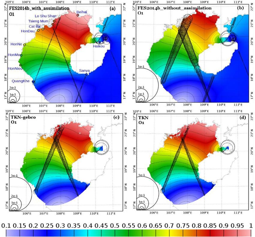
1584                                   V. Piton et al.: Sensitivity study on the main tidal constituents of the Gulf of Tonkin

play a key role in estuarine dynamics. Affecting mixing, in-        fice, Statistical Yearbook of Vietnam, 2017). This region is
fluencing a stronger or weaker stratification depending on the      also a key to the economy of Vietnam, with Ha Long Bay
sea water intrusion, and determining the characteristics of the     (a UNESCO world heritage site) for its particular touristic
water masses that can interact with the shelf circulation, tidal    value, and with the Hai Phong port system, connecting the
influence is often the main driver of the estuarine dynam-          north of the country to the world market. This latter is the
ics. Among other things, tidal asymmetry and density gradi-         second biggest harbor of Vietnam, with a particularly fast
ents are responsible for the presence of an estuarine turbid-       growth rate in terms of volume of cargo passing through the
ity maximum (mass of highly concentrated suspended sed-             port, of about 4.5 × 10⁶ to 36.3 × 10⁶ t from 1995 to 2016,
iments; Allen et al., 1980). Slack waters are found to favor        respectively (Statistical Yearbook of Vietnam, 2017). How-
sedimentation and deposition, while flood and ebb tend to           ever, the harbor of Hai Phong is currently affected by an in-
enhance erosion and resuspension within the estuary, and the        creasing siltation due to tidal pumping, related to changes
tidal asymmetry induces a tidal pumping (i.e., spring tides are     in water regulation by dams since the late 1980s. Such phe-
more energetic than neap tides). Understanding the dynamics         nomenon forces a dredging effort to be more and more im-
of these turbidity maxima is crucial for harbors and coastal        portant each year, with USD 6.6 million spent on dredging
maritime traffic management as they are often related to high       activity in 2013 (Lefebvre et al., 2012; Vietnam maritime
siltation rates, necessitating regular dredging by local author-    administration, 2017). In this particular case, fine-scale tidal
ities (Owens et al., 2005; Vinh et al., 2018). These zones of       modeling is of great interest for harbor management and risks
accumulation of suspended sediments are also important for          prevision.
the ecology of coastal areas as sediments can carry pollutants         The tides in the SCS and in the GoT have been extensively
that endanger water quality (Eyre and McConchie, 1993).             studied since the 1940s (Nguyen, 1969; Ye and Robinson,
The ability to understand and predict the formation of these        1983; Yu, 1984; Fang, 1986). Skimming through the litera-
zones related to tide cycles is therefore crucial for coastal and   ture, a lot of discrepancies exist in the cotidal charts before
local activities.                                                   the 1980s, especially over the shelf areas. With the develop-
   The Gulf of Tonkin (from hereafter GoT) covers an area           ment of numerical models, the discrepancies have been sig-
of 115 000 km2 from about 16◦ 100 to 21◦ 300 N and 105◦ 30          nificantly reduced by improving the accuracy of tides and
to 111◦ E. This crescent-shaped semi-enclosed basin, also re-       tidal currents prediction.
ferred as Vi.nh Bǎc Bô in Vietnam or as Beibu Gulf in China,          Wyrtki (1961) was the first to identify the main tidal con-
is 270 km wide and 500 km long and lies in between China to         stituents in the SCS (O1 , K1 , M2 , and S2 ), and Ye and Robin-
the north and east and Vietnam to the west. It is characterized     son (1983) were the first to successfully simulate the tides in
by shallow waters as deep as 90m and is open to the South           the area. Until recently, only a few numerical studies have
China Sea (SCS) through the south of the Gulf and to the east       focused on the GoT (Fang et al., 1999; Manh and Yanaki,
through the narrow Hainan Strait (Fig. 1a). This latter, also       2000; van Maren and Hoekstra, 2004) and on the Hainan
known as Qiongzhou Strait, is on average 30 km wide and             Strait (Chen et al., 2009). By using, for the first time, a high-
50 m deep and separates the Hainan Island from the Zhan-            resolution model (ROMS at 1/25◦ ) and a combination of all
jiang peninsula (Leizhou Peninsula, part of mainland China).        available data, Minh et al. (2014) gave an overview of the
The bottom topography in the GoT and around Hainan Island           dominant physical processes that characterize the tidal dy-
is rather complex, constantly changing, especially along the        namics of the GoT, by exploring its resonance spectrum. This
coastlines, and partly unknown. Furthermore, the Ha Long            study improved the existing state of the art in numerically re-
Bay area contains about 2000 islets, also known as notches,         producing the tides of the GoT; however it also showed the
sometimes no bigger than a few hundreds square meters.              limitations of using a 3D model to represent the tidal spec-
   The GoT is subjected to the Southeast Asian subtropical          trum. Indeed, large discrepancies between the model and ob-
monsoon climate (Wyrtki, 1961), and therefore largely in-           servations especially for the M2 harmonics and for the phase
fluenced by seasonal water discharges from the Red River            of S2 were found. The authors explained those discrepancies
(Vietnam) and by many smaller rivers such as the Qinjiang,          by the lack of resolution in the coastal areas due to limitations
Nanliu, and the Yingzai rivers (China). The Red River, which        implied by the use of a regular grid and a poorly resolved
brings in average 3500 m3 s−1 (Dang et al., 2010) of water          bathymetric dataset.
along 150 km of coastline, was ranked as the ninth river in the        The SCS and the GoT are some of the few regions
world in terms of sediment discharge in the 1970s with 145–         in the world where diurnal tides dominate the semidiur-
160 Mt yr−1 (Milliman and Meade, 1983). Its sediment sup-           nal tides (Fang, 1986). The tidal form factor (F ), or am-
ply was drastically reduced since then to around 40 Mt yr−1         plitude ratio, defined by the ratio of the amplitude of the
of sediment (Le et al., 2007; Vinh et al., 2014). The Red           two main diurnal over the semidiurnal constituents, as F =
River area accounts for the most populated region of the GoT,       (O1 + K1 )/(M2 + S2 ), provides a quantitative measure of the
with an estimated population of 21.13 million in 2016, cor-         general characteristics of the tidal oscillations at a specific
responding to an average population density of 994 inhab-           location. If 0 < F < 0.25, then the regime is semidiurnal,
itants per square kilometer (from the General Statistics Of-        if 0.25 < F < 1.5, the regime is mixed primarily semidiur-

Geosci. Model Dev., 13, 1583–1607, 2020                                               www.geosci-model-dev.net/13/1583/2020/
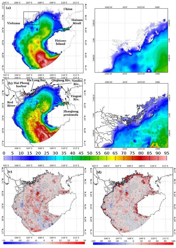
V. Piton et al.: Sensitivity study on the main tidal constituents of the Gulf of Tonkin                                          1585

Figure 1. (a, left) GEBCO bathymetry (in meters) and (a, right) details of the Ha Long Bay area (black rectangle in a, left). (b, left)
TONKIN_bathymetry dataset merged with TONKIN_shorelines over GoT and (b, right) zoomed in on the Ha Long Bay area. (c) Absolute
(in meters) and (d) relative (in percent) differences between TONKIN_bathymetry and GEBCO bathymetry (in meters).

nal, if 1.5 < F < 3, the regime is mixed primarily diurnal,           southwest is weak for the semidiurnal tides and strong for
and if F > 3, the regime is diurnal. Values of F shown in             the diurnal ones. A second branch of energy (also diurnal
Fig. 2 are calculated using tidal amplitudes from FES2014b-           tidal waves) enters the GoT through the Hainan Strait (Ding
with-assimilation (product described in Sect. 2.2.3). At the          et al., 2013).
entrance of the GoT and at the Hainan Strait, the tides are              In coastal seas and bays, tides are primarily driven by the
defined as mixed primarily diurnal, with F varying from 1.5           open ocean tide at the mouth of the bay. By resonance of
and 2.2 depending on the given locations. At the Red River            a constructive interference between the incoming tide and a
Delta, F is around 15, attesting to a diurnal regime. Indeed,         component reflected from the coast, a large tide amplitude
the major branch of energy flux entering the basin from the           can be generated. In the GoT case, tidal waves enter the

www.geosci-model-dev.net/13/1583/2020/                                                   Geosci. Model Dev., 13, 1583–1607, 2020
1586                                    V. Piton et al.: Sensitivity study on the main tidal constituents of the Gulf of Tonkin

                                                                     response of the tidal solutions to the calibration of the bottom
                                                                     friction and to the improvements in the bathymetry.
                                                                        As evidenced by Fontes et al. (2008) and Le Bars et
                                                                     al. (2010), local tidal simulations are mainly affected by the
                                                                     bathymetry and the bottom stress parametrization. These lat-
                                                                     ter often lack of details in remote coastal regions and/or in
                                                                     poorly sampled regions (in terms of bathymetry and tide
                                                                     gauges). It is particularly the case for the GoT. By its lo-
                                                                     cation at the boundary between China and Vietnam and
                                                                     by its intense maritime transport activity, the region is ex-
                                                                     tremely difficult to sample, in particular in the highly pro-
                                                                     tected region of Ha Long Bay, in the Hainan Strait, and in
                                                                     the nearshore/coastal areas. In situ data and soundings are
                                                                     consequently rare and yet extremely valuable. The precise
                                                                     goal of the present study is therefore to build an improved
Figure 2. Map of tidal form factor F computed with the amplitudes
of tidal waves O1 , K1 , M2 , and S2 obtained from FES2014b-with-    bathymetry and coastline database over the GoT and to de-
assimilation. The range 0 < F < 0.25 corresponds to semidiurnal      fine the best configuration for bottom stress parameterization
regime, 0.25 < F < 1.5 corresponds to mixed primarily semidiur-      in this region, evaluating the impact of those parameters on
nal, 1.5 < F < 3 corresponds to mixed primarily diurnal, and F > 3   the tidal representation in the GoT. The resulting optimized
corresponds to diurnal regime.                                       configuration will then be used for future numerical studies
                                                                     of ocean dynamics and sediment transport in the region. For
                                                                     that, we first worked on the improvement in the general and
                                                                     global bathymetric datasets available, i.e., GEBCO (Mon-
basin from the adjacent SCS, and due to the basin geome-             ahan, 2008), the Smith and Sandwell bathymetry (Smith
try, O1 and K1 resonate (Fang et al., 1999). Their amplitudes        and Sandwell, 1997), and the ETOPO1 Global Relief Model
reach 90 and 80 cm respectively. The Coriolis force deflects         (Amante and Eakins, 2009), by incorporating new sources
the incoming waves to the right and pushes them against the          of data. We then worked on the optimization of the bottom
northern enclosure of the basin. Once the waves are reflected,       stress parameterization. Our approach to addressing the is-
they propagate southward until they slowly dissipate by fric-        sue of the parametrization and to evaluating the impact of
tion. Fang (1999) found that the amplitude of the tide grad-         our configuration setup is based on the use of the hydro-
ually decreases from 4 to 2 m north to south during spring           dynamical model T-UGOm model of Lyard et al. (2006).
tide. The amplitude of O1 in the GoT is larger than K1 be-           Thanks to its frequency-domain solver, shortly described in
cause of a larger resonance effect, even though its amplitude        the next sections, T-UGOm can indeed perform tidal simula-
in the SCS is smaller than K1 (Minh et al., 2014). The largest       tions at an extremely limited computational cost (compared
semidiurnal waves of the GoT are M2 and S2 . They both ap-           to time-stepping solver), in our case roughly 80 times faster
pear as a degenerated amphidrome with smallest amplitudes            than usual time-stepping hydrodynamical models (i.e., from
near the Red River Delta in the northwestern head of the Gulf        a few minutes for T-UGOm compared with hours/days). Fur-
(between 5 and 15 cm for M2 and below 5 cm for S2 ) (Hu              thermore, different formulations for the bottom friction can
et al., 2001). Given those values of amplitude, Van Maren            be prescribed along with a varying spatial distribution of its
et al. (2004) defined the tidal regime in the GoT as mesoti-         related parameters (roughness or friction factor). These par-
dal and locally even macrotidal, even though diurnal tidal           ticular assets allow a large number of sensitivity tests to be
regimes are usually mainly microtidal.                               performed at a reasonable computational cost on bathymet-
   Our first objective in this paper is to propose a robust and      ric and bottom stress parametrization, hence speeding up the
simple approach that allows the quantification of the sensi-         processes of precise tuning and calibration/validation of our
tivity of the tidal solutions to bottom friction parameteriza-       configuration.
tion and to bathymetric changes in the Gulf of Tonkin. This             In Sect. 2, we describe the bathymetry, shorelines and wa-
article furthermore represents the first step in a more com-         terways construction as well as the numerical model and the
prehensive modeling study aiming at representing the trans-          modeling strategy in terms of sensitivity experiments. The
port and the fate of sediments from the Red River to the             data used for model evaluation and the metrics used for this
Gulf of Tonkin using the tridimensional structured coupled           evaluation are also presented in this section. In Sect. 3 we
SYMPHONIE–MUSTANG model (Marsaleix et al., 2008;                     present the results regarding the sensitivity of simulations
Le Hir et al., 2011). In this framework, our final objective is      to bottom stress parametrization and to bathymetry. Conclu-
to optimize the configuration (bathymetry) and parameteri-           sions and outlook are given in Sect. 4.
zation (bottom stress) that will be used in this forthcoming
study. These objectives are based on the quantification of the

Geosci. Model Dev., 13, 1583–1607, 2020                                                www.geosci-model-dev.net/13/1583/2020/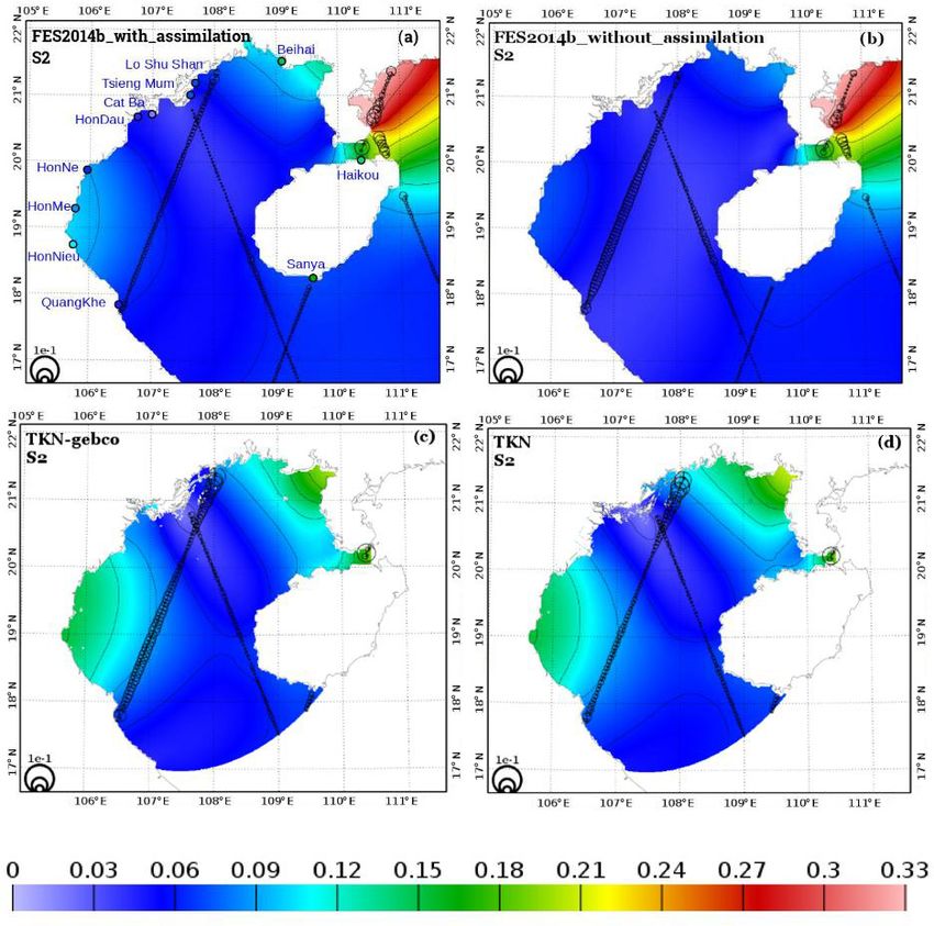
V. Piton et al.: Sensitivity study on the main tidal constituents of the Gulf of Tonkin                                     1587

Figure 3. Shoreline products from OpenStreetMap (blue line), GSHHG (yellow line), and TONKIN_shorelines (red line) superimposed on
a satellite image downloaded from Bing (© Bing™) over a small region of the GoT.

2     Methods and tools                                            lected before accurate GPS measurements in the area. Our
                                                                   objective in this study is to propose a grid matching the re-
2.1    Shorelines and bathymetry construction                      ality (i.e., Bing maps, our reference) as close as possible;
                                                                   therefore, none of these databases looked precise enough to
                                                                   meet our expectations. Consequently, we have built our own
The first step of our work is to improve the shoreline             shorelines dataset, named TONKIN_shorelines, by using the
and bathymetry precision. Two global digital shorelines are        POC Viewer and Processing (POCViP) software (available
commonly used for representing the general characteris-            on the CNRS sharing website, https://mycore.core-cloud.net/
tics of the GoT shorelines: the Global Self-consistent, Hi-        index.php/s/ysqfIlcX5njfAYD/download, last access: 9 De-
erarchical, High-resolution Geography Database (GSHHG,             cember 2019), developed at LEGOS. The satellite and aerial
Wessel and Smith, 1996) and the free downloadable maps             images of the region, previously downloaded from Bing,
from OpenStreetMap (OpenStreetMap contributors, 2015;              are georeferenced with POCViP. The software allows the
retrieved from http://www.planet.openstreetmap.org, last ac-       user to draw nodes and segments with a resolution as fine
cess: 20 May 2018). The GSHHG and OpenStreetMap shore-             as needed. The resulting TONKIN_shorelines database has
line products are both superimposed on satellite and aerial        a resolution down to 10 m, and its accuracy is observable
images of the GoT downloaded from Bing (https://www.               in Fig. 3. We followed the same procedure for building a
bing.com/maps, last access: 15 June 2018) and used now             waterways database of the Red River system. This latter is
as our reference. Bing is chosen here for the accessibility        also included in TONKIN_shorelines. For the Ha Long Bay
of its open data, which makes our shoreline construction           area, another strategy has been considered since drawing
method doable by everyone. Figure 3 shows the shoreline            by hand each islet would have been unaffordably time con-
products superimposed on a downloaded image of a small             suming. In this case, images from the Shuttle Radar Topog-
region of the GoT. When closely comparing the shoreline            raphy Mission (SRTM) (https://earthexplorer.usgs.gov/, last
products to the images, it appears that the OpenStreetMap          access: 2 July 2018) were downloaded and coastlines got ex-
product looks fairly reasonable all along the coastlines of the    tracted and merged with TONKIN_shorelines.
GoT, except in the Ha Long Bay area (not shown) where                 Because of the shallowness of the area, the bathymetry
the complex topography and the islets are clearly too nu-          of the GoT is a critical point and could have a strong
merous. However, the OpenStreetMap shoreline is most of            impact on tidal simulations as it is often the main con-
the time shifted by a few meters westwards compared to             straint in tidal propagation (Fontes et al., 2008). The
the land (Fig. 3). The GSHHG dataset suffers from the              GEBCO 2014 (30 arcsec interval grid) dataset is largely
same problem but shifted by up to 500 m eastwards. The             based on a database of ship-track soundings, whose res-
observed shifts in both OpenStreetMap and GSHHG prod-              olution can be locally much finer than 1 km, but gridded
ucts are not documented but could be due, among other              data are provided with a ∼ 1 km resolution (as explained
things, to the use of nautical charts and/or local topography      on the GEBCO website: https://www.gebco.net/data_and_
maps for product construction, which could have been col-

www.geosci-model-dev.net/13/1583/2020/                                               Geosci. Model Dev., 13, 1583–1607, 2020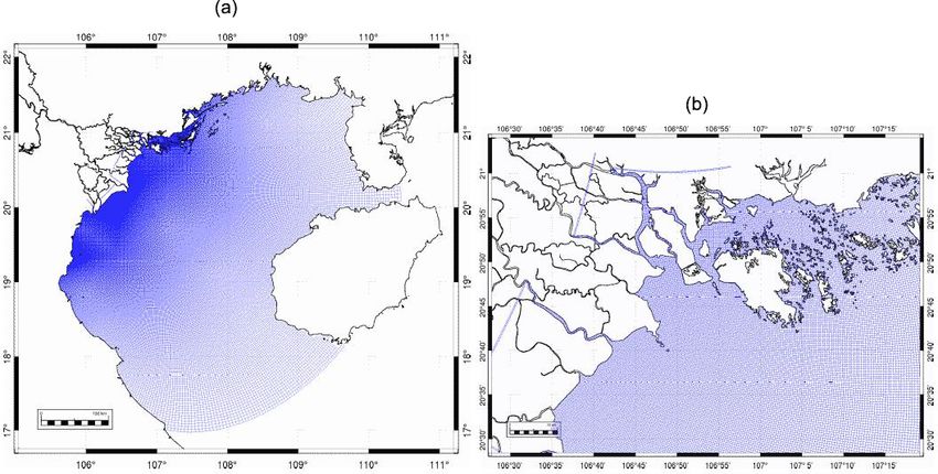
1588                                  V. Piton et al.: Sensitivity study on the main tidal constituents of the Gulf of Tonkin

products/historical_data_sets/ (last access: 16 Novem-            2.2     Model, configuration and forcings
ber 2019). The GEBCO dataset can hence be used to rep-
resent the slope and the shape of the basin at a relatively       2.2.1    T-UGOm hydrodynamic model
large scale (Fig. 1a, b). However, this 1 km resolution is too
low to accurately represent detailed geomorphological fea-        The tidal simulations are based on the unstructured grid
tures, in particular in coastal regions, near the delta, and in   model T-UGOm (Toulouse Unstructured Grid Ocean Model)
the Ha Long Bay area. For the purpose of providing an im-         developed at LEGOS and is the follow-up of MOG2D (Car-
proved tidal solution, we have developed a bathymetry with        rère and Lyard, 2003). In its standard applications, T-UGOm
a better precision, named TONKIN_bathymetry (Fig. 1c, d).         uses unstructured triangle meshes allowing for an optimal
For that, we have merged the GEBCO bathymetry with dig-           grid resolution flexibility, in particular to discretize com-
italized nautical charts of type CM-93 via OpenCPN (https:        plex coastal geometry regions, to follow various local dy-
//opencpn.org/, last access: 20 July 2018). Note that bathy-      namical constraints, such as rapid topography changes, or to
metric data from nautical charts in coastal shallow areas are     simply adapt resolution in regions of special interest. The
often chosen to be shallower than the real bathymetry for         flexibility of unstructured triangle meshes is fully adequate
navigation security purposes. We also incorporated the tidal      for fine-scale modeling, especially in delta or estuarine sys-
flats digital elevation model from Tong (2016). This author       tems, whereas usual structured meshes may struggle to rep-
used waterlines from Landsat images of 2014 to construct          resent fine geography of certain areas. The T-UGOm model
a surface model from elevation contours. As tidal flats are       is widely used in global to coastal modeling, mostly for
suffering from a tidal regime with submersion during flood        tidal simulations; in the representation of semi- and quarter-
tide and exposure during ebb tide, their representation is cru-   diurnal barotropic tides in the Bay of Biscay (Pairaud et
cial in tidal modeling. TONKIN_bathymetry is merged with          al., 2008), in studying the tidal dynamics of the macro-tidal
TONKIN_shorelines dataset.                                        Amazon estuary (Le Bars et al., 2010), in the representation
   This scattered bathymetric dataset shows realistic small-      of tidal currents over the Australian shelves (Cancet et al.,
scale structures and depths over the shelf and in the Ha Long     2017), and in assessing the role of the tidal boundary con-
Bay area. The details and the islets of the bay are now rep-      ditions in a 3D model in the Bay of Biscay (Toublanc et
resented (Fig. 1c, d), as well as the Red River waterways. In     al., 2018). Furthermore, T-UGOm has proven its accuracy in
the deeper part of the basin, near the boundary, two deeper       global barotropic tidal modeling in the Corsica Channel (Vi-
branches (in light red) are distinguishable. These latter could   gnudelli et al., 2005) and in a global assessment of different
correspond to the location of the ancient river bed of the Red    ocean tide models (Stammer et al., 2014).
River during the last glacial time, which split in two around        In addition to its traditional time-stepping solver, it
18◦ N–108◦ E (Wetzel et al., 2017). The biggest differences       has the remarkable particularity to include a frequency-
compared to GEBCO are observed in the central part of the         domain solver kernel, which solves for the 2D/3D quasi-
region and in the Hainan Strait (Fig. 1e, f). In the strait,      linearized tidal equations. This spectral mode solves the
the GEBCO bathymetry underestimates depths by roughly             quasi-linearized Navier–Stokes equations in the spectral do-
20 m (∼ 50 % in terms of relative difference) compared to         main, in a wave by wave, iterative process (to take into
TONKIN_bathymetry. In the center, differences can be up to        account nonlinear effects such as bottom friction). It has
30 m between the two datasets (not shown on the color bar),       demonstrated its efficiency (accuracy and computational
corresponding to relative differences of up to 100 %. Such        cost) for the astronomical tide simulation as well as for the
high observed discrepancies are due to the interpolation of       nonlinear tides. The frequency-domain solver can be used ei-
the scattered measuring points from the nautical charts. High     ther on triangle or quadrangle unstructured mesh and there-
relative differences are also observed all along the coast-       fore can be used on any C-grid configuration. Compared to
lines, corresponding for most of them to the integration of       a traditional time-stepping mode that simulates the temporal
the intertidal dynamical elevation model (DEM) in the Red         evolution of the tidal constituents over a given period, the nu-
River Delta area, as well as to a better resolution in shal-      merical cost of the frequency-domain mode (2D) is roughly
low areas obtained from the nautical charts. Discrepancies        1000 times smaller.
in most other parts of the basin remain roughly below 30 %.          For our purpose of assessing the sensitivity to various pa-
Patches of differences of about 40 % between the datasets         rameters of the tide representation by the model, T-UGOm
are also observed at the open ocean boundary of the domain,       is set up in a 2D barotropic, quadrangle grid, shallow-water,
with GEBCO also underestimating depths in the southern-           and frequency-domain mode (version of the code: 4.1 2616).
most part.                                                        This configuration (including TONKIN_bathymetry and the
   We draw attention to the fact that the                         specific version of T-UGOm code) is from hereafter named
TONKIN_bathymetry dataset provides an improvement                 TKN. The main advantage of this fast and reduced-cost
to the available bathymetric dataset but that some flaws and      solver is the possibility to perform in an affordable time a
uncertainties still exist, partly due to sampling methods and     wide range of experiments at the regional or global scale,
shallower waters induced by nautical charts data.                 in order to parameterize the model, such as the following:

Geosci. Model Dev., 13, 1583–1607, 2020                                             www.geosci-model-dev.net/13/1583/2020/
V. Piton et al.: Sensitivity study on the main tidal constituents of the Gulf of Tonkin                                        1589

Figure 4. Model mesh over (a) the GoT and (b) zoomed in on the Ha Long Bay region. The maximum refinement (150 m) is reached in the
river channels.

optimize bottom stress parametrization, test bathymetry im-         which produces a bipolar grid. The singularities associated
provements, and other numerical developments. In our case,          with the two poles are located in the continental mask,
the run duration of a spectral simulation with T-UGOm lasts         slightly to the north of the numerical domain, where the hor-
on average 6 min (CPU time), which is roughly 40 times              izontal resolution is the strongest (Fig. 4). This first guess is
quicker than a simulation with a regional circulation model         then slightly modified to control the extension of the grid off-
such as SYMPHONIE (Marsaleix et al., 2008; CPU time is              shore, in practice to prevent extension beyond the continen-
approximately 4 h for a 9-month simulation, corresponding           tal shelf. As in Madec and Imbard (1996) this second stage
to the required time with SYMPHONIE to separate the tidal           is partly numerical (and preserves the orthogonality of the
waves).                                                             axes of the grid). The largest edges of the quadrangles are
   Another useful functionality of T-UGOm for our study is          about 5 km at the boundaries of the domain and the smallest
the possibility to locally prescribe the bottom friction, includ-   are about 150 m long, with a maximum refinement located
ing the roughness length and also the choice of parametriza-        in the river channels (Fig. 5). This grid allows the complex-
tion type. In some shallow coastal regions like the GoT, the        ity of the islets of Ha Long Bay as well as the details of the
presence of fluid mud flow and fine sediments can induce            coastlines of the Red River Delta to be represented. A regular
dramatic changes on bottom friction. The quadratic parame-          C-grid would hardly take into account such complex topog-
terization may be obsolete, and a linear parameterization may       raphy and details.
be more adequate (Le Bars et al., 2010) and will be tested
hereafter. This functionality is essential in those particular      2.2.3   Tidal open-boundary conditions
regions like shallow estuaries, where the influence of bottom
friction on the tides propagation is crucial.                       For modeling barotropic tidal waves, nine tidal constituents
                                                                    have been imposed as open boundary conditions (OBCs)
2.2.2   Numerical domain over the GoT                               in elevation (amplitude and phase) for our domain: O1 , K1 ,
                                                                    M2 , S2 , N2 , K2 , P1 , Q1 , and M4 . Since the astronomical
The numerical domain over the GoT, built from the                   spectrum of tide is dominant in the GoT, eight out of the
TONKIN_bathymetry, is discretized on an unstructured grid           nine constituents simulated are astronomical constituents,
made of quadrangle elements (Fig. 3). The most com-                 and M4 is chosen here as a representative of all nonlinear
monly used elements in T-UGOm are triangles; however                interactions. These constituents, ordered by their amplitudes
here the final goal of our work is to use the resulting grid        (in the GoT), are the main tidal waves in the GoT and
for coupled hydrodynamical–sediment transport models like           come from the FES2014b global tidal model resolved on
SYMPHONIE–MUSTANG using quadrangle structured C-                    unstructured meshes but distributed on a resolution-coherent
grids. We therefore run the T-UGOm tidal solver on a quad-          1/16◦ × 1/16◦ grid. FES2014b (Carrère et al., 2016) is the
rangle grid. As in Madec and Imbard (1996), this grid is            most recent available version of the FES (finite element
semi-analytical. A first guess is provided by the analytical re-    solution) global tide model that follows the FES2012
versible coordinate transformation of Bentsen et al. (1999),        version (Carrère et al., 2012). The FES2014b global tidal

www.geosci-model-dev.net/13/1583/2020/                                                Geosci. Model Dev., 13, 1583–1607, 2020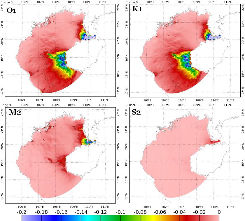
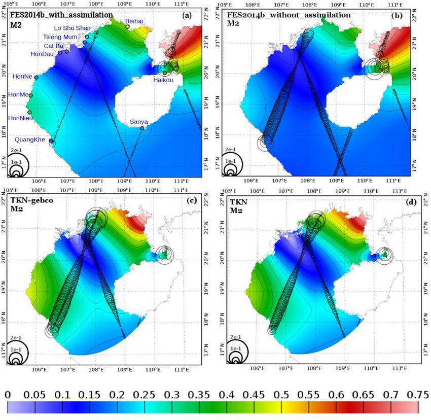
1590                                    V. Piton et al.: Sensitivity study on the main tidal constituents of the Gulf of Tonkin

Figure 5. O1 tidal amplitude (in meters) from different products: (a) FES2014b-with-assimilation, (b) FES2014b-without-assimilation,
(c) TKN-gebco, and (d) TKN. The circle diameter is proportional to the complex error (Appendix; Eq. A2) between the solutions and
satellite altimetry (in meters). The colored circles denote the amplitude of O1 harmonic measured at the corresponding tide gauge station.

atlas includes 34 tidal constituents and is based on the               of the prior FES2014b-without-assimilation solutions and
resolution of the tidal barotropic equations with T-UGOm               the subsequent higher efficiency of data assimilation, this
(frequency-domain solver for the astronomical tides and                latest FES2014b-with-assimilation version of the FES2014
time-stepping solver for the nonlinear tides, described in             atlas has reached an unprecedented level of precision and
the above section). The FES2014b bathymetry has been                   has shown accuracy that is superior to any other previ-
constructed from the best available (compared to previous              ous versions (see http://www.aviso.altimetry.fr/en/data/
FES versions) global and regional DTMs (dynamical                      products/auxiliary-products/global-tide-fes.html, last ac-
topography models) and corrected from available depths                 cess 15 June 2018; Florent Lyard, personal communication,
soundings (nautical charts, ship soundings, and multibeam              10 October 2018).
data) to get the best possible accuracy, typically 1.3 cm                 The tidal distribution of the O1 , K1 , M2 , and S2 tidal waves
RMS (root-mean-square error) for the M2 constituent in the             and their first harmonics from FES2014b-with-assimilation
deep ocean before data assimilation. The tidal simulation              and FES2014b-without-assimilation is shown in Figs. 4a, b,
performed using this configuration and without assimilation            5a, b, 6a, b, 7a, and b, as well as their error along the satellite
is called FES2014b-without-assimilation. Moreover, in ad-              altimetry track dataset of CTOH-LEGOS (described below in
dition to the hydrodynamic solutions, data-derived altimetry           Sect. 2.3.1). FES2014b-with-assimilation shows negligible
and tide gauges harmonic constants have been assimilated,              errors compared to FES2014b-without-assimilation thanks
using a hybrid ensemble/representer approach, to improve               to the assimilation. The main interest of using FES2014b-
the atlas accuracy for 15 major constituents and fulfill               without-assimilation in our study is to assess the real ca-
the accuracy requirements in satellite ocean topography                pacity of the FES model to reproduce the tidal harmonics
correction. This version of FES will from hereafter be named           without using data assimilation, whereas FES2014b-with-
FES2014b-with-assimilation in the following, in comparison             assimilation can be used together with satellite altimetry as a
to FES2014b-without-assimilation. Thanks to the accuracy               reference to evaluate tidal solution errors.

Geosci. Model Dev., 13, 1583–1607, 2020                                                   www.geosci-model-dev.net/13/1583/2020/
V. Piton et al.: Sensitivity study on the main tidal constituents of the Gulf of Tonkin 1591
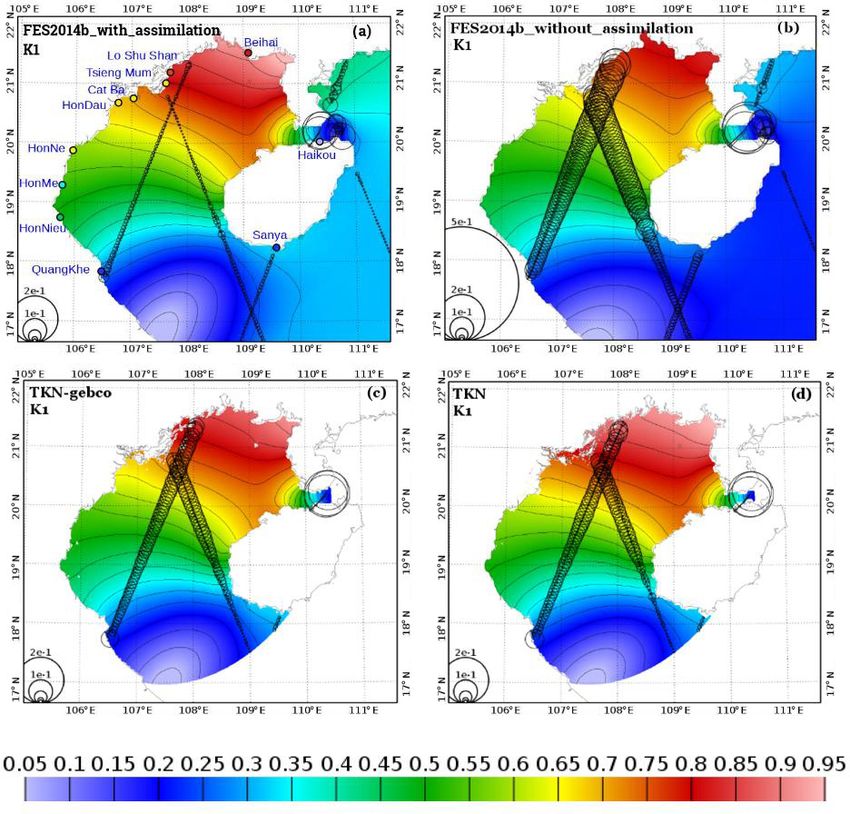
Figure 6. Same as Fig. 5 for K1 .
The T-UGOm code, the model grid, and the configuration tom stress is significant. The bottom stress is thus a cru-
files used for our simulations are available in Zenodo/Piton cial component for modeling nearshore circulation and sedi-
(2019a–c; see Code and data availability section). ment transport dynamics (Gabioux et al., 2005; Fontes et al.,
2008). The bottom stress formulation depends upon a nondi-
2.3 Simulations and evaluation mensional bottom drag coefficient (or friction coefficient) CD
and can be obtained, in barotropic mode, as follows:
We use the model configuration described above to assess the
impact of the improvement in our bathymetry database and to τb = ρCD |u|u, (1)
optimize the representation of bottom friction in the model.
For that we perform sensitivity simulations that we compare with u the depth averaged velocity and ρ the fluid density.
with available data using specific metrics. Those tools and In this study, we test two commonly used parameteriza-
methods are presented in this section. tions: a constant drag coefficient CD assuming a constant
speed profile and a drag coefficient CD depending upon the
2.3.1 Modeling strategy and sensitivity experiments roughness height z0 .
In the first parameterization, a constant profile of the
The T-UGOm 2D model (in its frequency-domain, itera-
speed is assumed over the whole water height, leading to
tive mode) is run on the high-resolution grid described in
quadratic bottom stress and a constant CD that depends on
Sect. 2.2.2. The following sections describe the tests per-
the Chézy coefficient C and on the acceleration due to grav-
formed for the bottom friction parametrization.
ity g (Dronkers, 1964) as follows:
Bottom stress parametrization g
CD = . (2)
C2
In shallow areas where current intensities are strong due to a
macro-tidal environment combined with strong rivers flows In the second parameterization, a logarithmic profile of the
and winds forcing, the sensitivity of the model to the bot- speed is assumed over the whole water column (Soulsby et
www.geosci-model-dev.net/13/1583/2020/ Geosci. Model Dev., 13, 1583–1607, 2020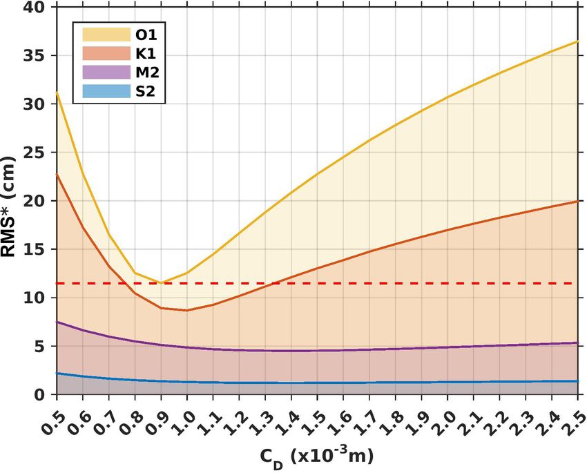
1592                                  V. Piton et al.: Sensitivity study on the main tidal constituents of the Gulf of Tonkin

Figure 7. Same as Fig. 5 for M2 .

al., 1993), leading to a CD depending upon the roughness          correspond to the friction coefficient resolution in 3D mod-
length z0 , the total water height H , and the von Kármán’s       els.
constant κ = 0.4 as follows:                                         In the case of fluid mud when the bottom friction is
                             !2                                   purely viscous and the velocity profiles are linear, Gabioux
            κ (H − z0 )                                           et al. (2005) described the τb as follows:
CD =                              .                        (3)
         H ln zH0 + z0 − H                                        τb = ρru,                                                   (4)
The roughness length z0 (also called roughness height) de-        with r corresponding here to the friction coefficient.
pends on not only the morphology of the bed (i.e., the pres-         A third parameterization of the coefficient of friction is
ence of wavelets or not) but also the nature of the bottom sed-   tested in this study; a linear profile of the speed is assumed
iment. In presence of fluid mud, the friction is considered as    over the whole water column, which characterizes viscous
purely viscous (Gabioux, 2005). However, the repartitioning       conditions. In this case, a linear bottom stress is assumed,
of sediments and the structure of the seabed are not uniform      and r depends on the frequency of the forcing wave ω (here
over the GoT shelf as the Red River discharge causes patches      O1 ) and the fluid kinematic viscosity v as follows:
of sediments of different natures (Natural Conditions and En-          √
vironment of Vietnam Sea and Adjacent Area Atlas, 2007).          r = ωv.                                                     (5)
Consequently, we can expect z0 to vary spatially. This issue
can be addressed with T-UGOm since it contains a domain           In this study, these three formulations of the coefficient of
partition algorithm allowing it to take into account the spa-     friction (Eqs. 2, 3, and 5) are tested for model parameteriza-
tial variability in the seabed roughness. Furthermore, this CD    tion, varying, respectively, the value of CD , the value of z0 ,
parameterization, which includes a logarithmic profile of the     and the value of r.
speed, allows the adaption of CD to the model vertical reso-
lution by considering the water column depths, as a way to

Geosci. Model Dev., 13, 1583–1607, 2020                                             www.geosci-model-dev.net/13/1583/2020/
V. Piton et al.: Sensitivity study on the main tidal constituents of the Gulf of Tonkin 1593
Figure 8. Same as Fig. 5 for S2 .
Sensitivity to uniform friction parameters in the seafloor morphology is not fully taken into considera-
tion. To take this variability into account, the spatial variabil-
Sensitivity numerical experiments were first conducted in or- ity in the seabed roughness must be prescribed to the model.
der to assess the sensitivity of the model to uniform param- For that, our study area is divided into several zones based on
eters of friction for two of the parameterizations described seabed sediment types repartition obtained from the Natural
above, which include a quadratic bottom stress with a uni- Conditions and Environment of Vietnam Sea and Adjacent
form drag coefficient CD (i.e., CD = constant) (Eqs. 1 and 2) Area Atlas (2007).
and a logarithmic variation in CD depending on a uniform The third set of sensitivity experiments (SET3, Tests A to
bottom roughness height z0 , i.e., CD = f (z0 , H ) (Eq. 3). For E in Table 1) consisted of prescribing a linear velocity profile
that, we performed a first set (SET1) of 45 tests, running the only in the area of fine mud, following Eqs. (4) and (5), with
model with a constant CD with CD values spanning from a fixed r = 1.18 × 10⁻⁴ m (see Fig. 10a), and testing differ-
0.5 × 10⁻³ to 5.0 × 10⁻³ m (see Fig. 9 where we plotted ent values of uniform z0 (from 1.0 × 10⁻² to 1.0 × 10⁻⁶ m)
CD values spanning from 0.5 to 2.5 × 10⁻³ m). We then per- over the rest of the region, prescribing a logarithmic velocity
formed a second set (SET2) of six tests running the model profile. This value of r is taken from the value empirically
with a CD = f (z0 , H ) by testing values from 1.0 × 10⁻¹ to tuned on the region of the Amazon estuary and shelf with the
1.0 × 10⁻⁶ m for z0 (see Fig. 10). configuration described in Le Bars et al. (2010).
The fourth set of sensitivity experiments (SET4, Tests 1 to
Sensitivity to the regionalization of the roughness 7 in Table 1) consisted of dividing the region into three zones,
coefficient according to a supposed spatial distribution of the seabed
sediments, inspired from the above-mentioned Vietnamese
As mentioned in the previous section, a uniform roughness atlas (Fig. 12b), as follows: zone 1 is mostly composed of
coefficient does not usually allow for reaching a satisfying muddy sand, zone 2 is composed of mud, and zone 3 is com-
level of accuracy over the whole domain, since the variability
www.geosci-model-dev.net/13/1583/2020/ Geosci. Model Dev., 13, 1583–1607, 20201594 V. Piton et al.: Sensitivity study on the main tidal constituents of the Gulf of Tonkin
Table 1. Description of SET3 and SET4 (in meters).
SET3 A B C D E F
Mud region (r) 1.18 ×10⁻⁴ 1.18 ×10⁻⁴ 1.18 ×10⁻⁴ 1.18 ×10⁻⁴ 1.18 ×10⁻⁴ 1.18 ×10⁻⁴
z0 in the rest 1.0 ×10⁻⁶ 1.0 ×10⁻⁵ 1.5 ×10⁻⁵ 1.0 ×10⁻⁴ 1.0 ×10⁻³ 1.0 ×10⁻²
of the domain
SET4 1 2 3 4 5 6 7
Region 1 (z0 ) 1.0 ×10⁻² 1.0 ×10⁻³ 1.0 ×10⁻⁴ 1.0 ×10⁻⁴ 1.0 ×10⁻⁴ 1.5 ×10⁻⁵ 1.5 ×10⁻⁵
Region 2 (z0 ) 1.5 ×10⁻⁵ 1.5 ×10⁻⁵ 1.5 ×10⁻⁵ 1.5 ×10⁻⁵ 1.0 ×10⁻⁴ 1.5 ×10⁻⁵ 1.5 ×10⁻⁵
Region 3 (z0 ) 1.0 ×10⁻⁴ 1.0 ×10⁻⁴ 1.0 ×10⁻⁴ 1.5 ×10⁻⁵ 1.5 ×10⁻⁵ 1.0 ×10⁻⁴ 1.0 ×10⁻³
posed of sand and coarser aggregates. In each zone, a value and position of these stations are shown in Fig. 5a. Ampli-
of z0 (from 1.0 × 10⁻² to 1.0 × 10⁻⁵ m) is prescribed follow- tudes and phases of O1 , K1 , M2 , and S2 at the 11 gauge sta-
ing a CD = f (z0 , H ) (Eq. 3). Note that for this set of exper- tions are available in Chen et al. (2009).
iments every combination of z0 was tested, yet for the sake
of clarity we show and describe in Sect. 4 only the ones with 2.3.3 Metrics
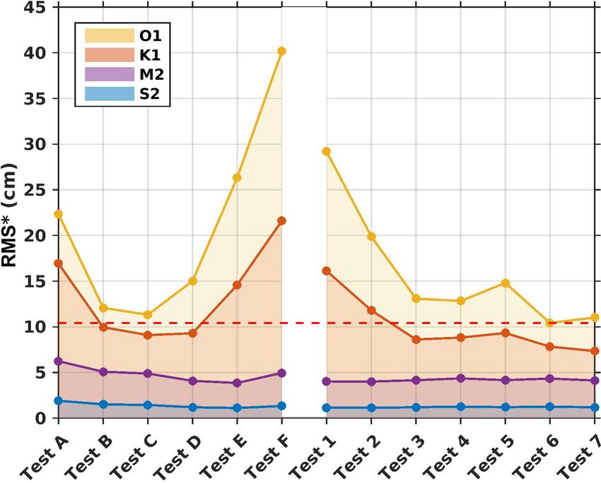
errors (see Sect. 2.3.3) for S2 solutions below 2.5 cm.
The fifth and last set of experiments (SET5) consisted of For comparison of the simulations with the tidal harmonics
dividing the domain into 12 zones, in order to refine the rep- from satellite altimetry, two statistical parameters (metrics)
resentation of the spatial distribution of the sediments of the are used. These are the root-mean-square error (RMS∗ ) and
seafloor following the Vietnamese atlas (Fig. 12c). Zones 1 the mean absolute error (MAE). The RMS∗ computation is
and 11 correspond to muddy sand, zones 2, 6, 10, and 12 based on a vectorial difference, which combines both ampli-
correspond to slightly gravelly sand, zones 3 and 5 corre- tude error and phase error into a single error measure. The
spond to sandy mud, zone 4 corresponds to fine mud, zone 7 errors computations are detailed in the Appendix.
corresponds to sandy gravel, zone 8 corresponds to slightly
gravelly mud, and zone 9 corresponds to sand. Different 3 Results
z0 values (varying from 1.0 × 10⁻² to 1.5 × 10⁻⁵ m), using
CD = f (z0 , H ), were prescribed to each of the 12 zones, and In this section we present the results concerning the sensitiv-
the corresponding runs were performed, each time imposing ity of the modeled tidal solutions to the choice of bathymetry
a random and different value to each zone. dataset and to the choice of bottom friction parameterization.
Spatially varying uniform friction parameters only slightly
2.3.2 Satellite data and tide gauges data for model improve the tidal solutions compared to uniform parameters.
assessment Furthermore, prescribing a linear parameterization in sup-
posed fluid mud areas does not allow a significant improve-
ment in the solutions, unlike in Le Bars et al. (2010). Lastly,
The evaluation of the performance of the simulations is
the reconstructed bathymetry dataset allows the semidiurnal
made with along-track tidal harmonics obtained from a 19-
tidal solutions to be strongly improved. The improvements
year-long (1993–2011) time series of satellite altimetry data
consist mainly of a correction near the coasts and of reduc-
available every 10 d from TOPEX/Poseidon (T/P), Jason-
ing the errors in phase (as can be expected from a bathymetry
1, and Jason-2 missions (https://doi.org/10.6096/CTOH_X-
upgrade). We present the results of the conducted sensitivity
TRACK_Tidal_2018_01). These data are provided by the
experiments in detail in the following subsections.
CTOH-LEGOS (Birol et al., 2016). The tracks of the al-
timeters passing over the GoT are shown in Figs. 5–8 and 3.1 Model sensitivity to bottom stress parameterization
are spaced by approximately 280 km. To complement those
data in the inter-track domain, we also compare our simu- 3.1.1 Sensitivity to a constant or varying CD (SET1 and
lations with the FES2014b-with-assimilation tidal atlas, as SET2)
explained in Sect. 2.2.3.
Harmonic tidal constituents at 11 tide gauge stations are We first analyze in this section and in the next one the sen-
also used for evaluation of the simulations. The data are sitivity to the parameterization of bottom friction. Firstly, to
distributed by the International Hydrographic Organization show the sensitivity to the choice of uniform friction parame-
(https://www.iho.int/, last access: 2 November 2019) and are ters, the model errors (Appendix; Eq. A2) compared to satel-
available upon request at https://www.admiralty.co.uk/ukho/ lite altimetry are shown in Fig. 9 (SET1) and Fig. 10 (SET2),
tidal-harmonics (last access: 2 November 2019). The name for the main tidal constituents (O1 , K1 , M2 , and S2 ) for each
Geosci. Model Dev., 13, 1583–1607, 2020 www.geosci-model-dev.net/13/1583/2020/V. Piton et al.: Sensitivity study on the main tidal constituents of the Gulf of Tonkin 1595
.
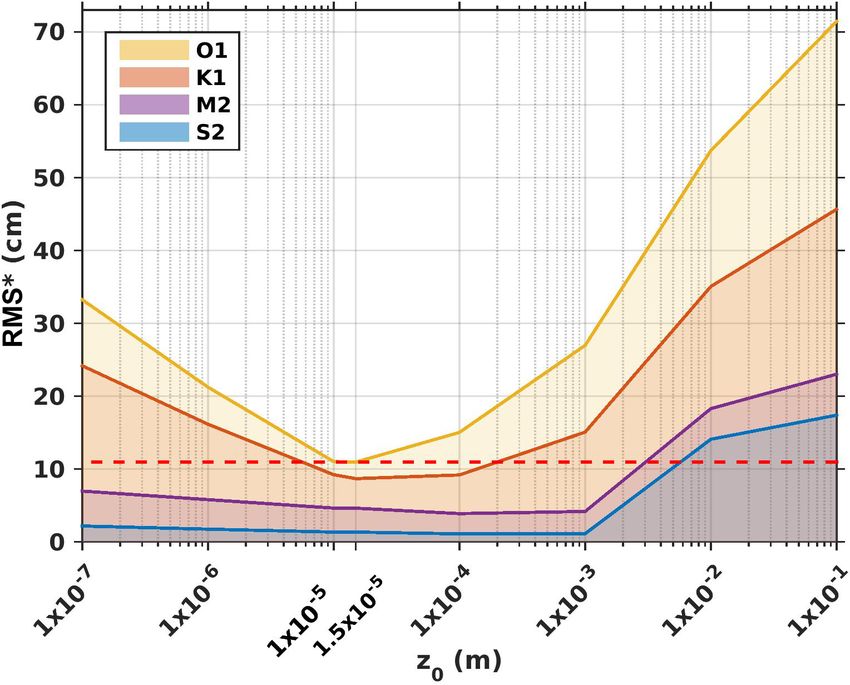
Figure 9. Model complex errors (Appendix; Eq. A2) relative to al- Figure 10. Model complex errors (Appendix; Eq. A2) relative to al-
timetry along-track data for tests performed with varying the val- timetry data for tests performed with varying the values of the uni-
ues of the uniform drag coefficient CD over the domain (SET1). form z0 over the domain (SET2). The space in between two lines
The space in between two lines corresponds to the error for each corresponds to the error for each wave. The yellow line corresponds
wave. The yellow line therefore corresponds to the cumulative er- to the cumulative errors for all four waves. The dashed red line cor-
ror for all four waves. The dashed red line corresponds to the responds to the smallest cumulative error, here equal to 10.96 cm
smallest cumulative error, here equal to 11.50 cm and obtained for and obtained for z0 = 1.5 × 10⁻⁵ m.
CD = 0.9 × 10⁻³ m
used in the GoT by Nguyen et al. (2014) of 1.0 × 10⁻³ m.
value of uniform CD and z0 tested in SET1 and SET2, de- The tests of sensitivity to the roughness length z0 show that
scribed in Sect. 2. On both Figs. 9 and 10, the space in be- the value z0 = 1.5 × 10⁻⁵ m yields the least errors (the cu-
tween two solid lines corresponds to the errors for the con- mulative error is equal to 10.96 cm) (Fig. 10). This is a rela-
sidered wave (see legend), and the yellow line represents the tively small roughness length value, indicating a seabed com-
cumulative errors for the four waves. The dashed red line posed of very fine particles. Finally, the use of a constant
represents the smallest cumulative error (i.e., the minimum CD parametrization with a CD of 0.9 × 10⁻³ m or a constant
value reached for the yellow line). roughness length with a z0 of 1.5 × 10⁻⁵ m leads to almost
First of all, the diurnal waves O1 and K1 are more affected identical errors (0.54 cm of difference). The similarity of the
by the changes in the values of CD and z0 than the semidiur- results between the two simulations is due to the values of
nal waves M2 and S2 (Figs. 9 and 10). This can be explained CD obtained for z0 = 1.5 × 10⁻⁵ m; those values vary spa-
by the fact that diurnal tides are of greater amplitude than tially from 0.8 to 1.1 × 10⁻³ m and are thus very close to the
semidiurnal tides in the Gulf of Tonkin; thus the tidal friction optimized value of CD = 0.9×10⁻³ m for a constant CD (fig-
is truly nonlinear for O1 and K1 and marginally only for M2 ure not shown). This small spatial variability in the varying
and S2 . For CD values below 0.6 and above 1.0×10⁻³ m, O1 CD explains why the results of the two optimized simulations
and K1 errors are larger than errors for M2 and S2 . For exam- from SET1 and SET2 are finally similar.
ple, for CD = 2.5 × 10⁻³ m the errors for O1 are roughly 4 to The rather low values of friction (0.9×10⁻³ m) and rough-
11 times larger than errors for M2 and S2 , and errors for K1 ness coefficients (1.5×10⁻⁵ m) suggest the presence of a ma-
are roughly 3 to 10 times larger than errors for M2 and S2 , jority of fine sediments in the GoT. This is consistent with the
respectively. results from Ma et al. (2010), who found the western and cen-
Small values of CD also induce large errors of O1 and K1 tral parts of the GoT to be mainly composed of fine to coarse
(for CD = 0.5 × 10⁻³ m, errors for O1 are roughly 1.5 to 3.8 silts, with a few patches of sand next to Hainan Island.
times larger than errors for M2 and S2 , and errors for K1 are Thirdly, the lowest error for each wave is reached for dif-
roughly 2.8 to 6.9 times larger than errors for M2 and S2 , ferent values of CD and z0 . In SET1, the lowest error value
respectively). High and small values of z0 also trigger larger for O1 is reached when CD = 0.9 × 10⁻³ m, while the low-
errors in the diurnal waves (Fig. 10). est error value for K1 is reached for CD = 1.0 × 10⁻³ m. The
Secondly, the tests of sensitivity to a spatially constant lowest errors values of the semidiurnal waves are reached for
friction coefficient CD show that the lowest error is reached CD = 1.4 × 10⁻³ m (Fig. 9). In SET2, the lowest errors val-
for CD = 0.9 × 10⁻³ m (the cumulative error is equal to ues of the diurnal waves are reached for z0 = 1.5 × 10⁻⁵ m
11.50 cm) (Fig. 9). This value of CD is roughly half as low and are reached for z0 = 1 × 10⁻³ m for the semidiurnal
as those used for the whole South China Sea (2.0 × 10⁻³ m: waves (Fig. 10). This finding is of course unphysical, and
Fang et al., 1999; Cai et al., 2005) and similar to the one the reader must keep in mind that optimal parameter setting
www.geosci-model-dev.net/13/1583/2020/ Geosci. Model Dev., 13, 1583–1607, 20201596 V. Piton et al.: Sensitivity study on the main tidal constituents of the Gulf of Tonkin Figure 11. Relative differences (in percent) between simulation with CD = f (z0 = 1.5 × 10⁻⁵ , H ) and simulation with CD = 0.9 × 10⁻³ m compared to FES2014b-with-assimilation (as a reference) for the tidal harmonics of O1 , K1 , M2 , and S2 . also often deals with model errors numerical compensation. ferences between the two simulations (SET1 and SET2), In our study, it is quite obvious that the model bathymetry in terms of performance in amplitude and phase, taking is far from perfect despite the large efforts carried out to FES2014b-with-assimilation as a reference. Negative values improve the topographic dataset, and remaining errors due (in blue) indicate that the simulation from SET2 with a z0 to bathymetry imperfections can be partly canceled by the of 1.5 × 10⁻⁵ m produces the smallest differences in the ref- use of an adequate (i.e., numerical, not physical) friction erence, while positive values (in red) indicate that the sim- parameter. As bathymetry-induced errors will be strongly ulation from SET1 with a constant CD of 0.9 × 10⁻³ m pro- affected by the tidal frequency group (species) and since duces the smallest differences in the reference. For K1 , values bathymetry directly and distinctly impacts phase propagation are positive over almost all of the GoT basin, indicating that of the waves, we can expect that optimal friction parameteri- the tidal solution from simulation with a constant CD (SET1) zation alteration (and corresponding alterations of the bottom performs better. However the differences in performance be- shear stress) will slightly vary in a given frequency group but tween the two simulations are very small, ∼ 0.5 %. For O1 , strongly from one to another. The examination of sensitivity M2 , and S2 cases, values are mostly negative over the GoT, studies tends to promote the idea that these differences are suggesting that simulation with a z0 of 1.5 × 10⁻⁵ m (SET2) mostly due to remaining errors in the bathymetric dataset, better represents the tidal solutions for these three waves than and the final decision for an optimal friction parameteriza- simulation with a constant CD (SET1). Once again, however, tion will be based on the best compromise for the overall these improvements are really small (lower than 5 %). These solution errors. As the K1 and O1 sensitivity to friction alter- results finally show that the tidal solutions are not very sen- ation is prevailing, the compromise is of course mostly driven sitive to changes in bottom friction parameterization, from a by these two tidal waves. constant CD to a CD varying with z0 . To assess the significance of the differences between two parameterizations, Fig. 11 presents spatially the relative dif- Geosci. Model Dev., 13, 1583–1607, 2020 www.geosci-model-dev.net/13/1583/2020/
V. Piton et al.: Sensitivity study on the main tidal constituents of the Gulf of Tonkin                                                1597

Figure 12. Spatial partitioning of the domain for the set of experiment SET3 (a), for SET4 (b), and for SET5 (c).

3.1.2   Sensitivity to the value of spatially varying
        roughness length (SET3, SET4, and SET5)

The results of the tests performed to assess the model sen-
sitivity to a regionalized roughness coefficient (see Table 1)
are shown in Fig. 13.

Sensitivity to a quadratic or linear stress (SET3 vs.
SET2)

No significant improvement in the tidal solutions is obtained
from SET3, i.e., by imposing a linear flow in the mud region
(where the resolution is the highest), compared to the tests
performed with spatially uniform parameters (drag coeffi-
cient, SET1 and bottom roughness length, SET2, Figs. 9 and
                                                                        Figure 13. Model complex errors (Appendix; Eq. A2) relative to
10). The cumulative error of all four waves (yellow line) is            altimetry data for tests listed in Table 1 performed with nonuniform
always above the 10.96 cm value of the smallest error found             values of z0 (SET3 and SET4). The space in between two lines cor-
for SET2 (the smallest cumulative error of 11.33 cm is ob-              responds to the errors for each wave. The yellow line corresponds
tained for Test C). Results from SET3 (Tests A to F) show               to the cumulative errors for all four waves. The dashed red line cor-
that the solutions still greatly depends upon the roughness             responds to the smallest cumulative error, found for Test 6 (SET4),
length values imposed on the rest of the region, with errors            equal to 10.43 cm.
increasing with low and high values of z0 ; from Tests D to
G, cumulative errors increase by a factor 3.5 with z0 values
increasing from 1 × 10⁻⁴ to 1 × 10⁻¹ m; from Test A to B,               −0.2 W m−2 in these areas for O1 , K1 , and M2 ). Note that the
errors decrease by a factor of 2, with values decreasing from           value of r (which is here set to 1.18 × 10⁻⁴ m following the
1 × 10⁻⁶ to 1 × 10⁻⁵ m. As previously observed, the diur-               optimization of Le Bars et al., 2010, over the Amazon shelf)
nal waves O1 and K1 (in Tests A to F) are more sensitive                could be tested and could lead to an optimized value for the
to changes in z0 than the semidiurnal M2 and S2 waves; for              GoT. However, this would have presumably not significantly
z0 = 1 × 10⁻² m, errors of O1 are 3 and 7 times larger than             affected the final tidal solutions since the choice of a linear
errors of M2 and S2 , respectively, and errors of K1 are 4.5 to         parameterization in the area of fine mud did not significantly
11 times larger than errors of M2 and S2 , respectively.                modify the tidal solutions.
   Tests from SET3 suggest that the model sensitivity to bot-
tom friction parameterization in the area of fine mud is lim-           Sensitivity to a spatially varying roughness length (SET4
ited and therefore poorly influences the cumulative errors              and SET5 vs. SET2)
over the GoT. This is due to the fact that tidal energy fluxes
and bottom dissipation rates are extremely small in this area           Improvement in the tidal solutions is obtained from SET4,
of fine mud near the Red River Delta, as can be seen in                 i.e., by varying spatially the values of the bottom roughness
Fig. 14; most of the tidal dissipation occurs along the western         length (imposing a logarithmic speed profile). The cumula-
coast of Hainan Island and in the Hainan Strait (values up to           tive error of all four waves (yellow line) reach a minimum

www.geosci-model-dev.net/13/1583/2020/                                                      Geosci. Model Dev., 13, 1583–1607, 2020
You can also read