A semi-automated algorithm to quantify scarp morphology (SPARTA): application to normal faults in southern Malawi - ORCA
←
→
Page content transcription
If your browser does not render page correctly, please read the page content below
Solid Earth, 10, 27–57, 2019
https://doi.org/10.5194/se-10-27-2019
© Author(s) 2019. This work is distributed under
the Creative Commons Attribution 4.0 License.

A semi-automated algorithm to quantify scarp morphology
(SPARTA): application to normal faults in southern Malawi
Michael Hodge1,5 , Juliet Biggs2,5 , Åke Fagereng1,5 , Austin Elliott3,5 , Hassan Mdala4 , and Felix Mphepo4
1 School of Earth and Ocean Sciences, Cardiff University, Cardiff, UK
2 School of Earth Sciences, University of Bristol, Bristol, UK
3 Department of Earth Sciences, University of Oxford, Oxford, UK
4 Geological Survey Department, Mzuzu Regional Office, Mzuzu, Malawi
5 Centre for Observation and Modelling of Earthquakes, Volcanoes and Tectonics (COMET), Leeds, UK

Correspondence: Michael Hodge (hodgems@cardiff.ac.uk)

Received: 26 April 2018 – Discussion started: 9 May 2018
Revised: 18 October 2018 – Accepted: 4 December 2018 – Published: 11 January 2019

Abstract. Along-strike variation in scarp morphology re-         ture, the slip–length ratio for each earthquake exceeds the
flects differences in a fault’s geomorphic and structural de-    maximum typical value observed in historical normal fault-
velopment and can thus indicate fault rupture history and        ing earthquakes around the world. The high slip–length ratios
mechanical segmentation. Parameters that define scarp mor-       therefore imply that the Malawi fault scarps likely formed
phology (height, width, slope) are typically measured or         in multiple earthquakes. The scarp height distribution im-
calculated manually. The time-consuming manual approach          plies the structural segments of both the BMF and Thyolo
reduces the density and objectivity of measurements and          fault have merged via rupture of discrete faults (hard links)
can lead to oversight of small-scale morphological varia-        through several earthquake cycles, and the segments of the
tions that occur at a resolution impractical to capture. Fur-    Malombe fault have connected via distributed deformation
thermore, inconsistencies in the manual approach may also        zones (soft links). For all faults studied here, the length of
lead to unknown discrepancies and uncertainties between,         earthquake ruptures may therefore exceed the length of each
and also within, individual fault scarp studies. Here, we aim    segment. Thus, our findings shed new light on the seismic
to improve the efficiency, transparency and uniformity of        hazard in southern Malawi, indicating evidence for a number
calculating scarp morphological parameters by developing         of large (Mw 7–8) prehistoric earthquakes, as well as provid-
a semi-automated Scarp PARameTer Algorithm (SPARTA).             ing a new semi-automated methodology (SPARTA) for cal-
We compare our findings against a traditional, manual analy-     culating scarp morphological parameters, which can be used
sis and assess the performance of the algorithm using a range    on other fault scarps to infer structural development.
of digital elevation model (DEM) resolutions. We then apply
our new algorithm to a 12 m resolution TanDEM-X DEM
for four southern Malawi fault scarps, located at the southern
end of the East African Rift system: the Bilila–Mtakataka        1   Introduction
fault (BMF) and three previously unreported scarps – Thy-
olo, Muona and Malombe. All but Muona exhibit first-order        Earthquake ruptures that break the Earth’s surface re-
structural segmentation at their surface. By using a 5 m res-    sult in the offset of landforms such as river chan-
olution DEM derived from high-resolution (50 cm pixel−1 )        nels, alluvial fans and other geomorphic features
Pleiades stereo-satellite imagery for the Bilila–Mtakataka       (e.g. Hetzel et al., 2002; Zhang and Thurber, 2003),       and
fault scarp, we quantify secondary structural segmentation.      create fault scarps that are themselves indicative of the style
Our scarp height calculations from all four fault scarps sug-    and magnitude of the earthquake event (Wallace, 1977). The
gest that if each scarp was formed by a single, complete rup-    scarps may be formed by a single earthquake or a small
                                                                 number of events, or represent the cumulative effect of

Published by Copernicus Publications on behalf of the European Geosciences Union.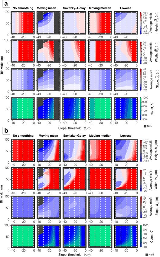
28                                                           M. Hodge et al.: Scarp morphology semi-automated algorithm

numerous events over geological timescales. Linking the           controlling the minimum scale of geomorphic features that
surface offset along the fault to information on the age of the   can be confidently detected.
features can provide information about the rupture and slip          With the current drive toward acquisition of
history on the fault (e.g. Wallace, 1968; Sieh, 1978; Zielke      high-resolution DEMs for paleoseismological stud-
et al., 2012; Ren et al., 2016). For mature faults, it can be     ies (e.g. Zhou et al., 2015; Roux-mallouf et al., 2016;
used to characterise long-term development by identifying         Talebian et al., 2016), two scientific questions arise: (1) what
structural segmentation (e.g. Watterson, 1986; Giba et al.,       DEM resolution is required to successfully locate, calculate
2012; Manighetti et al., 2015) and the presence of linking        and accurately analyse significant changes in displacement
structures (e.g. Soliva and Benedicto, 2004; Nicol et al.,        along a fault scarp; and (2) does our interpretation of the
2010). For faults whose component segments remain uncon-          distribution of displacement scale with DEM resolution (i.e.
nected at the surface, the distribution of displacement along     how much more are we able to infer using an expensive,
a fault can also provide clues to the future structural devel-    high-resolution DEM compared to a free, lower-resolution
opment (e.g. Walsh and Watterson, 1988; Cowie and Scholz,         alternative)?
1992; Dawers et al., 1993; Dawers and Anders, 1995; Pea-             Despite the advances in satellite and computing technol-
cock, 2002) by indicating soft linkages between segments          ogy, and thus the resolution of DEMs, calculating the vertical
(Willemse et al., 1996; Hilley et al., 2001), such as relay       displacement along a scarp is largely a manual process that
ramps. Over time, these segments may hard link; i.e. a con-       has remained consistent over several decades (e.g. Wallace,
nection establishes between segments via rupture of discrete      1977; Bucknam and Anderson, 1979; Avouac, 1993; Wu and
fault planes (e.g. Childs et al., 2017; Hodge et al., 2018b).     Bruhn, 1994; Ganas et al., 2005; Walker et al., 2015). Scarp
Thus, using a combination of the displacement distribu-           height is typically used as a proxy for minimum vertical dis-
tion along a fault and the inter-segment zone geometry,           placement (e.g. Morewood and Roberts, 2001). Scarp height
we can understand what linkage might exist at depth               is typically determined by identifying the fault scarp from an
(e.g. Crider and Pollard, 1998). The importance of distin-        elevation profile, fitting lines to slopes that are on either side
guishing between these two types of linkages is that the          of the scarp and measuring the offset between these fitted
physical connection of a hard link may permit through-going       lines. However, picking the fault scarp location manually can
earthquake rupture and will also increase fluid transport,        be unrepeatable for intermediate- or low-resolution DEMs,
with implications for reservoirs.                                 with measurements showing variability in picked scarp lo-
   In the past, calculating the displacement across a             cation for multiple independent analyses on the same pro-
fault scarp was performed by local field surveys or               files (e.g. Hodge et al., 2018a). Manually processing data
using Global Positioning System (GPS) devices (e.g.               can also be subject to human bias; one person’s definition
Bucknam and Anderson, 1979; Andrews and Hanks,                    of the crest and base of a fault scarp may be different from
1985; Cowie and Scholz, 1992; Gillespie et al., 1992;             another person’s (Middleton et al., 2016). These inconsisten-
Cartwright et al., 1995; Avouac, 1993; Delvaux et al.,            cies ultimately lead to errors within the scarp height calcu-
2012). However, recent advances in remote sensing have            lations and are a contributing factor for the scatter observed
meant that highly accurate and precise vertical displace-         in global maximum displacement-length profiles (Gillespie
ments can be measured using satellite images and digital          et al., 1992) and along-strike displacement profiles (Zielke
elevation models (DEMs) (e.g. Westoby et al., 2012,               et al., 2015).
Bemis et al., 2014, Johri et al., 2014, Zhou et al., 2015,           In this paper, we develop an algorithm that calculates
Roux-mallouf et al., 2016, Talebian et al., 2016). Depending      the parameters (height, width and slope) of a fault scarp
on resolution, DEMs are categorised as low (≥ 30 m),              from a scarp elevation profile: Scarp PARameTer Algorithm
intermediate (∼ 10 m) or high resolution (≤ 5 m). There is        (SPARTA). Using the scarp height as a proxy for vertical
a trade-off between DEM resolution and cost as launching          displacement (e.g. Morewood and Roberts, 2001), a dis-
satellites and acquiring (tasking) images is expensive.           placement profile can be created by calculating scarp height
High-resolution DEMs generated by the newest satellites are       at intervals along a fault scarp. This displacement profile
expensive, exacerbated by large minimum coverage areas            can then be used to infer fault structural segmentation and
(typically ∼ 100 km2 ). Furthermore, generating a DEM             the existence of secondary linking faults (e.g. Crone and
using high-resolution satellite images may require prepro-        Haller, 1991; Cartwright et al., 1995; Dawers and Anders,
cessing steps including pan sharpening and stereo-alignment.      1995; Childs et al., 1996; Giba et al., 2012). Automating the
As a satellite programme becomes discontinued, satellite          morphological calculations will allow a greater number of
images and DEMs are often released for scientific use at          measurements to be taken along a fault scarp than feasible
no cost (e.g. the SPOT Historical archive, Shuttle Radar          with ground based methods, improving the understanding of
Topography Mission). These products require limited to no         fault behaviour and segmentation (e.g. Zielke et al., 2012,
post-processing. Nonetheless, even relatively high-resolution     2015; Trudgill and Cartwright, 1994; Cartwright et al., 1995;
stereo-image derived DEMs have vertical uncertainties, or         Manighetti et al., 2015). Our goal is to develop an algorithm
noise, amounting to around ≥ 30 cm (Zhou et al., 2015),           that is open-source and able to run on a personal computer.

Solid Earth, 10, 27–57, 2019                                                                  www.solid-earth.net/10/27/2019/
M. Hodge et al.: Scarp morphology semi-automated algorithm                                                                     29

We test the performance of the algorithm using a number of         1.1   Normal faults in southern Malawi
synthetic and real fault scarps, for a variety of DEM resolu-
tions.                                                             The Malawi Rift system (MRS) exists at the southern end of
   Algorithms for relative dating of fault scarps, by perform-     the East African Rift system (EARS), extending 900 km from
ing best-fit calculations to a scarp-like template, have already   the Rungwe province in the north to the Urema Graben in the
been attempted (e.g. Gallant and Hutchinson, 1997; Hilley          south (Specht and Rosendahl, 1989; Ebinger et al., 1987).
et al., 2010; Stewart et al., 2017); however, these methods        At the northern end of the rift system is the Mbeya box,
may falsely identify other geomorphic features as fault scarps     which is a triple junction between the Somalia, Victoria and
and require a very high-resolution DEM, usually obtained           Rovuma plates (Ebinger et al., 1989). Rift development com-
using lidar. These autonomous algorithms therefore still re-       menced around approximately 8 Ma (Ebinger et al., 1989)
quire post-processing, manual quality checks. In addition,         with the formation of half-graben units bounded by fairly
Shaw and Lin (1993) developed an algorithm to identify fault       north–south-striking normal faults and propagated from the
scarps by measuring topographic curvature within a moving          north (Ring et al., 1992). Kinematic models of plate motion
window; however, their method only distinguishes between           suggest maximum average extension rates across the Malawi
different relative scarp heights rather than provides a quanti-    Rift of ∼ 3 mm per year, decreasing southwards to less than
tative measurement of scarp height. The algorithm created          2 mm per year (Jackson and Blenkinsop, 1997; Saria et al.,
here (SPARTA) will be developed to be used for a range             2014; Jestin et al., 1994; Stamps et al., 2008). Border fault
of DEM resolutions, where the performance between reso-            systems exist with a predominantly north–south trend at the
lutions is tested in this study.                                   edges of Lake Malawi and alternate sides of the lake at
   Our aim is to develop an algorithm capable of measuring         around 100 km intervals (Rosendahl et al., 1986; Ebinger
along-strike variations in the height of fault scarps at high      et al., 1987).
resolution across a range of settings. The nature of the sub-         In the southern MRS, the Bilila–Mtakataka fault (BMF)
sequent analysis and interpretation will, however, depend on       scarp breaks the surface along almost its entire length, a dis-
the age and type of fault considered as well as the local litho-   tance of ∼ 110 km (Jackson and Blenkinsop, 1997; Hodge
logical and climatic conditions. Individual earthquakes can        et al., 2018a). Early studies suggested that the scarp formed
produce scarps of variable height and a mix of on-fault and        during a single earthquake (Jackson and Blenkinsop, 1997),
off-fault deformation (Wang et al., 2014; Gold et al., 2015;       but the morphology and geometry vary along strike (Hodge
Milliner et al., 2016; Nissen et al., 2016). In some circum-       et al., 2018a) and are more typical of a large, structurally
stances, ruptures are halted by discontinuities or steps in a      segmented normal fault which has experienced several pre-
fault system, whereas other earthquakes produce complex            vious earthquake cycles (e.g. Schwartz and Coppersmith,
rupture patterns which include multiple fault segments (e.g.       1984; Wesnousky, 1986; Peacock and Sanderson, 1991). The
Jackson et al., 1982; Hamling et al., 2017). Between earth-        fault is suggested to comprise six major (first-order) seg-
quakes, erosion depends on variations in lithological and cli-     ments, varying in length from 13 to 38 km, and the distri-
matic properties, which can produce dramatic changes in            bution of scarp height is of two symmetrical bell-shaped pro-
scarp height over short distances in only a few decades. For       files separated by the Citsulo segment (Hodge et al., 2018a).
example, some parts of the scarp formed in the 1981 Alky-          The relatively coarse measurement resolution of the former
onides earthquake, Gulf of Corinth, are well preserved but         studies along the BMF have meant that secondary (second-
others have nearly disappeared (e.g. Mechernich et al., 2018).     order) segments were unable to be identified or characterised,
Some fault scarps are formed by individual earthquakes, oth-       i.e. subordinate segments that have a length of the same or-
ers are multi-scarps produced by a few events, while others        der of magnitude as the major segment they exist within
represent the cumulative effects of numerous earthquake cy-        (Manighetti et al., 2015). Although secondary segments are
cles over tens of thousands of years. In these cases, variations   unlikely to contain gaps of sufficient distance (typically in-
in scarp height may contain information on fault evolution         ferred to be ≥ 6 km) to perturb rupture propagation (e.g.
that can be extracted by identifying structural segmentation       Gupta and Scholz, 2000; Biasi and Wesnousky, 2016), their
(e.g. Watterson, 1986; Giba et al., 2012; Manighetti et al.,       existence may provide evidence for the earliest structural de-
2015) and the presence of linking structures (e.g. Soliva and      velopment of the fault (e.g. Manighetti et al., 2007). Further-
Benedicto, 2004; Nicol et al., 2010). However, these long-         more, understanding structural segmentation is crucial in es-
term effects will be convolved with variations associated with     timating earthquake magnitude, as fault segments may rup-
individual earthquakes. This combination of timescales in-         ture individually, consecutively or continuously (e.g. Ander-
volved in scarp generation raises the question as to what ex-      son et al., 2017; Hodge et al., 2015).
tent variations in offset and erosion persist across multiple         The latest morphological analysis also concludes that there
earthquake cycles.                                                 may be a gap in the BMF scarp across the Citsulo segment
                                                                   (Hodge et al., 2018a). This discontinuity extends for a maxi-
                                                                   mum length of ∼ 10 km. A break in continuity of this length
                                                                   may be sufficient to perturb rupture propagation (Biasi and

www.solid-earth.net/10/27/2019/                                                                   Solid Earth, 10, 27–57, 2019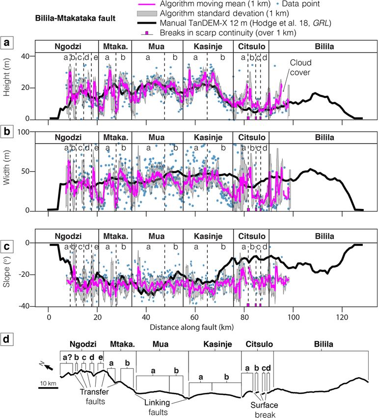
30 M. Hodge et al.: Scarp morphology semi-automated algorithm
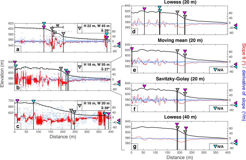
Wesnousky, 2016) and prevent hard linkage along a nor- of the scarp within the data, essentially defined by the scarp
mal fault (Hodge et al., 2018b). A reduced maximum rup- crest and base that bound it. Figure 2a–c show three profiles
ture length would reduce the maximum expected earthquake from the Bilila–Mtakataka fault scarp taken using the 5 m
magnitude (Wells and Coppersmith, 1994) and also the earth- DEM derived from 50 cm Pleiades imagery. The black line
quake repeat time (Hodge et al., 2015). Therefore, in order to shows the elevation data extracted from the DEM, the red
conclude whether the fault scarp is discontinuous across the line shows the change in elevation per unit distance ∂z/∂X
Citsulo segment, and the existence of secondary segments (i.e. slope, θ ), and the blue circles are the derivative of slope
and associated linking faults, a higher-resolution DEM and a ∂ 2 z/∂X 2 (φ). Each of the three profiles is characteristic of
greater number of scarp profiles are required. a different challenge associated with picking the fault scarp
Although the Bilila–Mtakataka fault provides an ideal case manually. The quality of the profile is determined by the
study of a large, continental normal fault, in order to under- non-tectonic features present in the DEM. Profile A has a
stand whether it is unique or representative of early stage rift large, wide scarp that is clearly defined with little ambiguity
faulting, we extend our research to other fault scarps within from other topographic features; however, the gradient of the
the southern, amagmatic MRS. We investigate three addi- scarp is not constant, leading to large slope derivative val-
tional faults in the southern MRS identified during fieldwork, ues (Fig. 2a). Profile B has an ambiguous scarp morphology,
which have previously unreported scarps: the Malombe, Thy- caused by vegetation or other topographical features; these
olo and Muona faults. The Malombe fault is a north–south- features create local variability in slope θ , yet the gradient of
striking, east-dipping normal fault located ∼ 40 km east of the scarp itself is fairly constant (Fig. 2b). Profile C is clear
the Bilila–Mtakataka fault, on the edge of Lake Malombe; of other topographic features, the scarp width is small and
the fault scarp contains at least two major gaps in its surface the magnitude of the change in slope at the fault scarp is not
expression (Fig. 1c). Lithology varies considerably along large; it is therefore difficult to accurately identify the scarp
the fault length, alternating between felsic and mafic parag- from the footwall topography (Fig. 2c). Furthermore, Profile
neisses with fingers of calc-silicate granulite that intersect C’s morphology makes picking a fault scarp even more chal-
the scarp (Manyozo et al., 1972). The Thyolo and Muona lenging when using a lower-resolution DEM.
faults, south of the Bilila–Mtakataka fault, are two overlap- For each profile in Fig. 2, grey triangles denote a manual
ping northwest–southeast-striking, southwest-dipping paral- pick of the crest and base of the fault scarp. These picks are
lel normal fault scarps separated by an offset of ∼ 5 km used to define scarp width. We consider the basic assumption
(Fig. 1d). The lithology of the scarp footwall is very homoge- that the fault scarp represents the approximate position of the
neous at the regional scale, mapped as mafic paragneiss along fault. A linear regression (least-squares method) is then ap-
its entire length (Habgood et al., 1973). Whereas the Bilila– plied to the upper original and lower original surfaces away
Mtakataka, Muona and Thyolo faults all lie in the footwall from the scarp. The best-fitting regression lines for the upper
of a major escarpment at the rift border, the Malombe fault and lower original surfaces (grey dotted lines) are then ex-
is situated near the centre of the rift basin (Fig. 1a). There is trapolated to the point of maximum slope (θmax ) on the iden-
no age control on recent earthquakes on any of these faults, tified fault scarp (Fig. 3). The scarp height H is then taken as
neither are the ages of the escarpments known. To infer the the elevation difference between the regression lines at this
distribution of scarp height, structural segmentation and link- point, the gradient of the best-fit line through the fault scarp
age structures along the Malombe, Thyolo and Muona fault is the scarp slope α, and the horizontal distance between fault
scarps, we develop an algorithm to calculate profiles of the scarp crest and base is the scarp width W .
height and width of the scarp. We then compare our findings Our algorithm picks the crest and base of the fault scarp
for these newly studied faults with the Bilila–Mtakataka fault based on the first and last values of the scarp profile that sat-
and assess their morphology and structural development. We isfy a priori threshold values of slope (θT ) and the derivative
also calculate the slip–length ratio for each fault and compare of slope (φT ). For the algorithm to calculate accurate values
against previously observed values for normal fault earth- for scarp height, width and slope, the thresholds need to be
quakes (Scholz, 2002). appropriate for the scarp’s morphology; i.e. for gently dip-
ping fault scarps, the slope threshold should also be of a gen-
tle angle. Two examples for slope threshold are shown for the
2 The SPARTA algorithm profiles in Fig. 2: one where the slope threshold is set to 20◦
(pink triangles) and one where it is 40◦ (blue triangles). For
2.1 Algorithm development all profiles, neither threshold value performs well at automat-
ically identifying a fault scarp equivalent to the one that was
2.1.1 Scarp identification determined manually. The reason for the poor algorithm per-
formance is ambiguity in the scarp morphology, where non-
For a given profile perpendicular to the local scarp trend, the tectonic features may lead to the misidentification of the fault
first step in calculating the scarp’s morphological parame- scarp by the algorithm. For example, in Fig. 2a and c, the al-
ters (height, width and slope) is to identify the exact position gorithm fails to accurately identify the base of the fault scarp
Solid Earth, 10, 27–57, 2019 www.solid-earth.net/10/27/2019/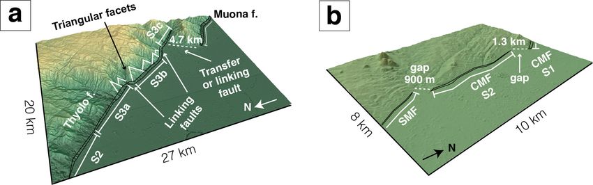
M. Hodge et al.: Scarp morphology semi-automated algorithm 31
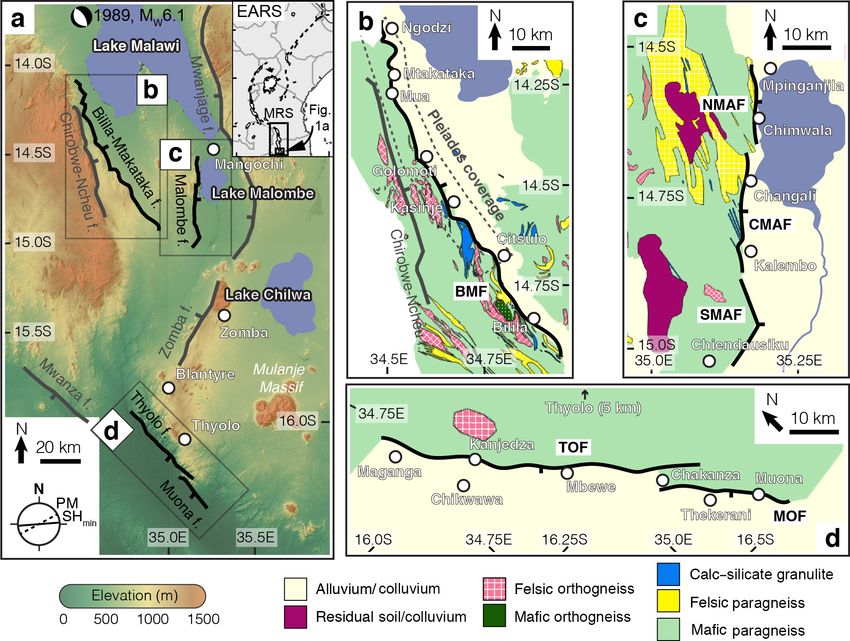
Figure 1. (a) Map of faults in southern Malawi; those used in this study are coloured black. Tick marks show the dip direction. Lower left
corner shows the plate motion (PM; 86◦ ± 5◦ ) from Saria et al. (2014) and local minimum horizontal stress (SHmin ; 62◦ ) from Delvaux
and Barth (2010). Top right corner shows the location with respect to the East African Rift system (EARS) and Malawi Rift system (MRS).
Panels (b)–(d) are geological maps of (b) the Bilila–Mtakataka fault (BMF) showing the coverage of the Pleiades satellite imagery (taken
from Walshaw, 1965; Dawson and Kirkpatrick, 1968); (c) the Malombe fault (MAF): northern Malombe fault (NMAF), central Malombe
fault (CMAF) and southern Malombe fault (SMAF) (taken from Manyozo et al., 1972); and (d) the Thyolo fault (TOF) and Muona fault
(MOF) (taken from Habgood et al., 1973).
due to irregularities in the lower original surface. For all ex- For the moving mean and moving median filters, we use
amples, the crest of the fault scarp is misidentified by the the rolling mean algorithm from the pandas Python module
algorithm due to topographic features within the upper orig- and the moving median algorithm from the SciPy Python
inal surface. Furthermore, as the values of φ have a higher module, respectively. Both filters are commonly used signal-
amplitude than θ , the algorithm is more sensitive to the slope processing algorithms because they are the easiest and fastest
derivative threshold than the slope threshold. To enhance the digital filters to understand and use. In image processing, the
clarity of the elevation profiles, we apply and test a range of median filter is usually the preferred digital filter to repre-
digital filters that will essentially remove non-tectonic fea- sent an average. This is because an individual unrepresen-
tures from the data. tative value in the window will not affect the median value
as significantly as it affects the mean. However, the median
2.1.2 Filtering filter also preserves sharp edges and therefore may lead to
step-like features, which could cause steep slope artefacts in
Here, we test the suitability of four digital filters (mov- our profiles. The Savitzky–Golay filter is based on a local
ing mean, moving median, Savitzky–Golay and Lowess) in least-squares polynomial approximation (Savitzky and Go-
smoothing out non-tectonic features in the scarp profiles and lay, 1964); it is less aggressive than simple moving filters and
improving the accuracy with which morphological parame- is therefore better at preserving data features such as peak
ters such as height and width can be extracted by automated height and width. The Lowess filter uses a non-parametric
processing. Each filter uses a moving window over a spec- regression method and requires larger sample sizes than the
ified bin width, which must be an odd integer. The moving other filters (Cleveland, 1981). The Lowess filter can be per-
window is incrementally shifted along the profile for each formed iteratively, but since it requires much more computa-
data point.
www.solid-earth.net/10/27/2019/ Solid Earth, 10, 27–57, 2019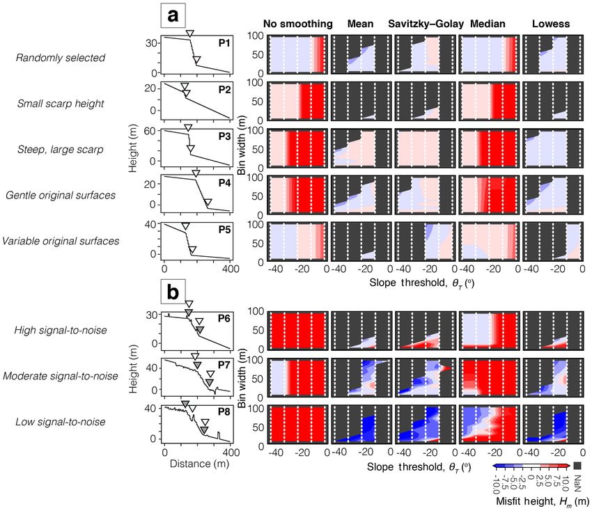
32                                                                  M. Hodge et al.: Scarp morphology semi-automated algorithm

Figure 2. Panels (a) to (c) show three profiles across the Bilila–Mtakataka fault scarp using the Pleiades 5 m DEM. Each is characteristic
of the different challenges associated with picking the fault scarp manually and using an algorithm. Profile A has a clearly defined scarp,
although the scarp itself contains non-tectonic topographic features making it difficult to quantify its shape. Profiles B and C have more
distributed topographic noise, and Profile C has a scarp that is difficult to accurately identify as the magnitude of the change in slope at the
fault scarp is not large. Using Profile B, four different digital filters and/or bin widths were applied: (d) Lowess (bin width 20 m); (e) moving
mean (bin width 20 m); (f) Savitzky–Golay (bin width 20 m); and (g) Lowess (bin width 40 m). The black line is the elevation profile, the red
line is the slope (θ ) profile, and blue circles denote the derivative of slope (φ). Grey triangles show the location of the crest and base of the
fault scarp based on a manual pick. Pink and blue triangles denote the algorithm’s pick of the crest and base based on a slope threshold of
20◦ (pink) and 40◦ (blue), respectively.

tional power than the other filter methods, we apply a single              width. By smoothing the data, the relative amplitude of φ
pass over the data.                                                        becomes smaller than that of θ , meaning that the algorithm
   Figure 2d–g show the results of applying a digital filter               becomes less sensitive to the slope derivative threshold than
to Profile B (Fig. 2b). This profile was chosen because of                 the slope threshold. For the same bin width (20 m), the algo-
the extensive topographic variation within the upper origi-                rithm using the Lowess and Savitzky–Golay filters estimates
nal surface. Such irregularity is typical for fault scarp pro-             the scarp location more accurately than the moving mean for
files, as topographic features from previous deformation                   this profile, as the latter fails to significantly reduce the ambi-
events, valleys and dense vegetation are common. The el-                   guity caused by non-tectonic features within the upper origi-
evation data were filtered using the following parameters:                 nal surface; however, for all filters, the algorithm still falsely
(d) Lowess (bin width 20 m); (e) moving mean (bin width                    identifies the crest of the fault scarp using a slope threshold
20 m); (f) Savitzky–Golay (bin width 20 m); and (g) Lowess                 of 20 or 40◦ . The algorithm using a slope threshold of 20◦
(bin width 40 m). Filter parameters for Profiles D, E and F                performs reasonably well once the profile has been filtered
were chosen as a comparison between three different filter                 using the Lowess filter and a bin width of 40 m (Fig. 2f), for
methods using the same bin width, whilst parameters for Pro-               this example.
files D and G were chosen for a comparison between differ-                     The Lowess filter smooths the elevation, and subsequently
ent bin widths for the same filter method.                                 the profiles of slope θ and slope derivative φ, more than the
   The Lowess and Savitzky–Golay filters smooth the ele-                   moving mean filter. As expected, a larger bin width smooths
vation, and subsequently the profiles of slope θ and slope                 the data more than a smaller bin width. By smoothing the
derivative φ, more than the moving mean filter. As expected,               data, the relative amplitude of φ becomes smaller than that of
a larger bin width smooths the data more than a smaller bin                θ , meaning that the algorithm becomes less sensitive to the

Solid Earth, 10, 27–57, 2019                                                                              www.solid-earth.net/10/27/2019/
M. Hodge et al.: Scarp morphology semi-automated algorithm                                                                             33

slope derivative threshold than the slope threshold. For the
same bin width (20 m), the algorithm using the Lowess filter
estimates the scarp location more accurately than the mov-
ing mean for this profile, as the latter fails to significantly
reduce the ambiguity caused by non-tectonic features within
the upper original surface; however, for both filters, the algo-
rithm still falsely identifies the crest of the fault scarp using
a slope threshold of 20 or 40◦ . The algorithm, using a slope
threshold of 20◦ , performs reasonably well once the profile
has been filtered using the Lowess filter and a bin width of
40 m (Fig. 2f), for this example.

2.2   Assessing algorithm performance

We assess the performance of our algorithm by testing it on         Figure 3. An example of a synthetic catalogue fault scarp. (a) Vi-
various scarp profiles. Performance is assessed by defining         sual description of the parameters in Table 1 used in the syn-
a misfit value for scarp height (Hm ), width (Wm ) and slope        thetic catalogue without non-tectonic features. (b) The difference
(αm ) as the difference between ground-truthed (Hg , Wg , αg )      between vertical displacement Z and synthetic profile scarp height
and algorithm-calculated (Hc , Wc , αc ) scarp parameters –         Hg , resulting from sloping original surfaces. (c) The additional non-
                                                                    tectonic synthetic catalogue parameters (H indicates hills; V indi-
based on the selected a priori parameters b, θT , φT and fil-
                                                                    cates vegetation; D indicates ditches) and diffusion (red indicates
ter method – for each profile. Misfit values can be positive
                                                                    erosion; green indicates deposition).
or negative. This approach relies on the assumption that the
ground-truthed value is correct and is the value that we want
the algorithm to calculate. One approach, as shown above, is                    n
                                                                             1X
to use a manual analysis to calculate the ground-truthed val-       Wm =           Wc(i) − Wg(i)                                      (2)
                                                                             n i=1
ues. For example, for Profile G the crest and base were both
                                                                               n
identified by the algorithm within 5 m of the manual pick,                  1X
                                                                    αm =          αc(i) − αg(i)                                       (3)
leading to a height misfit of less than 1 m, a width misfit of              n i=1
less than 6 m and a slope misfit smaller than 1◦ (Fig. 2g).
Another way to test algorithm performance is to generate a                |H m | + |W m | + |α m |
                                                                    ε=                             , for C ≥ 0.5 n                    (4)
synthetic fault scarp profile where the ground-truthed values                      C/n
are the input parameters.
   Although the ultimate goal is to design an algorithm to cal-
                                                                    3     Synthetic tests
culate scarp parameters for real fault scarps, the creation of
a synthetic catalogue will allow us to robustly test the algo-      3.1    Synthetic catalogue
rithm, and the relationship between filter and threshold pa-
rameters, using a large number of scarp profiles. This would        In order to test the possible combinations of filtering, bin
not be feasible using the manual process. Therefore, the algo-      sizes, etc. using a Monte Carlo approach, we construct two
rithm is run iteratively on a number (n) of synthetic profiles,     synthetic catalogues, with and without non-tectonic features
using a range of a priori filter and threshold values. Average      causing topographic noise in the DEM, each comprising
height (H m ), width (W m ) and slope (α m ) misfit values are      1000 fault scarp profiles.
then calculated using the mean of individual misfit values             The parameters used in the construction of both catalogues
from the profiles (Eqs. 1 to 3). The total number of profiles       are the location of the scarp crest along the profile (xs ), the
where a fault scarp is identified by the algorithm is given         slope of the upper original surface (βu ) and the slope of the
as the count C. The total misfit value, ε, is then calculated       lower original surface (βl , Table 1; Fig. 3a). Profile length
using Eq. (4); all algorithm runs where the number of fault         x and resolution r are constants set to 400 and 1 m, respec-
scarps identified is fewer than 50 % are removed. Although          tively. Parameters βu and βl could be omitted if the synthetic
calculating the correct scarp height is the most important ele-     catalogue is used to mimic an environment where fault scarps
ment of our algorithm, an equal weight is applied to all scarp      offset flat surfaces (e.g. Borah Peak fault scarp, Idaho; Ward
parameters because all contribute to how well the scarp is          and Barrientos, 1986) and included for regions where fault
identified. The smallest ε value is then used to denote the         scarps offset sloped surfaces (e.g. Mangola fault scarp, cen-
best-performing set of filter and threshold parameters.             tral Apennines; Tucker et al., 2011). A down-dip, normal
          n
                                                                    sense of displacement parallel to the scarp is then imposed,
       1X                                                           and Z and X are defined as the vertical (throw) and horizontal
Hm =         Hc(i) − Hg(i)                                   (1)
       n i=1                                                        (heave) components of this displacement. The synthetic fault

www.solid-earth.net/10/27/2019/                                                                        Solid Earth, 10, 27–57, 2019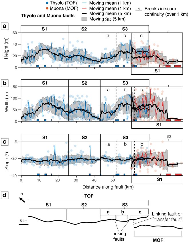
34                                                            M. Hodge et al.: Scarp morphology semi-automated algorithm

scarp width Wg therefore equals the horizontal displacement            Figure 4a shows five examples with various morpholo-
X and scarp slope αg equals tan−1 (Z/X). The height of the         gies from the synthetic catalogue without non-tectonic to-
synthetic fault scarp Hg is then calculated using Eq. (5). The     pographic features: (P1) randomly selected; (P2) small scarp
larger the values of βu and βl , the larger the difference be-     height; (P3) steep, large scarp; (P4) gently dipping, parallel
tween measured throw and actual throw, Hg and Z (Fig. 3b).         original surfaces; and (P5) non-parallel original surfaces. The
                                                                   algorithm was tested using all combinations of filter meth-
           X
Hg = Z −     (tan βu + tan βl )                             (5)    ods, bin widths and slope thresholds. For each profile, misfit
           2                                                       values were calculated (Fig. 4a). For scarp width and slope
   The noisy catalogue includes irregularities in the form of      misfit for synthetic catalogues, see the Supplement. For all
non-tectonic topographic features such as vegetation, hills        examples, the algorithm was able to identify a fault scarp
and ditches, as well as scarp degradation by diffusion (Ta-        and report scarp height with a misfit of less than 2.5 m (5 %–
ble 1; Fig. 3c). A random number of these non-tectonic fea-        60 % of the scarp height for some combination of param-
tures are placed at random locations along the profile. The        eters); however, for Profile 2, the algorithm was unable to
shape of these features is a negative parabola between a and       identify a fault scarp when the bin width was greater than
b, created using Eq. (6), where a is the first root at the ran-    30 m. In this case, the filter was too aggressive and over-
dom location and b is the second root at a horizontal distance     smoothed the scarp, such that no clear break in slope was
from the first root equating to the feature width, with a height   detectable. Detectability of the scarp slope is a function of
−kb2                                                               resolution, scarps may not be identified if the bin width is
  4 .
                                                                   3 times the scarp width and height, and the misfit values are
y = −k(x − a)(x − a − b)                                    (6)    greater for bin widths twice the scarp width and/or height.
                                                                       To illustrate the process, we chose three examples from the
   Diffusion is applied in a Monte Carlo approach by using
                                                                   noisy synthetic catalogue based on their topographic irregu-
Eq. (7) for a diffusion constant κ and time t, resulting in ero-
                                                                   larity and diffusion parameters (Fig. 4b). Profile 6 includes
sion of material from the upper portion of the scarp and de-
                                                                   lots of vegetation but no hills or ditches, nor any scarp diffu-
position at the base (Fig. 3c). Diffusion can be included for
                                                                   sion. Profile 7 includes hills, ditches and scarp diffusion but
environments where hillslopes are mantled with a continu-
                                                                   no vegetation. Profile 8 includes vegetation, hills and ditches
ous soil cover (i.e. transport-limited) and excluded for those
                                                                   and therefore has the largest amount of topographic noise
with extensive areas of bare bedrock (i.e. weathering-limited)
                                                                   and also includes scarp diffusion. For all three profiles, us-
(e.g. Tucker et al., 2011; Bubeck et al., 2015; Boncio et al.,
                                                                   ing no filter or the moving median filter gave the largest mis-
2016). Early studies of scarp degradation suggested that the
                                                                   fit values (Fig. 4b). For scarp width and slope misfit, see the
value of κ should typically be between 0.5 and 1.5 m2 kyr−1
                                                                   Supplement. The moving mean filter provided a small scarp
(e.g. Hanks et al., 1984; Andrews and Hanks, 1985; Arrow-
                                                                   height misfit (< 2.5 m) for Profiles 6 and 7, but produced a
smith et al., 1996); however, recent studies from Mongolia
                                                                   larger misfit (Hm > 7.5 m) for Profile 8. The Savitzky–Golay
(Carretier et al., 2002), the Gulf of Corinth (Kokkalas and
                                                                   and Lowess filters performed equally well on all profiles,
Koukouvelas, 2005) and the upper Rhine Valley (Nivière and
                                                                   with the former able to identify fault scarps with a slightly
Marquis, 2000) have suggested κ values in the range of 3 to
                                                                   larger bin width and steeper slope threshold than the latter.
10 m2 kyr−1 . Locally on scarps in the Gulf of Corinth, κ has
been measured to be as low as 0.2 m2 kyr−1 (Kokkalas and
                                                                   3.3   Exploration of parameter space using synthetic
Koukouvelas, 2005); however, errors in calculations can be
                                                                         catalogue
as large as 0.5 m2 kyr−1 . Here, we set algorithm limits to 0.5
and 10 m2 kyr−1 .
                                                                   For each of the 1000 profiles in the synthetic catalogues, we
dh        d2 h                                                     test 250 unique combinations of algorithm parameters (filter
   =κ· 2                                                    (7)    method, bin width and slope threshold) and assess their abil-
dt    dx
                                                                   ity to accurately determine the synthetic input parameters.
                                                                   Where the algorithm is not able to identify a fault scarp, a
3.2   Individual profiles                                          result is not recorded.
                                                                      Figure 5a shows the average misfit values for the noise-
We test the performance of the algorithm by comparing              free synthetic profiles where the algorithm identified a fault
ground-truthed synthetic scarp values to scarp parameter val-      scarp (Eqs. 1 to 3). The best-performing bin width and slope
ues calculated by the algorithm. The synthetic catalogue in-       threshold depended on the filter method used, but in gen-
put values are shown in Table 1. All filters from Sect. 2.1.2      eral a smaller bin width and steeper slope threshold provided
were tested, using a bin width between 9 and 99 m, increasing      smaller misfit values. When not applying a filter, or using
in increments of 10 m. We vary slope threshold, θT , between       the median filter, the algorithm performed poorly; but using
1 and 41◦ , in increments of 10◦ , and fix the slope derivative    these filters meant the fault scarp was identified in more pro-
threshold, φT , to 5◦ m−1 .                                        files. For the moving mean, Savitzky–Golay and Lowess fil-

Solid Earth, 10, 27–57, 2019                                                                  www.solid-earth.net/10/27/2019/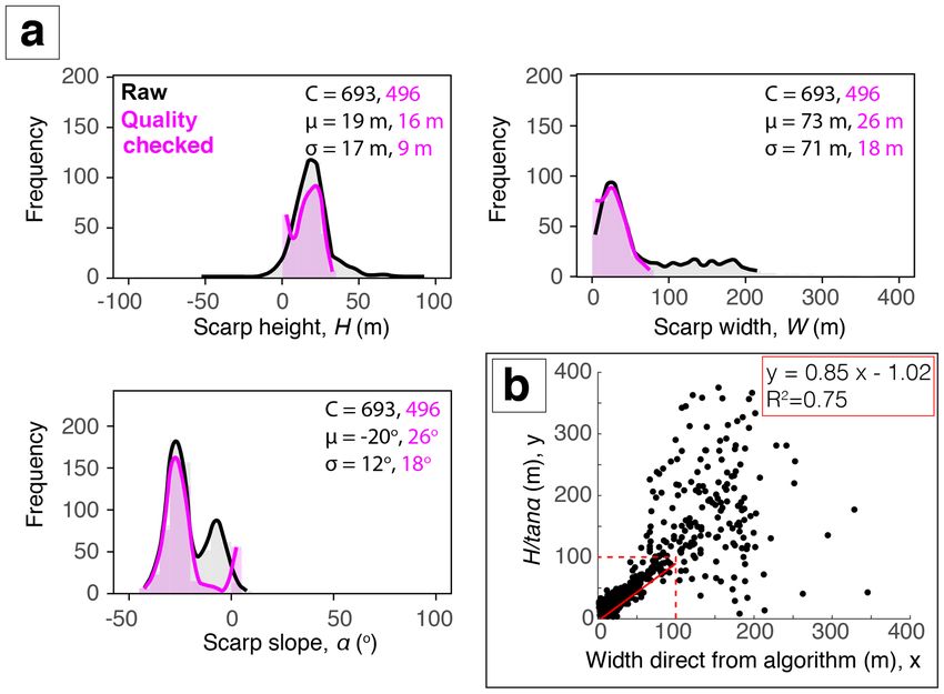
M. Hodge et al.: Scarp morphology semi-automated algorithm                                                                             35

Table 1. Parameters used in creating the synthetic catalogues.

                                       Algorithm parameters                                This study
                          Parameter              Symbol     Unit               Minimum value     Maximum value
                          All catalogue parameters
                          Profile length         x          metres (m)                     400                 –
                          Scarp location         xs         metres (m)                     100               300
                          Vertical offset        Z          metres (m)                       2                50
                          Horizontal offset      X          metres (m)                       2               100
                          Upper slope            βu         degrees (◦ )                     5                 0
                          Lower slope            βl         degrees (◦ )                     5                 0
                          Additional non-tectonic topographic parameters
                          Diffusion constant     κ          m2 kyr−1                       0.5                10
                          Chronological age      t          kyr                              0                50
                          Vegetation number      vn         dimensionless                    0                20
                          Vegetation height      vH         metres (m)                       1                 3
                          Vegetation width       vW         metres (m)                       1                 3
                          Hill number            hn         dimensionless                    0                 3
                          Hill height            hH         metres (m)                       3                10
                          Hill width             hW         metres (m)                       8                15
                          Ditch number           dn         dimensionless                    0                 3
                          Ditch depth            dH         metres (m)                       3                10
                          Ditch width            dW         metres (m)                       8                15

ters, a gentle slope threshold (θT < 11◦ ) gave large misfit val-          DEM for an area of the Bilila–Mtakataka fault scarp. The
ues, but using a steep threshold (θT ≥ 31◦ ) meant fault scarps            scarp trace was manually picked from each hillshade image
were identified in less than 50 % of the profiles.                         and is shown by a red line. Large-scale changes in scarp trend
   The poor algorithm performance when not using a filter,                 can be identified using the SRTM DEM (box A; Fig. 6); how-
or using the moving median filter, is apparent for the average             ever, small-scale changes may not be identifiable (boxes B
misfit values using the noisy catalogue (Fig. 5b). On aver-                and C; Fig. 6).
age, the scarp width misfit values are larger than the scarp                  We use the station lines toolbox in QGIS to draw profile
height misfit values. Whereas scarp height is estimated by                 lines perpendicular to the manually picked fault scarp trace.
linear extrapolation of the original surfaces and is therefore             The total length of profile x was set to 400 m. To obtain
less influenced by non-tectonic topographic features and ex-               accurate calculations of the scarp’s morphological parame-
act position of the fault scarp, scarp width is highly sensitive           ters (especially width and slope), profiles need to be taken
to the exact location of the fault scarp crest and base picked             perpendicular to the scarp trend. Therefore, where the scarp
by the algorithm.                                                          trend varies considerably, such as at the ends of fault seg-
   For both synthetic catalogs, the best-performing filters                ments and at linking structures, failing to account for the
were the Savitzky–Golay and Lowess filters; the slope                      small changes in scarp trend may lead to inaccurate morpho-
threshold with the smallest total misfit (Eq. 4) was 21◦ , and a           logical measurements. To prevent the station lines from being
bin width of 50 m or smaller was found to perform better than              drawn oblique to the true fault scarp, resulting from small-
a larger bin width. Thus, these are the optimal filters which              scale changes in scarp geometry, the distance between nodes
we choose to employ on the real data, using bin width and                  (points picked on the fault scarp that when joined represent
slope thresholds tailored to the local environment.                        the scarp trace) should be significantly less than the distance
                                                                           between profiles. Here, we select scarp-perpendicular pro-
                                                                           files at intervals of 100 m along the fault scarp trace and
4   Case study example: the Bilila–Mtakataka fault                         therefore use a nodal distance of ∼ 20 m. Therefore, as the
                                                                           resolution of the TanDEM-X DEM is smaller than the nodal
For the Shuttle Radar Topography Mission (SRTM),                           distance, we use this to pick the surface trace of the Bilila–
TanDEM-X and Pleiades DEMs, hillshade and slope maps                       Mtakataka fault scarp.
were produced in QGIS 2.18 and used to identify the breaks                    A total of 913 scarp profiles were extracted from the
in slope associated with the Bilila–Mtakataka fault, i.e. the              SRTM, TanDEM-X and Pleiades 5 m DEMs, for ∼ 90 km
scarp. Figure 6 shows the hillshade image produced by each

www.solid-earth.net/10/27/2019/                                                                           Solid Earth, 10, 27–57, 2019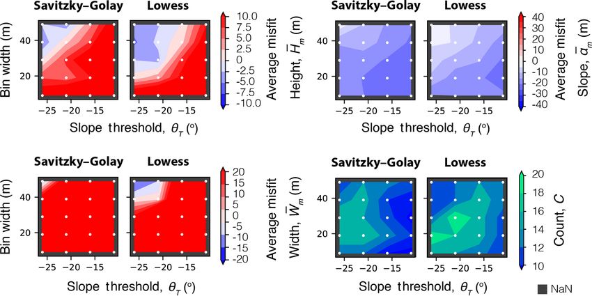
36                                                                 M. Hodge et al.: Scarp morphology semi-automated algorithm

Figure 4. Scarp height misfit Hm for (a) five synthetic catalogue examples with no non-tectonic features and (b) three synthetic catalogue
examples with noise in the DEM caused by non-tectonic features. See the Supplement for scarp width Wm and slope misfit αm results for the
catalogues with and without non-tectonic topographic features. As with Fig. 2, grey triangles show the location of the crest and base of the
fault scarp based on the input parameters. White triangles denote the algorithm’s best pick of the crest and base based on the misfit analysis.

of the Bilila–Mtakataka fault scarp that was covered by the                  Based on the algorithm performance in the synthetic tests,
Pleiades DEM, starting ∼ 7.4 km from the northern fault                   we only use the Savitzky–Golay and Lowess filters. The
end (Fig. 1b). Due to clouds over the fault scarp on the                  maximum bin width is reduced to 49 m, and slope thresh-
Pleiades optical images, 26 profiles between 94 and 97 km                 old limits are 11 and 26◦ , with increments of 5◦ . We find that
from the northern fault end were removed. Elevation values                the algorithm using the Lowess filter, on average, had smaller
were taken along each profile at a spacing equal to the reso-             misfit values and identified a greater number of fault scarps
lution of the DEM (e.g. 5 m for the Pleiades DEM).                        than that using the Savitzky–Golay filter (Fig. 8). As with the
                                                                          synthetic tests, larger bin widths and steeper slope thresholds
                                                                          generated smaller misfit values, especially for scarp width;
4.1   Algorithm results (Pleiades 5 m DEM)
                                                                          however, they also identified fewer fault scarps. The algo-
                                                                          rithm using the Savitzky–Golay filter gave a large width mis-
To test the algorithm using a range of resolution datasets                fit (> 20 m), except when using the largest bin widths and
we first use the Pleiades profiles along the Bilila–Mtakataka             steepest slope thresholds in the study. Based on the total mis-
fault. A manual analysis is conducted for 20 profiles, taken at           fit value, the best results were achieved by the Lowess fil-
increments of ∼ 5 km along the Bilila–Mtakataka fault scarp               ter when bin width is 39 m, and a slope and slope derivative
(Fig. 7). A misfit analysis is performed by comparing scarp               thresholds were 21 and 5◦ m−1 , respectively. The average
parameters estimated manually and from the automated anal-                misfit values using this algorithm setup were H m = 1.4 m,
ysis.

Solid Earth, 10, 27–57, 2019                                                                            www.solid-earth.net/10/27/2019/
M. Hodge et al.: Scarp morphology semi-automated algorithm 37 Figure 5. The average misfit and count for 1000 (a) noise-free and (b) noisy synthetic catalogue fault scarps, where by “noise” we refer to non-tectonic topographic features leading to ambiguity in the DEM. Grey values denote no fault scarp was identified for all profiles. For resolutions of 5, 10 and 30 m, see the Supplement. W m = −6.6 m and α m = −12.6◦ . These values are specific Using the best-performing parameters, the algorithm was to this example and would vary according to DEM resolu- able to identify a fault scarp for 79 % of the 913 profiles. A tion, scarp characteristics and location. histogram of the scarp height, width and slope, as well as the www.solid-earth.net/10/27/2019/ Solid Earth, 10, 27–57, 2019
38                                                               M. Hodge et al.: Scarp morphology semi-automated algorithm

Figure 6. Bilila–Mtakataka fault scarp hillshade DEM examples using SRTM 30 m, TanDEM-X 12 m and Pleiades 5 m DEMs. The black
arrows represent the fault scarp trace picked using each DEM. Box A represents the typical trend of the Bilila–Mtakataka fault scarp, boxes
B and C show changes in variation in scarp trend.

                                                                        4.1.1   Resolution analysis

                                                                        Manual analyses were performed for the 20 chosen profiles
                                                                        along the Bilila–Mtakataka fault scarp using the TanDEM-
                                                                        X and SRTM DEMs, and compared to the Pleiades DEM
                                                                        manual results (Fig. 7). Scarp height estimates between man-
                                                                        ual analyses differed by a maximum of 18 m, width by up to
                                                                        60 m and slope by up to 24◦ , but the average differences were
                                                                        much lower: ∼ 4 m, ∼ 13 m and ∼ 8◦ , respectively. The cal-
                                                                        culated scarp height and slope were the smallest and most
                                                                        gentle using the SRTM DEM, and tallest and steepest using
                                                                        the Pleiades DEM, likely due to the differing DEM resolu-
                                                                        tions.
                                                                           The algorithm was then run for the 913 fault scarps using
                                                                        the TanDEM-X and SRTM DEMs, using the best-performing
Figure 7. Manual Bilila–Mtakataka fault profile for (a) height H ,      algorithm setup found for the Pleiades analysis. For plots
(b) width W and (c) slope α taken at ∼ 5 km intervals using the         from this resolution analysis, see the Supplement. Although
Pleiades 5 m, TanDEM-X 12 m and SRTM 30 m DEMs. For tabular             the misfit values were comparable regardless of DEM reso-
results, see the Supplement.                                            lution, the lower the resolution, the fewer fault scarps were
                                                                        identified: 69 % for TanDEM-X and 64 % for SRTM, com-
                                                                        pared with 79 % for Pleiades. The standard deviation of re-
mean and standard deviation (σ ), is shown in Fig. 9a (black).
                                                                        sults was smaller for both TanDEM-X and SRTM results than
The average Bilila–Mtakataka fault scarp height, width and
                                                                        the Pleiades DEM, leading to fewer outliers being removed
slope were 19 m (±17 m), 73 m (±71 m) and 20◦ (±12◦ ),
                                                                        after the quality-check tests were performed. Misfit values
respectively. However, as the standard deviation was of the
                                                                        were smaller using the higher-resolution DEMs. In agree-
same order of magnitude as the values themselves, this sug-
                                                                        ment with the manual analysis, the algorithm scarp param-
gests there was a wide spread of results due to natural vari-
                                                                        eters were smaller, wider and more gentle on average using
ability. Furthermore, the extremes exceeded the minimum
                                                                        the SRTM DEM, but the algorithm was still able to identify
and maximum values obtained in the manual analysis.
                                                                        scarps with heights less than 5 m.
                                                                           The average scarp height, width and slope obtained
                                                                        through the algorithm using each DEM were similar. The
                                                                        difference in scarp height between resolutions was smallest
                                                                        between Pleiades and TanDEM-X (2σ < 10 m) and largest
                                                                        between TanDEM-X and SRTM (2σ ∼ 12 m). The greatest
                                                                        difference in algorithm performance between resolutions was
                                                                        found for scarp width (40 m > 2σ > 20 m), whereas the dif-

Solid Earth, 10, 27–57, 2019                                                                         www.solid-earth.net/10/27/2019/
M. Hodge et al.: Scarp morphology semi-automated algorithm 39
Figure 8. Average misfit values between algorithm and manual scarp parameters for 20 Bilila–Mtakataka fault profiles using the Pleiades
5 m DEM.
and for accurate slope calculations, a high-resolution DEM
is more appropriate.
5 Application to Malombe, Thyolo and Muona faults
We have shown that an automated approach performs well
in comparison to a manual analysis for the Bilila–Mtakataka
fault scarp. We now apply the algorithm to three further
normal fault scarps: the Malombe, Thyolo and Muona fault
scarps in southern Malawi (Fig. 1). The Thyolo fault (TOF)
and Muona fault (MOF) are two distinct, overlapping fault
scarps. As such, they may be part of the same fault system;
however, a physical connection between them is not obvious
in the TanDEM-X DEM. The Malombe fault (MAF) is split
into three scarps: the northern (NMAF), central (CMAF)
Figure 9. (a) Histogram of the estimated scarp parameters for the and southern (SMAF) scarps. As the algorithm performed
Bilila–Mtakataka fault for all (raw) algorithm estimates (black) and comparatively well using TanDEM-X DEM and the Pleiades
post-quality-checked (pink) results. (b) A comparison between the DEM for the Bilila–Mtakataka fault, we can reliably use
scarp width obtained directly from the algorithm and the scarp
TanDEM-X where Pleiades is not available. Therefore, for
width calculated using the algorithm’s scarp height and slope val-
ues (Wc = Hc / tan αc ). A linear regression is applied where width
each fault, scarp parameters were calculated using the al-
is less than 100 m. gorithm from 400 m long scarp-perpendicular profiles taken
using the TanDEM-X DEM. Nodal distance for the manu-
ally picked scarp traces is again set to ∼ 20 m and scarp-
perpendicular profiles are taken at intervals of 100 m. For
ference between scarp slope using each resolution typically each, we select a subsample of 25 scarp profiles for a mis-
was less than 15◦ . The difference in scarp height between res- fit analysis against a manual method (Eqs. 1 to 4) and limit
olutions did not show any clear along-strike pattern and was our filter methods to Savitzky–Golay and Lowess.
on average less than 5 m. Using a moving mean, the along-
strike changes in scarp parameters between DEMs are sim- 5.1 Scarp morphology of Malombe, Thyolo and Muona
ilar and match the manual analyses well. For a scarp whose faults (TanDEM-X 12 m DEM)
height is comparable to that of the Bilila–Mtakataka’s, we
find that using a low-resolution DEM (i.e. 30 m SRTM) does The Thyolo fault scarp is ∼ 70 km long and trends predomi-
not profoundly affect the results; however, for smaller scarps nantly northwest–southeast (Fig. 1c). Results from the man-
www.solid-earth.net/10/27/2019/ Solid Earth, 10, 27–57, 201940 M. Hodge et al.: Scarp morphology semi-automated algorithm
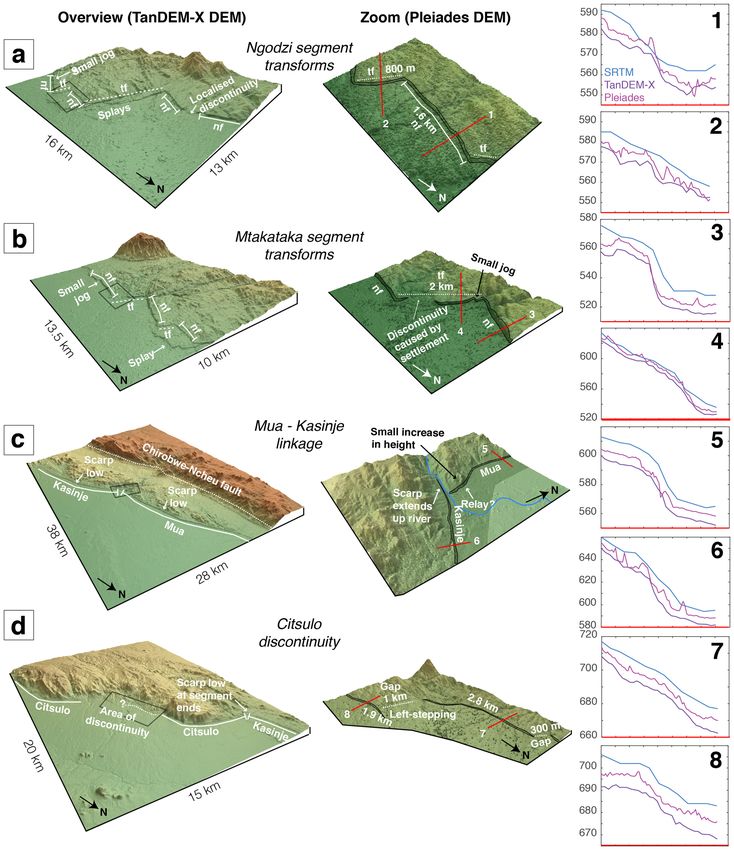
Figure 10. Panels (a)–(c) show the height, width and slope profiles for the Bilila–Mtakataka fault scarp using the Pleiades DEM, indicating
the major segments proposed in Hodge et al. (2018b) (Ngodzi, Mtakataka, etc.) and newly identified secondary segments (a, b, etc.) from
this study. (d) A map view showing fault structural segmentation, breaks in scarp and the location of inferred linkage structures.
Table 2. The best-performing algorithm parameters for the Thyolo, Muona and Malombe faults based on a misfit analysis using the TanDEM-
X DEM: Lowess (LW) or Savitzky–Golay (SG).
Fault name Filter θ b H m (m) W m (m) α m (◦ ) Count, C (%)
TOF LW 19 41 6.2 −1.5 −0.6 60 %
MOF SG 23 29 11.9 −2.3 −6.0 52 %
NMAF SG 15 21 1.1 −4.1 −0.8 52 %
CMAF SG 15 29 8.4 2.3 −6.7 52 %
SMAF LW 7 9 5.8 −13.3 1.8 56 %
ual analysis indicate that the average height of the TOF scarp and more gentle (14◦ on average) than the TOF fault. The
is ∼ 18 m, and its average slope is 18◦ . For results, see the scarp width for both faults was ∼ 65 m on average, equiva-
Supplement. The scarp of the parallel Muona fault steps lent to ∼ 5 pixels. The scarp height for both faults increases
to the right of the Thyolo fault and is shorter, measuring by up to ∼ 9 m km−1 toward the overlap zone. Scarp mea-
∼ 28 km long. The faults overlap for a distance of ∼ 10 km surements for the TOF within the overlap zone may contain
and are separated by ∼ 5 km (Fig. 1c). The manual analy- significant errors due to the complex topography within the
sis suggests that the MOF scarp is lower (10 m on average) footwall of the Muona scarp affecting the linear regression
Solid Earth, 10, 27–57, 2019 www.solid-earth.net/10/27/2019/M. Hodge et al.: Scarp morphology semi-automated algorithm 41
of original surfaces. The best-performing filter for the TOF strike profile. The ability to measure scarp parameters at a
was the Lowess filter, whereas the Savitzky–Golay filter per- high spatial resolution is a major benefit of an automated
formed better for the Muona scarp (Table 2). Both faults re- algorithm. Using the traditional, manual approach, increas-
quired similar slope thresholds, but the TOF required a larger ing the number of fault scarp profiles would dramatically in-
bin width (41 m compared to 29 m). The algorithm misfit val- crease the time required.
ues for the subsampled profiles are shown in Table 2. The In addition, by increasing the spatial resolution of mea-
algorithm performed less well for the MOF, with an average surements, along-strike changes in displacement may be
height misfit of ∼ 12 m, compared to ∼ 6 m for the Thyolo identified at a smaller scale. As regular, frequent spacing
fault. cannot account for scarp height differences caused by lo-
The lengths of the Malombe fault scarps are between 16 cal geomorphology (i.e. erosion, deposition, non-fault related
and 23 km, with the central scarp being the longest. Again, landforms), many of the measurements and signals may not
for results, see the Supplement. All of them trend approx- be entirely tectonic (Zielke et al., 2015). A moving mean is
imately north–south with small local changes in scarp trend therefore used to minimise such local influences. In Fig. 10,
(Fig. 1d). No hard-linking structures between individual fault the moving mean window size is set to 1 km for the Pleiades
scarps were identifiable. Results from the manual analysis algorithm results. The general trend of the algorithm results
show that the scarps of NMAF and CMAF are morphologi- still follows the manually derived trend taken using a larger
cally similar, with an average height ∼ 7 m and slope ∼ 9◦ . window size, but variations in height occur along strike at
The scarp of the SMAF is smaller (∼ 4 m) and more gen- an even smaller scale than previously considered, as detailed
tle (∼ 5◦ ). The widths for all varied on average between below.
60 and 80 m. Due to their similar average slopes, the best- Changes in scarp height with a magnitude larger than
performing parameters for NMAF and CMAF were similar, the typical algorithm error (≥ 5 m) are considered to be
with the Savitzky–Golay filter preferred (Table 2). The al- real along-fault changes in scarp morphology. As the algo-
gorithm using the Lowess filter performed best for SMAF, rithm assumes only a single scarp surface, multi-scarps (also
which also performed well using smaller slope threshold and known as multiple scarps) or composite scarps associated
bin width than the fault scarps to the north. with individual ruptures (Wallace, 1977; Nash, 1984; Crone
The percentage of fault scarps identified for the Thyolo and Haller, 1991; Zhang et al., 1991; Ganas et al., 2005) will
and Malombe profiles was between 50 % and 60 % (Table 2), be treated as a single scarp. In other words, the calculated
yet there were a wide spread of results. To improve the al- scarp height is the cumulative vertical displacement at the
gorithm outcome, first, negative scarp heights and positive surface. The results indicate that (second-order) secondary
scarp slopes were removed. Then, as scarp height values for structural segments exist along the Bilila–Mtakataka fault,
both Thyolo and Malombe were normally distributed, the as typically expected for a large, structurally segmented fault
remaining results were quality checked using a 2σ (95 % (e.g. Walsh and Watterson, 1990, 1991; Peacock and Sander-
confidence interval) threshold. Following the quality control, son, 1991, 1994; Trudgill and Cartwright, 1994; Dawers and
the percentage of scarp profiles that morphological parame- Anders, 1995; Manighetti et al., 2015). Faults forming hard
ters were measured for was ∼ 30 % for all scarps except the links between major segments, and those linking secondary
southern Malombe fault (13 %). This is likely because the segments, are also observed and we discuss specific exam-
small and gentle SMAF scarp may be beyond the detectable ples below.
limit of profiles using the TanDEM-X DEM. For the Ngodzi segment, at least five small (2 to 5 km long)
secondary segments, joined by high-angled linkage struc-
tures, are identifiable by the local highs and lows in scarp
6 Indicators of structural fault segmentation height (Fig. 11a). The separation-to-length ratio between
each secondary segment is around ∼ 1, an ideal geometry for
6.1 Bilila–Mtakataka a transfer fault to establish (e.g. Bellahsen et al., 2013; Hodge
et al., 2018b). The scarp appears to splay at the intersection
In agreement with the findings from Hodge et al. (2018a), between the southern-most Ngodzi secondary segment and
the distribution of scarp height – a proxy for the vertical dis- the Mtakataka segment, potentially comprising a single, or
placement (King et al., 1988; Jackson et al., 1996; Keller series of, small transfer faults (Fig. 11a). A small rural set-
et al., 1998; Hetzel et al., 2004) – defines six major (first- tlement exists on top of the elevated surface caused by the
order) structural segments along the Bilila–Mtakataka fault footwalls of the two major segments; this has led to a signifi-
(Fig. 10). Scarp slope is less variable than previously consid- cant amount of erosion to the scarp face, making it difficult to
ered (Hodge et al., 2018a), especially within the Citsulo seg- identify a hard link between the major segments (Fig. 11b).
ment (Fig. 10c). This is likely due to the lower spatial reso- The intersection between two parallel, slightly offset sec-
lution of measurements used in previous studies, where poor ondary segments on the Mtakataka segment is distinguish-
quality measurements – unrepeatable and inaccurate due to able by a low in scarp height. The sharp change in scarp
the reasons given in Sect. 2.1 – greatly influenced the along- trend at this intersection suggests the existence of a high-
www.solid-earth.net/10/27/2019/ Solid Earth, 10, 27–57, 2019You can also read