Soil Moisture Active Passive (SMAP)
←
→
Page content transcription
If your browser does not render page correctly, please read the page content below

Soil Moisture Active Passive (SMAP)

Algorithm Theoretical Basis Document
Level 2 & 3 Soil Moisture (Passive) Data Products

Revision E
August 15, 2019

Peggy O’Neill, Rajat Bindlish
NASA Goddard Space Flight Center
Greenbelt, MD

Steven Chan, Julian Chaubell, Eni Njoku
Jet Propulsion Laboratory
California Institute of Technology
Pasadena, CA

Tom Jackson
USDA Agricultural Research Service
Beltsville, MD

JPL D-66480

Jet Propulsion Laboratory
California Institute of Technology

 1
The SMAP Algorithm Theoretical Basis Documents (ATBDs) provide the physical and
mathematical descriptions of algorithms used in the generation of SMAP science data
products. The ATBDs include descriptions of variance and uncertainty estimates and
considerations of calibration and validation, exception control and diagnostics. Internal
and external data flows are also described.
The SMAP ATBDs were reviewed by a NASA Headquarters review panel in January 2012
with initial public release later in 2012. The current version of this ATBD is Revision E.
The ATBDs may undergo additional revision updates during the mission.

Revision E dated August 15, 2019 contains the following updates from Revision D dated
June 6, 2018:

1. Added section 4.6 describing the Modified Dual Channel Algorithm (MDCA).
2. Added new Table 4 with omega values to be used in MDCA.
3. Added section 6.5 describing new ancillary file of roughness coefficients for MDCA.
4. Added new Figure 27 with roughness coefficient map.
5. Added p.3 and section 8.3 describing changes in R16.3 data release.
6. Updated L2_SM_P output product data fields in Appendix 1.
7. Updated L2_SM_P_E output product data fields in Appendix 2.

________________________
Part of this research was carried out at the Jet Propulsion Laboratory, California Institute of Technology,
under a contract with the National Aeronautics and Space Administration.

 2

General description of changes in the R16.3 product release for Version 6 of L2/3_SM_P
and Version 3 of L2/3_SM_P_E in August, 2019:

 The R16.3 release introduces an improved version of the existing Dual Channel
Algorithm DCA (option 3) in the Version 6 Standard 36 km Level 2 Radiometer Half-Orbit
Soil Moisture Product and the Version 3 Enhanced 9 km Level 2 Radiometer Half-Orbit
Soil Moisture Product. The new version, known as the Modified Dual Channel Algorithm
(MDCA), achieves better retrieval performance through the modeling of polarization
mixing between the vertically and horizontally polarized brightness temperature channels,
as well as new estimates of single-scattering albedo (“albedo_option3”) and roughness
coefficients (“roughness_coefficient_option3)” for use in the MDCA. The baseline
retrieval algorithm in SPL2SMP, SML2SMP_E, SPL3SMP, and SPL3SMP_E
remains SCA-V, which is unchanged from the previous releases.
 The following data fields [soil_moisture_option4, vegetation_opacity_option4,
retrieval_qual_flag_option4, soil_moisture_option5, vegetation_opacity_option5, and
retrieval_qual_flag_option5] produced by previous optional algorithms MPRA (option 4)
and E-DCA (option 5) were removed from the R16.3 release. These two optional
algorithms are superseded by MDCA (option 3). Option numbers refer to fields in the
output data product.
 A clay fraction field (“clay_fraction”) and a bulk density field (“bulk_density”) were
added to the Version 6 Standard 36 km Level 2/3 Radiometer Half-Orbit Soil Moisture
Products and the Version 3 Enhanced 9 km Level 2/3 Radiometer Half-Orbit Soil Moisture
Products.
 Both the standard and enhanced soil moisture products contain a code fix that addressed
aggregation underestimation of a few ancillary data and model parameters used in soil
moisture estimation. The fix has negligible impacts on retrievals estimated to be of
recommended quality.
 As with any satellite retrieval data product, proper data usage is encouraged. The
following two simple practices are recommended for using SMAP soil moisture retrievals
with maximum scientific benefits:
 • Use the retrieval_qual_flag field to identify retrievals in the soil_moisture field
 estimated to be of recommended quality. A retrieval_qual_flag value of either 0
 or 8 indicates high-quality retrievals. Proper use of the retrieval_qual_flag field
 is an effective way to ensure that only retrievals of recommended quality will be
 used in data analyses.
 • For further investigation, use the surface_flag field and the associated definition
 described in the User Guide to determine why the retrieval_qual_flag field did
 not report recommended quality at a given grid cell.

 3
TABLE OF CONTENTS

SMAP Reference Documents........................................................................................................ 6
ACRONYMS AND ABBREVIATIONS ..................................................................................... 8
1. INTRODUCTION .............................................................................................................. 10
 1.1 Background ................................................................................................................ 10
 1.2 Measurement Approach ............................................................................................ 10
 1.3 Scope and Rationale ................................................................................................... 13
 1.4 SMAP Science Objectives and Requirements ......................................................... 14
 1.5 Document Outline ...................................................................................................... 15
2. PASSIVE REMOTE SENSING OF SOIL MOISTURE ............................................... 16
 2.1 Physics of the Problem............................................................................................... 16
 2.2 Rationale for L-Band ................................................................................................. 19
 2.3 Soil Dielectric Models ................................................................................................ 20
 2.4 Use of the 6:00 AM Descending Node Orbit for the Primary Mission Product ... 21
3. PRODUCT OVERVIEW ................................................................................................... 24
 3.1 Inputs to Soil Moisture Retrieval.............................................................................. 24
 3.2 Algorithm Outputs ..................................................................................................... 25
 3.3 Product Granularity .................................................................................................. 26
 3.4 SMAP Product Suite .................................................................................................. 26
 3.5 EASE Grid .................................................................................................................. 26
 3.6 Soil Moisture Retrieval Process ................................................................................ 28
 3.7 Level 3 Radiometer-Based Soil Moisture Product (L3_SM_P) ............................ 29
4. RETRIEVAL ALGORITHMS ............................................................................................ 31
 4.1 Water TB Correction ................................................................................................. 32
 4.2 Single Channel Algorithm (Current Baseline) ........................................................ 34
 4.2.1 Nonlinear VWC Correction ................................................................................. 38
 4.3 Dual Channel Algorithm (Replaced by MDCA) ..................................................... 39
 4.4 Land Parameter Retrieval Model (Discontinued) ................................................... 40
 4.5 Extended Dual Channel Algorithm (E-DCA) (Discontinued) ................................ 41
 4.6 Modified Dual Channel Algorithm (MDCA) .......................................................... 42
 4.7 Algorithm Error Performance .................................................................................. 43
 4.8 Algorithm Downselection .......................................................................................... 43
 4.8.1 Preliminary Results of Using SMOS Data to Simulate SMAP ......................... 46
5. SMAP ALGORITHM DEVELOPMENT TESTBED ......................................................... 49
6. ANCILLARY DATA SETS ................................................................................................. 51
 6.1 Identification of Needed Parameters ........................................................................ 51
 6.2 Soil Temperature Uncertainty .................................................................................. 52
 6.2.1 Effective Soil Temperature .................................................................................. 54
 6.3 Vegetation Water Content......................................................................................... 55
 6.4 Soil Texture ................................................................................................................. 57
 6.5 Roughness Coefficient Ancillary File for MDCA ................................................... 58
 6.6 Data Flags ................................................................................................................... 59
 6.6.1 Open Water Flag .................................................................................................. 59
 6.6.2 RFI Flag ................................................................................................................ 60

 4
6.6.3 Snow Flag .............................................................................................................. 60
 6.6.4 Frozen Soil Flag .................................................................................................... 60
 6.6.5 Precipitation Flag ................................................................................................. 61
 6.6.6 Urban Area Flag................................................................................................... 61
 6.6.7 Mountainous Area Flag ....................................................................................... 62
 6.6.8 Proximity to Water Body Flag ............................................................................ 62
 6.6.9 Dense Vegetation Flag.......................................................................................... 62
 6.7 Latency ....................................................................................................................... 63
7. CALIBRATION AND VALIDATION ............................................................................... 63
 7.1 Algorithm Selection................................................................................................... 63
 7.1.1 SMOS and Aquarius Data Products ................................................................. 64
 7.1.2 Tower and Aircraft Field Experiment Data Sets ............................................. 66
 7.1.3 Simulations Using the SMAP Algorithm Development Testbed .................... 68
 7.2 Validation.................................................................................................................... 68
 7.2.1 Core Validation Sites .......................................................................................... 71
 7.2.2 Sparse Networks ................................................................................................. 72
 7.2.3 Satellite Products ................................................................................................ 73
 7.2.4 Model-Based Products........................................................................................ 74
 7.2.5 Field Experiments ............................................................................................... 75
 7.2.6 Combining Techniques ....................................................................................... 75
8. MODIFICATIONS TO ATBD ................................................................................ 75
 8.1 Soil Moisture Retrievals at 6 PM ............................................................................. 76
 8.2 Soil Moisture Retrievals using the Enhanced L1C_TB_E Product ...................... 76
 8.3 New Modified Dual Channel Algorithm (MDCA) Implemented ..........................76

9. REFERENCES .......................................................................................................... 77
APPENDIX 1: L2_SM_P Output Product Data Fields .............................................. 83
APPENDIX 2: L2_SM_P_E Output Product Data Fields ......................................... 85

 5
SMAP Reference Documents

Requirements:
 • SMAP Level 1 Mission Requirements and Success Criteria. (Appendix O to the
 Earth Systematic Missions Program Plan: Program-Level Requirements on the Soil
 Moisture Active Passive Project.). NASA Headquarters/Earth Science Division,
 Washington, DC.
 • SMAP Level 2 Science Requirements. SMAP Project, JPL D-45955, Jet Propulsion
 Laboratory, Pasadena, CA.
 • SMAP Level 3 Science Algorithms and Validation Requirements. SMAP Project,
 JPL D-45993, Jet Propulsion Laboratory, Pasadena, CA.

Plans:
 • SMAP Science Data Management and Archive Plan. SMAP Project, JPL D-45973,
 Jet Propulsion Laboratory, Pasadena, CA.
 • SMAP Science Data Calibration and Validation Plan. SMAP Project, JPL D-52544,
 Jet Propulsion Laboratory, Pasadena, CA.
 • SMAP Applications Plan. SMAP Project, JPL D-53082, Jet Propulsion Laboratory,
 Pasadena, CA.

ATBDs:
 • SMAP Algorithm Theoretical Basis Document: L1B and L1C Radar Products.
 SMAP Project, JPL D-53052, Jet Propulsion Laboratory, Pasadena, CA.
 • SMAP Algorithm Theoretical Basis Document: L1B Radiometer Product. Revision
 C, June 6, 2018, SMAP Project, GSFC-SMAP-006, NASA Goddard Space Flight
 Center, Greenbelt, MD.
 • SMAP Algorithm Theoretical Basis Document: L1C Radiometer Product. SMAP
 Project, JPL D-53053, Jet Propulsion Laboratory, Pasadena, CA.
 • SMAP Algorithm Theoretical Basis Document: L2 & L3 Radar Soil Moisture
 (Active) Products. SMAP Project, JPL D-66479, Jet Propulsion Laboratory,
 Pasadena, CA.
 • SMAP Algorithm Theoretical Basis Document: L2 & L3 Radiometer Soil Moisture
 (Passive) Products. Revision D, June 6, 2018, SMAP Project, JPL D-66480, Jet
 Propulsion Laboratory, Pasadena, CA.
 • SMAP Algorithm Theoretical Basis Document: L2 & L3 Radar/Radiometer Soil
 Moisture (Active/Passive) Products. SMAP Project, JPL D-66481, Jet Propulsion
 Laboratory, Pasadena, CA.
 • SMAP Algorithm Theoretical Basis Document: L3 Radar Freeze/Thaw (Active)
 Product. SMAP Project, JPL D-66482, Jet Propulsion Laboratory, Pasadena, CA.

 6
• SMAP Algorithm Theoretical Basis Document: L4 Surface and Root-Zone Soil
 Moisture Product. Revision A, December 9, 2014, SMAP Project, JPL D-66483, Jet
 Propulsion Laboratory, Pasadena, CA.
 • SMAP Algorithm Theoretical Basis Document: L4 Carbon Product. SMAP Project,
 JPL D-66484, Jet Propulsion Laboratory, Pasadena, CA.
 • SMAP Algorithm Theoretical Basis Document: Enhanced L1B_TB_E Radiometer
 Brightness Temperature Data Product. SMAP Project, JPL D-56287, Jet Propulsion
 Laboratory, Pasadena, CA.
 • SMAP Algorithm Theoretical Basis Document: L3 Radiometer Freeze/Thaw
 (Passive) Product. Revision B, June 6, 2018, SMAP Project, JPL D-56288, Jet
 Propulsion Laboratory, Pasadena, CA.

Ancillary Data Reports:
 • Ancillary Data Report: Crop Type. SMAP Project, JPL D-53054, Jet Propulsion
 Laboratory, Pasadena, CA.
 • Ancillary Data Report: Digital Elevation Model. SMAP Project, JPL D-53056, Jet
 Propulsion Laboratory, Pasadena, CA.
 • Ancillary Data Report: Land Cover Classification. SMAP Project, JPL D-53057, Jet
 Propulsion Laboratory, Pasadena, CA.
 • Ancillary Data Report: Soil Attributes. SMAP Project, JPL D-53058, Jet Propulsion
 Laboratory, Pasadena, CA.
 • Ancillary Data Report: Static Water Fraction. SMAP Project, JPL D-53059, Jet
 Propulsion Laboratory, Pasadena, CA.
 • Ancillary Data Report: Urban Area. SMAP Project, JPL D-53060, Jet Propulsion
 Laboratory, Pasadena, CA.
 • Ancillary Data Report: Vegetation Water Content. SMAP Project, JPL D-53061, Jet
 Propulsion Laboratory, Pasadena, CA.
 • Ancillary Data Report: Permanent Ice. SMAP Project, JPL D-53062, Jet Propulsion
 Laboratory, Pasadena, CA.
 • Ancillary Data Report: Precipitation. SMAP Project, JPL D-53063, Jet Propulsion
 Laboratory, Pasadena, CA.
 • Ancillary Data Report: Snow. SMAP Project, GSFC-SMAP-007, NASA Goddard
 Space Flight Center, Greenbelt, MD.
 • Ancillary Data Report: Surface Temperature. SMAP Project, JPL D-53064, Jet
 Propulsion Laboratory, Pasadena, CA.
 • Ancillary Data Report: Vegetation and Roughness Parameters. SMAP Project, JPL
 D-53065, Jet Propulsion Laboratory, Pasadena, CA.

 7

ACRONYMS AND ABBREVIATIONS

AMSR Advanced Microwave Scanning Radiometer
ATBD Algorithm Theoretical Basis Document
CONUS Continental United States
CMIS Conical-scanning Microwave Imager Sounder
CV Calibration / Validation
DAAC Distributed Active Archive Center
DCA Dual Channel Algorithm
DEM Digital Elevation Model
ECMWF European Center for Medium-Range Weather Forecasting
EOS Earth Observing System
ESA European Space Agency
GEOS Goddard Earth Observing System (model)
GMAO Goddard Modeling and Assimilation Office
GSFC Goddard Space Flight Center
IFOV Instantaneous Field Of View
JAXA Japan Aerospace Exploration Agency
JPL Jet Propulsion Laboratory
JPSS Joint Polar Satellite System
LPRM Land Parameter Retrieval Model
LSM Land Surface Model
LTAN Local Time Ascending Node
LTDN Local Time Descending Node
MDCA Modified Dual Channel Algorithm
MODIS MODerate-resolution Imaging Spectroradiometer
NCEP National Centers for Environmental Prediction
NDVI Normalized Difference Vegetation Index
NPOESS National Polar-Orbiting Environmental Satellite System
NPP NPOESS Preparatory Project
NWP Numerical Weather Prediction
OSSE Observing System Simulation Experiment
PDF Probability Density Function
PGE Product Generation Executable
QC Quality-Control

 8
RFI Radio Frequency Interference
RMSD Root Mean Square Difference
RMSE Root Mean Square Error
SCA Single Channel Algorithm
SGP Southern Great Plains (field campaigns)
SMAPVEX SMAP Validation EXperiment
SMDPC Soil Moisture Data Processing Center
SMEX Soil Moisture EXperiments (field campaigns)
SMOS Soil Moisture Ocean Salinity (ESA space mission)
TB Brightness Temperature
TBC To Be Confirmed
TBD To Be Determined
USDA ARS U.S. Department of Agriculture, Agricultural Research Service
VWC Vegetation water content (in units of kg/m2)

 9
1. INTRODUCTION

1.1 Background

 The Soil Moisture Active Passive (SMAP) mission is the first of the Earth observation
satellites being developed by NASA in response to the National Research Council’s first
Earth Science Decadal Survey, Earth Science and Applications from Space: National
Imperatives for the Next Decade and Beyond [1]. The Decadal Survey was released in
2007 after a two-year study commissioned by NASA, NOAA, and USGS to provide them
with prioritized recommendations for space-based Earth observation programs. Factors
including scientific value, societal benefit, and technical maturity of mission concepts were
considered as criteria. In 2008 NASA announced the formation of the SMAP project as a
joint effort of NASA’s Jet Propulsion Laboratory (JPL) and Goddard Space Flight Center
(GSFC), with project management responsibilities at JPL. Launched on January 31, 2015,
SMAP is providing high resolution global mapping of soil moisture and freeze/thaw state
every 2-3 days on nested 3, 9, and 36-km Earth grids [2]. Its major science objectives are
to:
 • Understand processes that link the terrestrial water, energy and carbon cycles;
 • Estimate global water and energy fluxes at the land surface;
 • Quantify net carbon flux in boreal landscapes;
 • Enhance weather and climate forecast skill;
 • Develop improved flood prediction and drought monitoring capability.

1.2 Measurement Approach

 Table 1 is a summary of the SMAP instrument functional requirements derived from
its science measurement needs. The goal is to combine the attributes of the radar and
radiometer observations (in terms of their spatial resolution and sensitivity to soil moisture,
surface roughness, and vegetation) to estimate soil moisture at a resolution of 10 km and
freeze-thaw state at a resolution of 1-3 km.

 The SMAP instrument incorporates an L-band radar and an L-band radiometer that
share a single feedhorn and parabolic mesh reflector. As shown in Figure 1, the reflector
is offset from nadir and rotates about the nadir axis at 14.6 rpm (nominal), providing a
conically scanning antenna beam with a surface incidence angle of approximately 40°. The
provision of constant incidence angle across the swath simplifies the data processing and
enables accurate repeat-pass estimation of soil moisture and freeze/thaw change. The
reflector has a diameter of 6 m, providing a radiometer 3 dB antenna footprint of 40 km
(root-ellipsoidal-area). The real-aperture radar footprint is 30 km, defined by the two-way
antenna beamwidth. The real-aperture radar and radiometer data will be collected globally
during both ascending and descending passes. The SMAP baseline orbit parameters are:

 • Orbit Altitude: 685 km (2-3 day average revisit globally and 8-day exact repeat)
 • Inclination: 98 degrees, sun-synchronous
 • Local Time of Ascending Node: 6 pm (6 am descending local overpass time)

 10
Table 1. SMAP Mission Requirements

Scientific Measurement Requirements Instrument Functional Requirements
Soil Moisture: L-Band Radiometer (1.41 GHz):
~± 0.04 cm3/cm3 volumetric accuracy (1-sigma) in Polarization: V, H, T3, and T4
the top 5 cm for vegetation water content ≤ 5 kg/m2 Resolution: 40 km
Hydrometeorology at ~10 km resolution Radiometric Uncertainty*: 1.3 K
Hydroclimatology at ~40 km resolution L-Band Radar (1.26 and 1.29 GHz):
 Polarization: VV, HH, HV (or VH)
 Resolution: 10 km
 Relative accuracy*: 0.5 dB (VV and HH)
 Constant incidence angle** between 35°
 and 50°
Freeze/Thaw State: L-Band Radar (1.26 GHz & 1.29 GHz):
Capture freeze/thaw state transitions in integrated Polarization: HH
vegetation-soil continuum with two-day precision at Resolution: 3 km
the spatial scale of landscape variability (~3 km)
 Relative accuracy*: 0.7 dB (1 dB per
 channel if 2 channels are used)
 Constant incidence angle** between 35°
 and 50°
Sample diurnal cycle at consistent time of day Swath Width: ~1000 km
 (6 am/6 pm Equator crossing);
Global, ~3 day (or better) revisit; Minimize Faraday rotation (degradation
Boreal, ~2 day (or better) revisit factor at L-band)
Observation over minimum of three annual Baseline three-year mission life
 cycles
 * Includes precision and calibration stability
** Defined without regard to local topographic variation

 On July 7, 2015, the High Power Amplifier of the SMAP radar experienced an anomaly
 which caused the radar to stop transmitting. All subsequent attempts to power up the radar
 were unsuccessful. The SMAP mission continues to produce high-quality science
 measurements supporting SMAP's objectives with its radiometer instrument. After the
 failure of the SMAP radar, the SMAP project used a Backus-Gilbert optimal interpolation
 scheme which takes advantage of the SMAP radiometer oversampling on orbit to generate
 an enhanced radiometer-based soil moisture product posted on a 9 km grid (see Sec. 8.2).
 In addition, a new high-resolution active-passive disaggregation product combining the
 SMAP L-band radiometer data with Sentinel-1 C-band radar data has been released as a
 best-effort partial replacement of the SMAP L2/L3_SM_AP product.

 11
Figure 1. The SMAP mission concept consists of an L-band radar and radiometer sharing a single
 spinning 6-m mesh antenna in a sun-synchronous dawn / dusk orbit.

 The SMAP radiometer measures the four Stokes parameters, V, H, T3, and T4 at 1.41
GHz. The T3-channel measurement can be used to correct for possible Faraday rotation
caused by the ionosphere, although such Faraday rotation is minimized by the selection of
the 6 am/6 pm sun-synchronous SMAP orbit.

 Anthropogenic Radio Frequency Interference (RFI), principally from ground-based
surveillance radars, can contaminate both radar and radiometer measurements at L-band.
Early measurements and results from ESA’s SMOS (Soil Moisture and Ocean Salinity)
mission indicate that in some regions RFI is present and detectable. The SMAP radar and
radiometer electronics and algorithms have been designed to include features to mitigate
the effects of RFI. The SMAP radar utilizes selective filters and an adjustable carrier
frequency in order to tune to predetermined RFI-free portions of the spectrum while on
orbit. The SMAP radiometer will implement a combination of time and frequency
diversity, kurtosis detection, and use of T4 thresholds to detect and where possible mitigate
RFI.

 SMAP observations will (1) improve our understanding of linkages between the Earth’s
water, energy, and carbon cycles, (2) benefit many application areas including numerical
weather and climate prediction, flood and drought monitoring, agricultural productivity,
human health, and national security, (3) help to address priority questions on climate

 12
change, and (4) potentially provide continuity with brightness temperature and soil
moisture measurements from ESA’s SMOS (Soil Moisture Ocean Salinity) and NASA’s
Aquarius missions. The current SMAP data products are listed in Table 2 (as of December,
2016). In the SMAP prelaunch time frame, baseline algorithms were developed for
generating (1) Level 1 calibrated, geolocated surface brightness temperature and radar
backscatter measurements, (2) Level 2 and Level 3 surface soil moisture products both
from radiometer measurements on a 36 km grid and from combined radar/radiometer
measurements on a 9 km grid, (3) Level 3 freeze/thaw products from radar measurements
on a 3 km grid, and (4) Level 4 surface and root zone soil moisture and Level 4 Net
Ecosystem Exchange (NEE) of carbon on a 9 km grid. Level 1 data are the instrument
products; Level 2 data are surface soil moisture in half-orbit format; Level 3 data are global
daily composites of the Level 2 data; and Level 4 data combine the SMAP satellite
observations with modeling to produce value-added products that support key SMAP
applications and more directly address the driving science questions.

 The details of each SMAP data product will be described in an associated publicly-
available Algorithm Theoretical Basis Document (ATBD), which will be updated
periodically as warranted. SMAP data products are generated using algorithm software
that converts lower level products to higher level products. Each product has a designated
baseline algorithm for its generation. One or more algorithm options may be encoded in
the software and evaluated along with the baseline algorithm. The ATBDs describe the
product algorithms and their implementation, prelaunch testing, and post-launch validation
approaches.

1.3 Scope and Rationale

 This document is the Algorithm Theoretical Basis Document (ATBD) for the SMAP
radiometer-based surface soil moisture products:
 1. Level 2 Soil Moisture (L2_SM_P) in half-orbit format.
 2. Level 3 Soil Moisture (L3_SM_P) in the form of global daily composites.
 3. Level 2 Soil Moisture (L2_SM_P_E) in half-orbit format (as of Dec., 2016).
 4. Level 3 Soil Moisture (L3_SM_P_E) in the form of global daily composites (as of
 Dec., 2016).

The L2/L3_SM_P_E products (Sec. 8.2) use the same soil moisture retrieval algorithms as
the standard L2/L3_SM_P products, and so are covered by the algorithm descriptions and
procedures described in this ATBD. The complete list of SMAP data products is provided
in Table 2. The L2_SM_P and L3_SM_P products represent the surface soil moisture (0-
5 cm layer) derived from the SMAP radiometer as output on a fixed 36-km Earth grid. This
grid spacing is close to the approximate spatial resolution of 40 km of the SMAP
radiometer footprint and permits nesting with the 3-km grid spacing of the SMAP radar-
derived products and the 9-km grid spacing of the L2_SM_A/P combined active/passive
product and the L4_SM and L4_C products. As of December, 2016, L2/3_SM_P includes
both AM and PM retrieved soil moisture using the same retrieval algorithms. The L2/
L3_SM_P_E 0-5 cm soil moisture products are posted on a 9 km grid.

 13
Table 2. SMAP Data Products*

*SMAP radar products were no longer produced operationally after the SMAP radar failed on July 7, 2015.
 The L2_SM_SP is a new product using Sentinel C-band radar data merged with SMAP radiometer data.

1.4 SMAP Science Objectives and Requirements

 As mentioned, the SMAP science objectives are to provide new global data sets that
will enable science and applications users to:
 • Understand processes that link the terrestrial water, energy and carbon cycles;
 • Estimate global water and energy fluxes at the land surface;
 • Quantify net carbon flux in boreal landscapes;
 • Enhance weather and climate forecast skill;
 • Develop improved flood prediction and drought monitoring capability.

 14
To resolve hydrometeorological water and energy flux processes and extend weather and
flood forecast skill, a spatial resolution of 10 km and temporal resolution of 3 days are
required. To resolve hydroclimatological water and energy flux processes and extend
climate and drought forecast skill, a spatial resolution of 40 km and temporal resolution of
3 days are required. To quantify net carbon flux in boreal landscapes, a spatial resolution
of 3 km and temporal resolution of 2 days are required. The SMAP mission will also
validate a space-based measurement approach that could be used for future systematic
hydrosphere state monitoring missions. The SMAP L2/3_SM_P products will meet the
needs of the hydroclimatology community, while the L2/L3_SM_P_E products will begin
to address the needs of the hydrometeorology community.

 The SMAP mission Level 1 and Level 2 requirements state that:
 "The baseline science mission shall provide estimates of soil moisture in the top 5 cm
of soil with an error of no greater than 0.04 cm3/cm3 (one sigma) at 10 km spatial resolution
and 3-day average intervals over the global land area excluding regions of snow and ice,
frozen ground, mountainous topography, open water, urban areas, and vegetation with
water content greater than 5 kg/m2 (averaged over the spatial resolution scale)."
 L2-SR-347: "SMAP shall provide a Level 2 data product (L2_SM_P) at 40 km spatial
resolution representing the average soil moisture in the top 5 cm of soil."

Although generated at a coarser 40-km spatial resolution, the L2/3_SM_P radiometer-
based data products should still meet the 0.04 cm3/cm3 volumetric soil moisture retrieval
accuracy specified in the mission Level 1 requirements. The SMAP Science Definition
Team specified that data will be binned over annual and 6-month time domain periods
(April-September, October-March) globally within the SMAP mask when assessing
radiometer performance and mission success in terms of soil moisture retrieval accuracies.

1.5 Document Outline
 This document contains the following sections: Section 2 describes the basic physics
of passive microwave remote sensing of soil moisture; Section 3 provides a description of
the SMAP L2_SM_P and L3_SM_P data products; Section 4 introduces the baseline
algorithm, along with other algorithm options; Section 5 addresses the use of the SMAP
Algorithm Testbed in assessing algorithm performance and estimating error budgets for
each candidate algorithm; Section 6 discusses the use of ancillary data and various flags;
Section 7 presents procedures for downselecting to a baseline algorithm and for validating
the data products; Section 8 includes brief descriptions of the 6 pm and 9 km products;
Section 9 provides a list of references; and Appendices 1 and 2 contain the data fields for
the L2_SM_P and L2_SM_P_E output products, respectively. This ATBD will be updated
as additional work is completed in the pre- and post-launch periods.

 15
2. PASSIVE REMOTE SENSING OF SOIL MOISTURE

 The microwave portion of the electromagnetic spectrum (wavelengths from a few
centimeters to a meter) has long held the most promise for estimating surface soil moisture
remotely. Passive microwave sensors measure the natural thermal emission emanating
from the soil surface. The variation in the intensity of this radiation depends on the
dielectric properties and temperature of the target medium, which for the near surface soil
layer is a function of the amount of moisture present. Low microwave frequencies (at L
band or ~ 1 GHz) offer additional advantages: (1) the atmosphere is almost completely
transparent, providing all-weather sensing; (2) transmission of signals from the underlying
soil is possible through sparse and moderate vegetation layers (up to at least 5 kg/m2 of
vegetation water content); and (3) measurement is independent of solar illumination which
allows for day and night observations.

 The microwave soil moisture community has several decades of experience in
conducting experiments using ground-based and aircraft microwave sensors [3-6]. These
early experiments examined the basic physical relationships between emissivity and soil
moisture, determined the optimum frequencies and measurement configurations, and
demonstrated the potential accuracies for soil moisture retrievals. From these experiments
a number of viable soil moisture retrieval algorithms have evolved, the most promising of
which were explored in the Hydros OSSE (Observing System Simulation Experiment) [7]
during the risk reduction phase of that project. Hydros was a proposed Earth System
Science Pathfinder-class microwave soil moisture mission selected by NASA as a backup
mission at the time of the OCO and Aquarius selections in 2002. Funding for Hydros
ceased in 2005, but many of its risk reduction activities generated knowledge of direct
relevance to SMAP. Additionally, much work was conducted by European and other
colleagues prior to the launch of SMOS in 2009 [8-11].

2.1 Physics of the Problem

 As mentioned, a microwave radiometer measures the natural thermal emission coming
from the surface. At microwave frequencies, the intensity of the observed emission is
proportional to the product of the temperature and emissivity of the surface (Rayleigh-
Jeans approximation). This product is commonly called the brightness temperature TB. If
the microwave sensor is in orbit above the earth, the observed TB is a combination of the
emitted energy from the soil as attenuated by any overlying vegetation, the emission from
the vegetation, the downwelling atmospheric emission and cosmic background emission
as reflected by the surface and attenuated by the vegetation, and the upwelling atmospheric
emission (Figure 2).

 At L band frequencies, the atmosphere is essentially transparent, with the atmospheric
transmissivity τatm ≈ 1. The cosmic background Tsky is on the order of 2.7 K. The
atmospheric emission is also very small. These small atmospheric contributions will be
accounted for in the L1B_TB ATBD, since the primary inputs to the radiometer-derived
soil moisture retrieval process described in this L2_SM_P ATBD are atmospherically-
corrected surface brightness temperatures as described in Section 3.

 16
TBobs

 Tsky
 θ

 Atmosphere

 τatm ~ 1, TBatm
 TBatm
 TBatm

 Canopy Layer TC
 τ , ω, TC TC

 TS
 Soil Layer
 eS , TS

 Figure 2. Contributions to the observed brightness temperature TB from orbit
 [from SMOS ATBD, ref. 12] .

 Retrieval of soil moisture from SMAP surface TB observations is based on a well-
known approximation to the radiative transfer equation, commonly known in the passive
microwave soil moisture community as the tau-omega model. A layer of vegetation over
a soil attenuates the emission of the soil and adds to the total radiative flux with its own
emission. Assuming that scattering within the vegetation is negligible at L band
frequencies, the vegetation may be treated mainly as an absorbing layer. A model
following this approach to describe the brightness temperature of a weakly scattering layer
above a semi-infinite medium was developed by [13] and described in [14]. The equation
includes emission components from the soil and the overlying vegetation canopy [15]:
 = �− sec � + �1 − ��1 − �− sec ���1 + �− sec �� (1)

 17
where the subscript p refers to polarization (V or H), Ts is the soil effective temperature, Tc
is the vegetation temperature, τp is the nadir vegetation opacity, ωp is the vegetation single
scattering albedo, and rp is the rough soil reflectivity. The reflectivity is related to the
emissivity (ep) by ep = (1 – rp), and ωp, rp and ep are values at the SMAP look angle of θ =
40°. The transmissivity γ of the overlying canopy layer is γ = exp(-τp sec θ). Equation (1)
assumes that vegetation multiple scattering and reflection at the vegetation-air interface are
negligible. Surface roughness is modeled as rp rough = [Q rp smooth + (1 - Q) rq smooth] exp (-
h cosx θ) where Q is the polarization mixing factor, h parameterizes the intensity of the
roughness effects, the subscript q refers to polarization (V or H), and x = 0, 1, or 2. (Current
SMAP operational processing has x = 2.) Nadir vegetation opacity is related to the total
columnar vegetation water content (VWC, in kg/m2) by τp = bp*VWC with the coefficient
bp dependent on vegetation type and microwave frequency (and polarization) [15].

 If the air, vegetation, and near-surface soil are in thermal equilibrium, as is
approximately the case near 6:00 am local time (the time of the SMAP descending pass),
then Tc is approximately equal to Ts and the two temperatures can be replaced by a single
effective temperature (Teff). Soil moisture can then be estimated from rp smooth using the
Fresnel and dielectric-soil moisture relationships.

 The surface reflectance rp is defined by the Fresnel equations, which describe the
behavior of an electromagnetic wave at a smooth dielectric boundary. At horizontal
polarization the electric field of the wave is oriented parallel to the reflecting surface and
perpendicular to the direction of propagation. At vertical polarization the electric field of
the wave has a component perpendicular to the surface. In the Fresnel equations below, θ
is the SMAP incidence angle of 40ο and ε is the complex dielectric constant of the soil
layer:
 2
 cosθ − ε − sin 2 θ
 rH (θ ) = (2)
 cosθ + ε − sin 2 θ
 2
 ε cosθ − ε − sin 2 θ
 rV (θ ) = (3)
 ε cosθ + ε − sin 2 θ

 In terms of dielectric properties, there is a large contrast between liquid water (εr ∼ 80)
and dry soil (εr ∼ 5). As soil moisture increases, soil dielectric constant increases. This
leads to an increase in soil reflectivity or a decrease in soil emissivity (1 – rp). Note that
low dielectric constant is not uniquely associated with dry soil. Frozen soil, independent
of water content, has a similar dielectric constant to dry soil. Thus, a freeze/thaw flag is
needed to resolve this ambiguity. As TB is proportional to emissivity for a given surface
soil temperature, TB decreases in response to an increase in soil moisture. It is this
relationship between soil moisture and soil dielectric constant (and hence microwave
emissivity and brightness temperature) that forms the physical basis of passive remote
sensing of soil moisture. Given SMAP observations of TB and information on Teff, h, τp,
and ωp from ancillary sources (Section 6) or multichannel algorithm approaches (Section
4), Equation (1) can be solved for the soil reflectivity rp, and equation (2) or (3) can be

 18
solved for the soil dielectric ε. Soil moisture can then be estimated using one of several
dielectric models and ancillary knowledge of soil texture.

2.2 Rationale for L-Band

 Within the microwave portion of the electromagnetic spectrum, emission from soil at
L-band frequencies can penetrate through greater amounts of vegetation than at higher
frequencies. Figure 3 shows microwave transmissivity as a function of increasing biomass
at L-band (1.4 GHz), C-band (6 GHz), and X-band (10 GHz) frequencies, based upon
modeling. The results clearly show that L-band frequencies have a significant advantage
over the C- and X-band frequencies (and higher) provided by current satellite instruments
such as AMSR-E and WindSat, and help explain why both SMOS and SMAP are utilizing
L band sensors in estimating soil moisture globally over the widest possible vegetation
conditions. Another advantage of measuring soil moisture at L-band is that the microwave
emission originates from deeper in the soil (typically 5 cm or so), whereas C- and X-band
emissions originate mainly from the top 1 cm or less of the soil (Figure 4).

 Although the above arguments support the use of low frequencies, there is, however, a
lower frequency limit for optimal TB measurements for soil moisture. At frequencies lower
than L-band, radiometric measurements are significantly degraded by manmade and
galactic noise. Since there is a protected band at L band at 1.400−1.427 GHz that is
allocated exclusively for radiometric use, the SMAP radiometer operates in this band.

 Figure 3. Vegetation transmissivity to soil emission at L-band frequencies (1.4 GHz) is much
 higher than at C- (6 GHz) or X-band (10 GHz) frequencies [adapted from 22].

 19
Figure 4. L-band TB observations are sensitive to emission from deeper in the
 soil than at higher frequencies [adapted from 23]. Soil moisture curves
 are given for 10, 20, and 30% (or in absolute units, 100 x cm3/cm3).

2.3 Soil Dielectric Models

 In the past few decades, a number of soil dielectric models have been developed by the
passive microwave remote sensing community. Although they differ in analytical forms,
they generally share common dependence on soil moisture, soil texture, and frequency.
The details of these models have been described thoroughly in the literature – a good
summary can be found in [18, 19]. The SMAP project investigated the use of three
different soil dielectric models:
(1) Dobson [20] – a semi-empirical mixing model, the Dobson model retains the physical
aspects of the dielectric properties of free water of the soil through the Debye equations
while also using certain empirical fitting parameters based on the different soil types
studied during the model’s development; the model requires frequency, soil moisture, soil
temperature, sand fraction, clay fraction, and bulk density as input parameters.
(2) Wang & Schmugge [21] – a central point of this empirical mixing model is the use of
a transition point of water content beyond which the dielectric constant increases rapidly
with soil moisture; the model predicts and illustrates the substantial impact of bound water
(as opposed to free water only) on soil dielectric constant.
(3) Mironov [19] – formally known as the Mineralogy-Based Soil Dielectric Model
(MBSDM); using a large soil database, Mironov was able to obtain a set of regression
equations to derive many of the spectroscopic parameters needed by a model that he

 20
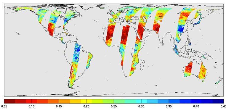
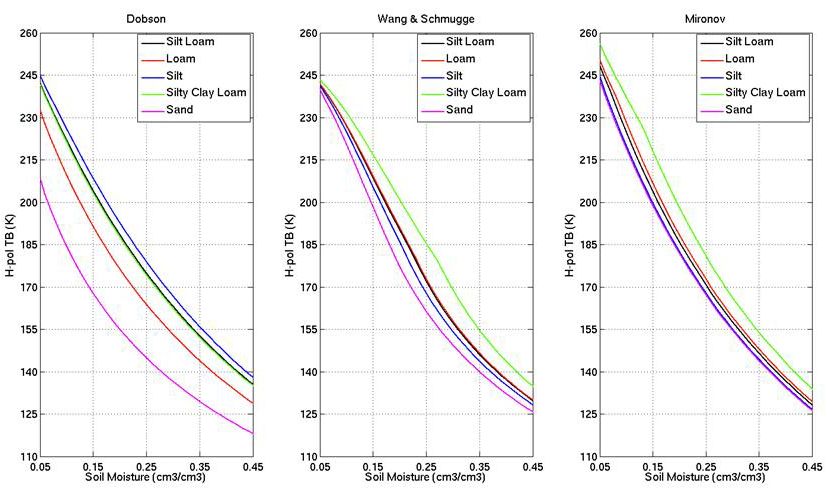
developed earlier; the resulting model not only applies to a wider range of soil types, but
also requires fewer input parameters – with clay percentage as the only soil input
parameter.
 These three models have been widely used due to their simple parameterizations and
applicability at L-band frequencies (1.26-1.41 GHz). As part of SMAP prelaunch and post-
launch calibration/validation activities, the performance of these dielectric models in terms
of bias and accuracy of the retrieved soil moisture was evaluated and a decision made on
which dielectric model to carry forward into the operational production of SMAP data
products. The SMAP L2_SM_P processing software has a switch which selects which
dielectric model will be used in the soil moisture retrieval. While all three dielectric models
are coded in the SMAP software, L2_SM_P currently uses the Mironov model in routine
processing. For comparison, ESA’s SMOS mission currently uses land cover classification
to choose the appropriate dielectric model (Dobson or Mironov). Figure 5 gives an
example of the performance of the three dielectric models when used in forward model
computations of L band TB for θ = 40°, assuming smooth bare soils at TS = 25°C for
different soil types.

 Figure 5. Bare soil TB as computed by different soil dielectric models. The selected soil types
 correspond to the top five most dominant soil texture classes, together accounting for
 over 80% of the global land area.

2.4 Use of the 6:00 AM Descending Node Orbit for the Primary Mission Product
 The decision to place SMAP into a sun-synchronous 6:00 am / 6:00 pm orbit is based
on a number of science issues relevant to the L2_SM_P product [24, 25]. Faraday rotation

 21
is a phenomenon in which the polarization vector of an electromagnetic wave rotates as the
wave propagates through the ionospheric plasma in the presence of the Earth's static
magnetic field. The phenomenon is a concern to SMAP because the polarization rotation
increases as the square of wavelength. If uncorrected, the SMAP polarized (H and V)
radiometer measurements will contain errors that translate to soil moisture error. Faraday
rotation varies greatly during the day, reaching a maximum during the afternoon and a
minimum in the pre-dawn hours. By using TB observations acquired near 6:00 am local
solar time as the primary input to the L2_SM_P product, the adverse impacts of Faraday
rotation are minimized. Faraday rotation correction to SMAP TB is described in the
L1B_TB ATBD.

 At 6:00 am the vertical profiles of soil temperature and soil dielectric properties are
likely to be more uniform [13] than at other times of the day (Figure 7). This early morning
condition will minimize the difference between canopy and soil temperatures and thermal
differences between land cover types within a pixel (Figure 6). These factors help to
minimize soil moisture retrieval errors originating from the use of a single effective
temperature to represent the near surface soil and canopy temperatures. This same
effective temperature can be used as the open water temperature in the water body
correction to TB that will be discussed in Sections 3 and 4.

 Figure 6. Schematic showing diurnal variation in temperature and thermal
 crossover times at approximately 6:00 am / 6:00 pm local time for
 various broad classes of land surface covers [modified from 24].

 22
(a)

 (b)

Figure 7. Soil temperature as a function of time based on June 2004 Oklahoma Mesonet data:
 (a) vertical profiles for a sod covered site and (b) the mean soil temperatures for
 bare soil (TB05, TB10) and sod (TS05, TS10). The shaded region identifies the
 period of the day when these effects result in less than 1° C difference among the
 four temperatures (T. Holmes, personal communication).

 Finally, it is desirable to establish a long-term climate data record of L-band brightness
temperatures and soil moisture. Such a data record could enable investigations of
important trends in emissivity, soil moisture, and other derived variables occurring over
annual to decadal periods. Both the SMOS and Aquarius L-band missions will operate in
6 am/6 pm orbits, and SMAP will extend these L-band data records.

 23
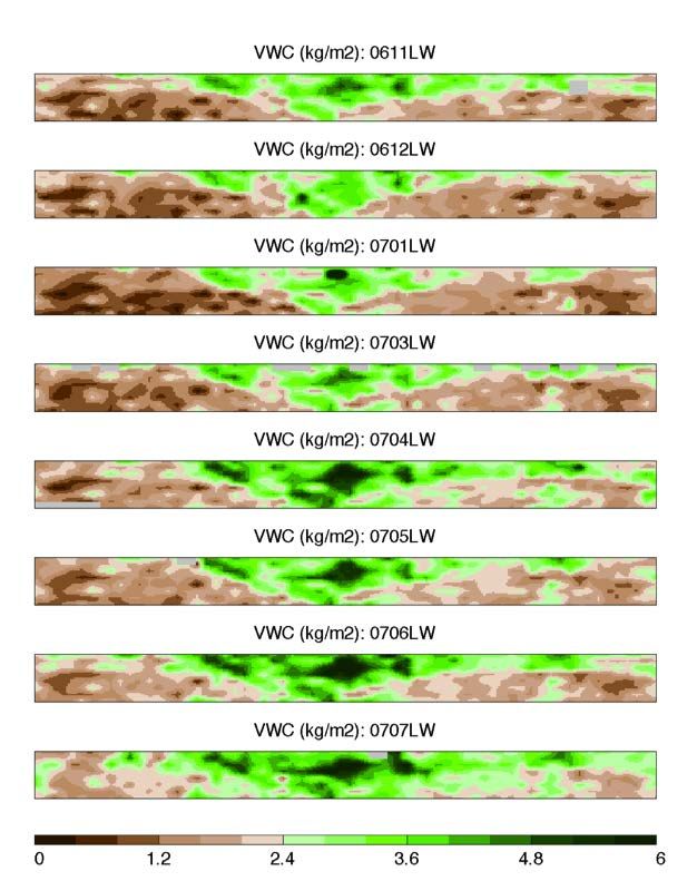
As will be discussed in Section 3, the current approach to generation of the baseline
L2_SM_P product was originally restricted to input data from the 6:00 am descending
passes because of the thermal equilibrium assumption and near-uniform thermal conditions
of surface soil layers and overlying vegetation in the early morning hours. Accurate soil
moisture retrievals using data from 6:00 pm ascending passes may require use of a land
surface model and will be generated as part of the L4_SM product (see ATBD for L4_SM).
However, some early results from the SMOS mission suggest that the additional error
associated with 6 pm retrievals may not be as large as expected [48]. As described in
Section 8.1, the SMAP project starting with L2_SM_P Data Release Version 4 (Dec., 2016)
produces a 6 pm retrieved soil moisture product using the same retrieval algorithm as the
6 am soil moisture product and with only very slightly degraded accuracy [61, 63].

3. PRODUCT OVERVIEW

 This ATBD covers the two coarse spatial resolution soil moisture products which are
based on the SMAP radiometer brightness temperatures: L2_SM_P, which is derived
surface soil moisture in half-orbit format at 40 km resolution output on a fixed 36-km
Equal-Area Scalable Earth-2 (EASE2) grid, and L3_SM_P, which is a daily global
composite of the L2_SM_P surface soil moisture, also at 40 km resolution output on a fixed
36-km EASE2 grid. Utilizing one or more of the soil moisture retrieval algorithms to be
discussed in section 4, SMAP brightness temperatures are converted into an estimate of the
0-5 cm surface soil moisture in units of cm3/cm3.

3.1 Inputs to Soil Moisture Retrieval

 The main input to the L2_SM_P processing algorithm is the SMAP L1C_TB product
that contains the time-ordered, geolocated, calibrated L1B_TB brightness temperatures
which have been resampled to the fixed 36-km EASE2 grid. In addition to general
geolocation and calibration, the L1B_TB data have also been corrected for atmospheric
effects, Faraday rotation, and low-level RFI effects prior to regridding. If the RFI
encountered is too large to be corrected, the TB data are flagged accordingly and no soil
moisture retrieval is attempted. See the L1B_TB and L1C_TB ATBDs for additional
details.

 In addition to TB observations, the L2_SM_P algorithm also requires ancillary datasets
for the soil moisture retrieval. These include:
 • Surface temperature
 • Vegetation opacity (or vegetation water content and vegetation opacity coefficient)
 • Vegetation single scattering albedo
 • Surface roughness information
 • Land cover type classification
 • Soil texture (sand, silt, and clay fraction)
 • Data flags for identification of land, water, precipitation, RFI, urban areas,
 mountainous terrain, permanent ice/snow, and dense vegetation

 24
The specific parameters and sources of these and other externally provided ancillary
data are listed in Section 6. Other parameters used by the L2_SM_P algorithm are
provided internally to the processing chain. These include a freeze/thaw flag, an open
water fraction, and a vegetation index; these were originally intended to be provided by the
SMAP radar L2_SM_A product (see L2_SM_A ATBD) or other ancillary sources. A
radiometer-based freeze/thaw flag is now being generated by the L3_FT_P team.

 All input TB and ancillary datasets used in the retrievals are mapped to the 36-km
EASE2 grid prior to entering the L2_SM_P processor. All input data, retrieved soil
moisture data, and flags utilize the same grid.

Figure 8. Conceptual list of input and output information for the L2_SM_P soil moisture product.

3.2 Algorithm Outputs
 Figure 8 lists in a conceptual way the variety of input and output data associated with
the SMAP L2_SM_P soil moisture product. Many of these parameters will be discussed
in Section 4 and Section 6. The primary contents of the output L2_SM_P and L3_SM_P
products are the retrieved soil moisture and associated quality control (QC) flags, as well
as the values of the ancillary parameters needed to retrieve the output soil moisture for that
grid cell. The exact Data Product Description for the L2_SM_P and L3_SM_P products
was generated in consultation with SMAP Science Data System (SDS) personnel, and is
available to the public through the NSIDC DAAC (see also Appendices 1 and 2).

 25
3.3 Product Granularity
 The L2_SM_P product is a half-orbit product. SMAP ascending (6 pm) half-orbits are
defined starting at the South Pole and ending at the North Pole, while descending (6 am)
half-orbits start at the North Pole and end at the South Pole. Input TB observations from a
given half-orbit are processed to generate output soil moisture retrievals for the same half
orbit.

 The L3_SM_P product is a daily product generated by compositing one day's worth of
L2_SM_P half-orbit granules, separately for ascending and descending half-orbits, onto a
global array. TB observations from descending (6 am) passes are used to retrieve soil
moisture for the L2_SM_P and L3_SM_P standard products as mentioned in Section 2.4.
Starting with L2_SM_P Data Release Version 4 in December, 2016, 6 pm soil moistures
are produced by applying the baseline 6 am retrieval algorithm to TB data from the 6 pm
ascending passes. The 6 pm soil moisture data will be done on a best effort basis and will
not be included in assessments of whether the L2_SM_P product meets the mission Level
1 requirements. However, the 6 pm retrievals will also be compared against observations
of soil moisture to assess their accuracy. Currently, the data volume estimate for the
L2_SM_P product is 15 MB/day and the data volume estimate for the L3_SM_P product
is 41 MB/day; these values are based on products from the 6 am descending pass only.

3.4 SMAP Product Suite
 The L2_SM_P and L3_SM_P products are part of the suite of SMAP products shown
previously in Table 2. The SMAP L1-L3 products will be generated by the SMAP Science
Data Processing System (SDS) at JPL, while the SMAP L4 products will be produced by
the Global Modeling and Assimilation Office (GMAO) at NASA GSFC. All SMAP data
products approved for release will be archived and made available to the public through a
NASA-designated Earth Science Data Center. NASA HQ has designated that the National
Snow and Ice Data Center (NSIDC) in Boulder, CO will be the primary SMAP DAAC,
although SMAP HiRes radar data will be archived separately at the Alaska Satellite Facility
(ASF) in Fairbanks, AK.

3.5 EASE Grid
 The grid selected for the SMAP geophysical (L2-L4) products is the updated Equal-
Area Scalable Earth-2 (EASE2) grid [26]. This grid was originally conceived at the NSIDC
and has been used to archive several satellite instrument data sets including SMMR, SSM/I,
and AMSR-E [27]. Using this same grid system for SMAP provides user convenience,
facilitates continuity of historical data grid formats, and enables re-use of heritage gridding
and extraction software tools developed for EASE grid.

 The EASE grid has a flexible formulation. By adjusting one scaling parameter it is
possible to generate a family of multi-resolution EASE grids that “nest” within one another.
The nesting can be made “perfect” in that smaller grid cells can be tessellated to form larger
grid cells, as shown in Figure. 9a. This feature provides SMAP data products with a
convenient common projection for both high-resolution radar observations and low-

 26
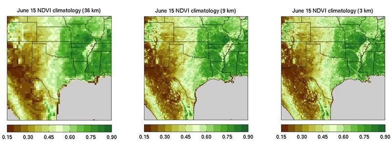
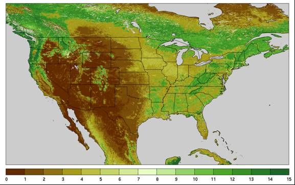
resolution radiometer observations. Figure 9b illustrates the different resolutions for the
3-, 9-, and 36-km EASE grids.

 A nominal EASE grid dimension of 36 km has been selected for the L2/3_SM_P
products. This is close to the 40-km resolution of the radiometer footprint and scales
conveniently with the 3 km and 9 km grid dimensions that have been selected for the radar-
only (L2/3_SM_A) and combined radar/radiometer (L2/3_SM_A/P) soil moisture
products, respectively. A global 36-km EASE grid can be constructed having an integer
number of rows and columns (408 and 963), with northernmost/southernmost latitudes of
±86.6225°, using a scaling parameter 1 that is almost exactly 36 km.

 36 km

 3 km

 9 km

 Figure 9a. Perfect nesting in EASE grid – smaller grid cells can be tessellated
 to form larger grid cells.

 Figure 9b. Example of ancillary NDVI climatology data displayed on the SMAP 36-km,
 9-km, and 3-km EASE grids.

1
 The precise value of the scaling parameter is 36.00040003 km at ±30° latitudes.

 27
You can also read