CLOUD-SCALE MOLECULAR GAS PROPERTIES IN 15 NEARBY GALAXIES
←
→
Page content transcription
If your browser does not render page correctly, please read the page content below
D RAFT VERSION M AY 4, 2018
                                                Typeset using LATEX twocolumn style in AASTeX61

                                                                        CLOUD-SCALE MOLECULAR GAS PROPERTIES IN 15 NEARBY GALAXIES

                                                            J IAYI S UN (孙嘉懿) , 1 A DAM K. L EROY , 1 A NDREAS S CHRUBA , 2 E RIK ROSOLOWSKY , 3 A NNIE H UGHES , 4, 5
                                                        J. M. D IEDERIK K RUIJSSEN , 6 S HARON M EIDT , 7 E VA S CHINNERER , 7 G UILLERMO A. B LANC , 8, 9 F RANK B IGIEL , 10
                                                   A LBERTO D. B OLATTO , 11 M ÉLANIE C HEVANCE , 6 B RENT G ROVES , 12 C INTHYA N. H ERRERA , 13 A LEXANDER P. S. H YGATE , 7, 6
                                                                      J ÉRÔME P ETY , 13, 14 M IGUEL Q UEREJETA , 15, 16 A NTONIO U SERO , 16 AND DYAS U TOMO 1
arXiv:1805.00937v1 [astro-ph.GA] 2 May 2018

                                              1 Department  of Astronomy, The Ohio State University, 140 West 18th Avenue, Columbus, OH 43210, USA
                                              2 Max-Planck-Institut für Extraterrestrische Physik, Giessenbachstraße 1, D-85748 Garching, Germany
                                              3 Department of Physics, University of Alberta, Edmonton, AB T6G 2E1, Canada
                                              4 CNRS, IRAP, 9 av. du Colonel Roche, BP 44346, F-31028 Toulouse cedex 4, France
                                              5 Université de Toulouse, UPS-OMP, IRAP, F-31028 Toulouse cedex 4, France

                                              6 Astronomisches Rechen-Institut, Zentrum für Astronomie der Universität Heidelberg, Mönchhofstraße 12-14, D-69120 Heidelberg, Germany
                                              7 Max-Planck-Institut    für Astronomie, Königstuhl 17, D-69117, Heidelberg, Germany
                                              8 Observatories    of the Carnegie Institution for Science, 813 Santa Barbara Street, Pasadena, CA 91101, USA
                                              9 Departamento de Astronomía, Universidad de Chile, Camino del Observatorio 1515, Las Condes, Santiago, Chile
                                              10 Institute für theoretische Astrophysik, Zentrum für Astronomie der Universität Heidelberg, Albert-Ueberle Str. 2, D-69120 Heidelberg, Germany
                                              11 Department of Astronomy, University of Maryland, College Park, MD 20742, USA

                                              12 Research School for Astronomy & Astrophysics Australian National University Canberra, ACT 2611, Australia
                                              13 Institut
                                                       de Radioastronomie Millimétrique (IRAM), 300 Rue de la Piscine, F-38406 Saint Martin d’Hères, France
                                              14 Observatoire de Paris, 61 Avenue de l’Observatoire, F-75014 Paris, France
                                              15 European Southern Observatory, Karl-Schwarzschild-Straße 2, D-85748 Garching, Germany
                                              16 Observatorio Astronómico Nacional (IGN),C/Alfonso XII, 3, E-28014 Madrid, Spain

                                                                                                              (Accepted 2018 Apr 26)

                                                                                                          ABSTRACT
                                                We measure the velocity dispersion, σ, and surface density, Σ, of the molecular gas in nearby galaxies from CO spectral line
                                              cubes with spatial resolution 45-120 pc, matched to the size of individual giant molecular clouds. Combining 11 galaxies from
                                              the PHANGS-ALMA survey with 4 targets from the literature, we characterize ∼ 30, 000 independent sightlines where CO is
                                              detected at good significance. Σ and σ show a strong positive correlation, with the best-fit power law slope close to the expected
                                              value for resolved, self-gravitating clouds. This indicates only weak variation in the virial parameter αvir ∝ σ 2 /Σ, which is ∼1.5-
                                              3.0 for most galaxies. We do, however, observe enormous variation in the internal turbulent pressure Pturb ∝ Σ σ 2 , which spans
                                              ∼5 dex across our sample. We find Σ, σ, and Pturb to be systematically larger in more massive galaxies. The same quantities
                                              appear enhanced in the central kpc of strongly barred galaxies relative to their disks. Based on sensitive maps of M31 and M33,
                                              the slope of the σ-Σ relation flattens at Σ . 10 M pc−2 , leading to high σ for a given Σ and high apparent αvir . This echoes
                                              results found in the Milky Way, and likely originates from a combination of lower beam filling factors and a stronger influence
                                              of local environment on the dynamical state of molecular gas in the low density regime.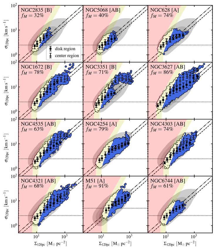
2                                                             S UN ET AL .

                    1. INTRODUCTION                                   bursts (Rosolowsky & Blitz 2005; Leroy et al. 2015), and one
   Observational evidence, including the close association of         lenticular galaxy (Utomo et al. 2015). In contrast, clouds sit-
H II regions with molecular clouds (see references in Morris          uated in regions with low gas density (e.g., the outer Galaxy;
& Rickard 1982) and the correlation between star formation            Heyer et al. 2001) or high ambient pressure (e.g., the Galactic
rate (SFR) tracers and molecular gas content (e.g., Rownd &           Center; Oka et al. 2001), tend to show much higher velocity
Young 1999; Wong & Blitz 2002; Bigiel et al. 2008; Schruba            dispersions than are expected for self-virialized clouds. This
et al. 2011), suggests that cold molecular gas is the direct gas      suggests that in these environments external gravitational po-
reservoir for star formation. On the other hand, the molec-           tential is at least as important as cloud self-gravity in regu-
ular interstellar medium (ISM) in galaxies is observed to             lating cloud dynamics (Heyer et al. 2009; Field et al. 2011;
have diverse physical properties and dynamical states (e.g.,          Kruijssen et al. 2014).
Elmegreen 1989). Within a galaxy and even within an in-                  Despite the insight obtained by these Galactic and early
dividual cloud, molecular gas can show a range of surface             extragalactic studies, our knowledge of the physical state of
and volume densities, turbulent velocities, and bulk motions.         molecular gas in other galaxies remains limited. Many extra-
For a thorough understanding of how star formation happens            galactic molecular cloud studies target Local Group galaxies
in galaxies, it is critical to know how galactic environments         and the nearest dwarf galaxies (Rosolowsky 2007; Bolatto
(e.g., large-scale gas dynamics and stellar feedback) influ-          et al. 2008; Wong et al. 2011; Druard et al. 2014). Although
ence the physical properties of the molecular gas, and how            nearby, these systems are not representative of where most
the gas properties in turn determine its ability to form stars.       stars in the present-day Universe form. Low mass galaxies
   The evolution of a molecular cloud depends primarily on            tend to show faint, isolated CO emission (Fukui et al. 1999;
the balance between its kinetic and gravitational potential           Engargiola et al. 2003; Schruba et al. 2017), distinct from the
energy. Other mechanisms, e.g., magnetic fields and exter-            bright, spatially contiguous emission distributions observed
nal pressure, might also act to support or confine the cloud.         in more massive galaxies (Hughes et al. 2013a). As inter-
In both observational and theoretical work, this balance is           ferometers force trade-offs between surface brightness sen-
commonly described by the virial parameter, αvir ≡ 2K/Ug ,            sitivity and resolution, it remains challenging to access the
which captures the ratio between kinetic energy, K, and               entire cloud population of normal star-forming disk galax-
self-gravitational potential energy, Ug . Theoretical work            ies, (which are usually & 10 times more distant than Local
by McKee & Zweibel (1992); Krumholz & McKee (2005);                   Group targets), with most contemporary observing facilities.
Padoan & Nordlund (2011); Federrath & Klessen (2012);                 Most studies to date have either focused on a single galaxy
Kruijssen (2012); Krumholz et al. (2012); Hennebelle &                (Colombo et al. 2014a; Egusa et al. 2018; Faesi et al. 2018)
Chabrier (2013); Padoan et al. (2017) predict that αvir plays         or on the most massive clouds in the inner regions of a small
an important role in determining the ability of a cloud to form       sample of galaxies (Donovan Meyer et al. 2013).
stars and stellar clusters. In these theories, clouds with high          In this paper, we take the logical next step, exploring the
αvir (i.e., a relative excess of kinetic energy) form fewer stars     surface density, line width, and dynamical state of molecular
per unit time for a given gas mass and density. As a result,          gas across a significant sample of star-forming disk galaxies.
the dynamical state of molecular gas at the scale of individ-         This is made possible by the ongoing PHANGS-ALMA sur-
ual molecular clouds represents an important consideration            vey (PHANGS-ALMA: Physics at High Angular-resolution
for galactic-scale theories and simulations of star formation.        in Nearby GalaxieS with ALMA, A. K. Leroy et al. 2018,
   On the observational side, this topic has been investigated        in prep.; ALMA: Atacama Large Millimeter-submillimeter
via studies of individual clouds both in the Galaxy and sev-          Array). PHANGS-ALMA is mapping the CO (2-1) emission
eral nearby galaxies. Most commonly, analysis of the CO               from a large sample of nearby star-forming galaxies (74 in to-
line emission from the molecular medium provides estimates            tal) with sufficient sensitivity and resolution to detect individ-
of the cloud velocity dispersion, σ, surface density, Σ, size,        ual giant molecular clouds (GMCs) across most of the galax-
R, and mass, M. The relationship between these quantities             ies’ star-forming disks. In this paper, we combine the first
then gives information about the physical state of the cloud          11 galaxies from PHANGS-ALMA with four targets (M31,
(following Larson 1981).                                              M33, M51, and the Antennae Galaxies) previously observed
   Recent work on this topic tends to emphasize the relation-         at high spatial resolution. These 15 galaxies span dwarf spi-
ship between σ 2 /R and Σ (e.g., Heyer et al. 2009; Leroy             rals to starburst galaxies, and yield tens of thousands inde-
et al. 2015), as the position of a cloud in σ 2 /R-Σ space            pendent measurements at spatial scales of 20 − 130 pc, com-
probes its dynamical state and internal gas pressure (Keto            parable to the characteristic size of a GMC.
& Myers 1986; Field et al. 2011). A nearly linear scaling                We present more details about our dataset in Section 2, and
relation between σ 2 /R and Σ, suggestive of bound clouds             explain the measurements that we perform in Section 3. In
with velocity dispersion balancing their self-gravity, has been       Section 4 we discuss expectations for the σ-Σ scaling rela-
observed for clouds in the Milky Way disk (Heyer et al.               tion based on simple theoretical arguments. In Section 5,
2009), the Large Magellanic Cloud (LMC; Wong et al. 2011),            we present the empirical scaling relation that best describes
nearby dwarf galaxies (Bolatto et al. 2008), spiral galaxies          the relationship between line width and surface density for
(Donovan Meyer et al. 2013; Colombo et al. 2014a), star-              our sample of nearby galaxies. Then, in Section 6 we dis-
                                                                      cuss their physical interpretation. We present a summary of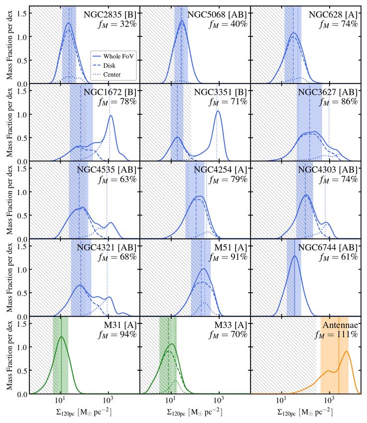
C LOUD -S CALE M OLECULAR G AS P ROPERTIES IN 15 N EARBY G ALAXIES                                    3

our main results in Section 7, along with prospects for future   et al. 2017). As a result, we expect individual molecular
work.                                                            clouds to be at least marginally resolved in these maps.
                                                                    The channel width for most of these observations is 2.5-
                                                                 2.6 km s−1 . The two exceptions are the Antennae and M51,
                          2. DATA                                which have 5.0 km s−1 channel width. This velocity resolu-
   Our sample consists of 15 nearby galaxies with high reso-     tion should be sufficient to measure the velocity dispersion
lution maps of low-J carbon monoxide (CO) rotational line        for larger GMCs, but may bias the measurement to higher
emission. Table 1 lists their name, morphology, orienta-         values for smaller GMCs. We account for the effect of finite
tion, adopted distance and stellar mass for each galaxy and      channel width in our analysis and discuss its implications in
the basic parameters of the CO data. Our sample includes         Section 3.4. We note that both M51 and the Antennae are
11 targets from the PHANGS-ALMA survey (A. K. Leroy              gas-rich, and typically have high line widths (Colombo et al.
et al. 2018, in prep.). These targets were observed by           2014a; Whitmore et al. 2014).
ALMA in CO (2-1) using the 12-meter and 7-meter inter-              In Table 1, we also quote the sensitivity (1σ channel-
ferometric arrays as well as the total-power antennas. Thus,     wise rms noise) of each data cube in units of K at their na-
the maps capture information from all spatial scales. The        tive angular resolution before any convolution. For objects
whole PHANGS-ALMA sample is designed to cover the                in the PHANGS-ALMA survey, the sensitivity of velocity-
star-forming main sequence of galaxies across the local vol-     integrated intensity maps are typically ∼0.5 K km s−1 , cor-
ume. When finished, it will provide ∼ 1-1.500 resolution         responding to a gas surface density of 3 M pc−2 for our
CO (2-1) maps of 74 nearby (d . 17 Mpc), ALMA-visible,           assumed CO-to-H2 conversion factor and CO line ratios (see
actively star-forming galaxies down to a stellar mass of ∼       Section 3.3). This surface brightness sensitivity improves as
5 × 10⁹ M . A detailed description of the PHANGS-ALMA            we convolve our data cubes to coarser angular resolutions to
sample, observing strategy and data reduction is presented in    achieve uniform linear resolution across our targets.
A. K. Leroy et al. (2018, in prep.).                                We provide additional notes on a few galaxies in our sam-
   Observations of the full PHANGS-ALMA sample are cur-          ple:
rently underway, but the first 11 targets analyzed here were
                                                                     • NGC 2835: a low mass star-forming disk galaxy. The
already observed in 2016 during ALMA’s Cycle 3. These tar-
                                                                       CO map has relatively low sensitivity due to the ex-
gets sparsely sample the star-forming main sequence with an
                                                                       tended interferometer configuration used during the
emphasis on higher mass systems.
                                                                       observations. Furthermore, the CO surface brightness
   To supplement these first PHANGS-ALMA targets, we in-
                                                                       is low in accordance with the galaxy’s low stellar mass.
clude the PdBI Arcsecond Whirlpool Survey (PAWS) CO (1-
0) map of M51 (Pety et al. 2013; Schinnerer et al. 2013),            • NGC 3351: a strongly barred galaxy with a prominent
which incorporates short-spacing data from the IRAM 30-m               central molecular gas disk (Jogee et al. 2005), a gas-
telescope. M51 is a massive grand-design spiral on the star-           poor bulge, and a ring of molecular gas at larger galac-
forming main sequence.                                                 tocentric radius. Star formation takes place both in the
   We also analyze the Local Group galaxies M31 and M33.               central disk and in the molecular gas ring outside the
For M31, we use the CARMA CO (1-0) survey by A.                        bulge.
Schruba et al. (in prep.), which includes short- and zero-
spacing data from the IRAM 30-m telescope (Nieten et al.             • NGC 5068: a low mass star-forming disk galaxy. Sim-
2006). For M33, we use the IRAM 30-m CO (2-1) survey by                ilar to NGC 2835, the sensitivity of the CO map for
Gratier et al. (2010) and Druard et al. (2014). M31 and M33            this target is lower than for our other targets.
extend the parameter space probed by our galaxy sample
down to low gas surface density regimes (see Section 5.2.4).         • NGC 6744: a weakly barred star-forming spiral galaxy.
   Finally, we include the ALMA CO (3-2) map of the inter-             The PHANGS-ALMA CO map covers the north and
acting region of the Antennae galaxies presented by Whit-              south part of the disk, but has no coverage of the (gas-
more et al. (2014), and analyzed by Johnson et al. (2015)              poor) center.
and Leroy et al. (2016). The physical state of the gas in the        • M51: a normal star-forming disk galaxy with grand-
Antennae may be strongly affected by the galaxy merger; we             design spiral structure. The PAWS CO map covers the
include this CO map here as a point of contrast to the normal,         central 9 × 6 kpc2 region (see Schinnerer et al. 2013).
undisturbed disk galaxies targeted by PHANGS-ALMA.
   This combination of PHANGS-ALMA and literature data               • M31: this high stellar mass Local Group spiral is
gives us (by far) the largest sample of star-forming galax-            a “green valley” galaxy (i.e., it is located between
ies with cloud-scale-resolution CO maps, and the prospect              the “blue cloud” and the “red sequence” in a color-
to expand this analysis to ∼80 galaxies in the near future is          magnitude diagram, see e.g., Figure 4 of Mutch et al.
clearly exciting. The angular resolution of these maps (see            2011, for an illustration), with relatively quiescent star
Table 1) corresponds to linear scales of 20-130 pc. These res-         formation (e.g., Lewis et al. 2015). The CARMA
olutions are comparable to the typical size of Galactic GMCs           CO survey covers the north-eastern part of the star-
(Solomon et al. 1987; Heyer et al. 2009; Miville-Deschênes             forming ring and a part of the inner disk (A. Schruba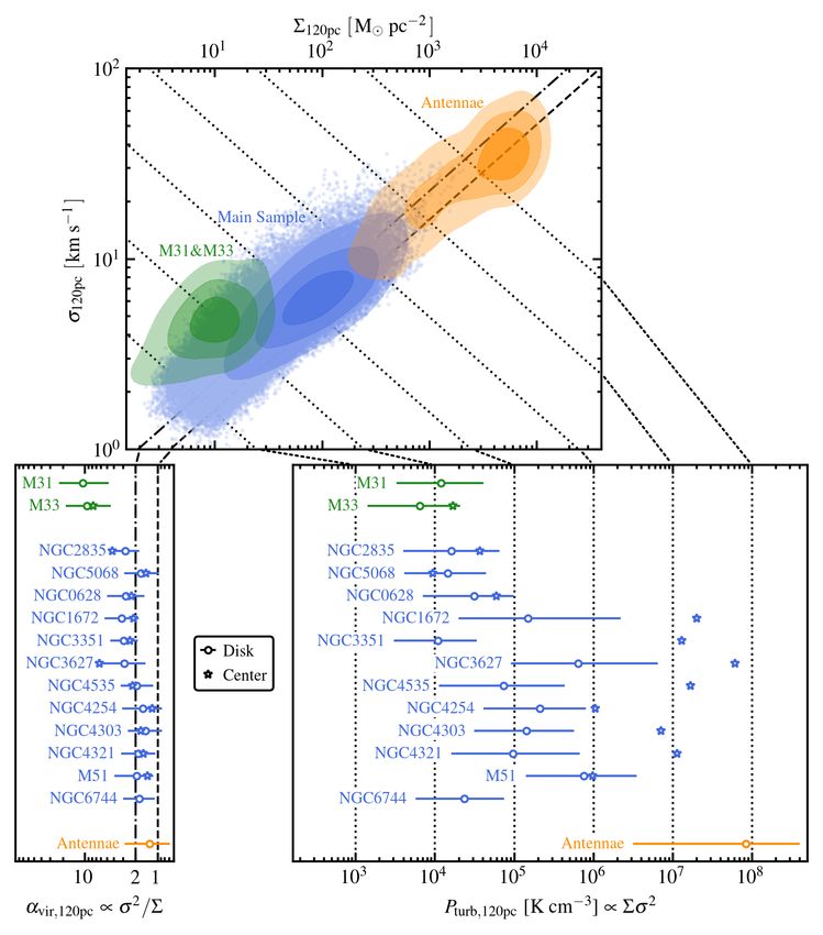
4                                                                         S UN ET AL .

                                                                Table 1. Sample of Galaxies

        Galaxy      Morphology      Distancea    Inclinationb    Stellar Massc   Telescope        Line     Resolution   Channel Width      Sensitivity
                                      [Mpc]          [◦ ]         [1010 M ]                                 [00 / pc]       [km s−1 ]         [K]

      NGC 628           Sc-A           9.0           6.5              2.1          ALMA          CO(2-1)    1.0 / 44          2.5             0.13
      NGC 1672          Sb-B           11.9          40.0             3.0          ALMA          CO(2-1)    1.7 / 98          2.5             0.09
      NGC 2835          Sc-B           10.1          56.4            0.76          ALMA          CO(2-1)    0.7 / 34          2.5             0.27
      NGC 3351          Sb-B           10.0          41.0             3.2          ALMA          CO(2-1)    1.3 / 63          2.5             0.12
      NGC 3627         Sb-AB           8.28          62.0             3.6          ALMA          CO(2-1)    1.3 / 52          2.5             0.09
      NGC 4254          Sc-A           16.8          27.0             6.5          ALMA          CO(2-1)    1.6 / 130         2.5             0.06
      NGC 4303        Sbc-AB           17.6          25.0             7.4          ALMA          CO(2-1)    1.5 / 128         2.5             0.10
      NGC 4321        Sbc-AB           15.2          27.0             7.9          ALMA          CO(2-1)    1.4 / 103         2.5             0.09
      NGC 4535         Sc-AB           15.8          40.0             3.9          ALMA          CO(2-1)    1.5 / 115         2.5             0.08
      NGC 5068        Scd-AB           9.0           26.9             1.1          ALMA          CO(2-1)    0.9 / 39          2.5             0.24
      NGC 6744        Sbc-AB           11.6          40.0             8.1          ALMA          CO(2-1)    1.0 / 56          2.5             0.18
      M51              Sbc-A           8.39          21.0             7.7           PdBI         CO(1-0)    1.2 / 49          5.0             0.31
      M31               Sb-A           0.79          77.7             16          CARMA          CO(1-0)    5.5 / 21          2.5             0.19
      M33              Scd-A           0.92          58.0           0.3-0.6      IRAM-30m        CO(2-1)    12 / 54           2.6             0.04
      Antennae         Merger          22.0           –               –            ALMA          CO(3-2)    0.6 / 64          5.0             0.13
     a Distance values are taken from the Extragalactic Distance Database (Tully et al. 2009).
     b References for the inclination angle values: NGC 628 - Fathi et al. (2007); NGC 1672 - Díaz et al. (1999); NGC 2835 & 5068 - values from
       the HyperLeda database (Makarov et al. 2014); NGC 3351 - Dicaire et al. (2008); NGC 3627 - de Blok et al. (2008); NGC 4254, 4321, 4535 -
       Guhathakurta et al. (1988); NGC 4303 - Schinnerer et al. (2002); NGC 6744 - Ryder et al. (1999); M51 - Colombo et al. (2014b); M31 - Corbelli
       et al. (2010); M33 - E. Koch et al. (2018, in prep.).
     c References for the stellar mass values: NGC 2835 & 6744 - A. K. Leroy et al. (2018, in prep.); M31 - Barmby et al. (2006); M33 - Corbelli (2003);
       all other galaxies - S4 G global stellar masses (Spitzer Survey of Stellar Structure in Galaxies; Sheth et al. 2010; Querejeta et al. 2015).

      et al. in prep.; and see visualizations in Caldú-Primo                       locity dispersion, σ, along each sightline at a range of fixed
      & Schruba 2016; Leroy et al. 2016). Because of its                           spatial scales. This approach has been advocated by Leroy
      proximity (d ∼ 0.79 Mpc, Tully et al. 2009), the sensi-                      et al. (2016) based on earlier work by Ossenkopf & Mac
      tivity of the CO data for this target is much better than                    Low (2002), Sawada et al. (2012), Hughes et al. (2013b),
      for most other galaxies in our sample. The gas reser-                        and Leroy et al. (2013). Recent work analyzing high resolu-
      voir in M31 is dominated by the large H I disk (Braun                        tion and high sensitivity ALMA data has also adopted similar
      et al. 2009), and most of its molecular gas content sits                     approaches (e.g., Egusa et al. 2018).
      at relatively large galactic radius.                                            This approach gives us access to all essential physical
                                                                                   properties that we would like to measure (e.g., gas sur-
    • M33: this low stellar mass Local Group dwarf spiral                          face density, velocity dispersion, dynamical state, and tur-
      is also H I-dominated (see Druard et al. 2014). Again,                       bulent energy content). Such “fixed-spatial-scale” (or sim-
      due to its proximity (d ∼0.92 Mpc, Tully et al. 2009),                       ply “fixed-scale”) approach is non-parametric, minimal in as-
      the sensitivity and spatial resolution of the CO data for                    sumptions, and easy to apply to many data sets in a uniform
      M33 are better than for most of our sample.                                  way. Our measurements are easy to replicate in synthetic
                                                                                   observations, and thus offer a straightforward path for direct
    • The Antennae Galaxies: the nearest major merger. The
                                                                                   comparison between observations and simulations. Finally,
      CO map presented in Whitmore et al. (2014) covers
                                                                                   this apporach characterizes all detected CO emission, and al-
      only the interacting (“overlap”) region. This is the only
                                                                                   lows us to rigorously treat the selection function.
      target in our sample that lacks short- and zero-spacing
                                                                                      Our fixed-scale approach differs from the cloud iden-
      data.
                                                                                   tification approaches commonly used in previous studies
                     3. MEASUREMENTS                                               (e.g., Clumpfind, see Williams et al. 1994; cprops, see
                                                                                   Rosolowsky & Leroy 2006). These methods segment CO
     3.1. Fixed-Spatial-Scale Measurement Approach                                 emission by associating CO emission with local maxima.
   From the high resolution CO imaging described in Section                        While this is a useful strategy for identifying isolated struc-
2, we estimate the molecular gas surface density, Σ, and ve-                       tures, there are three overlaping drawbacks that makes us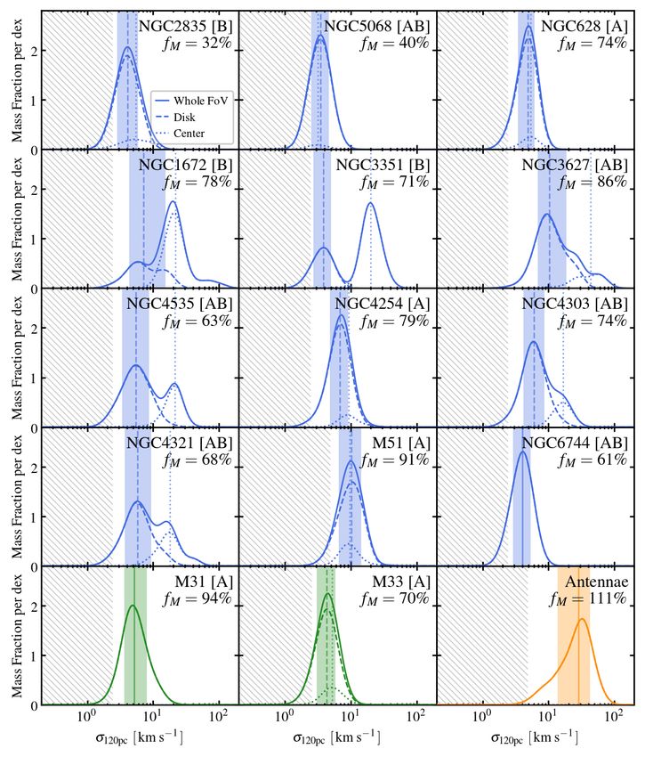
C LOUD -S CALE M OLECULAR G AS P ROPERTIES IN 15 N EARBY G ALAXIES                                            5

prefer the fixed-scale approach. First, the criteria for seg-                  first identify all 3D regions in the data cube where ≥ 2 con-
mentation are usually not physically motivated. Instead, sev-                  secutive channels show emission with signal-to-noise ratio
eral recent studies (Pineda et al. 2009; Hughes et al. 2013a;                  (S/N) ≥ 5. Then, we expand this mask in both spatial and
Leroy et al. 2016) have shown that cloud identification meth-                  spectral directions to include all adjacent pixels that contain
ods tend to find beam-sized objects when applied to data                       CO emission in ≥ 2 consecutive channels with S/N ≥ 2. This
sets with moderate resolution and sensitivity. Second, at                      signal identification scheme is similar to those adopted in
45–120 pc resolution, we observe many crowded regions                          other works (e.g., cprops, see Rosolowsky & Leroy 2006).
since we target the molecular gas rich parts of star-forming                      Note that for most of our targets, we detect CO emission at
galaxies (e.g., galaxy centers, spiral arms, and bar ends). The                relatively high S/N and much of the emission is spatially con-
commonly used segmentation algorithms are not optimized                        nected. In these cases, our sensitivity limit mostly reduces to
for identifying marginally resolved clouds in this regime.                     the 2-consecutive-2σ-channels criterion. However, our two
Third, some segmentation algorithms do not characterize all                    low stellar mass PHANGS-ALMA galaxies, NGC 2835 and
emissions, which then makes the selection function complex.                    NGC 5068, have lower overall S/N. For these targets, the
Based on all these, we believe that the fixed-scale approach is                2-consecutive-5σ-channel criterion becomes more relevant.
at least as appropriate in this context as cloud identification.               We project the selection effects due to these limits into the
   Our fixed-scale approach does not provide information on                    key parameter space that we study (Section 5.2).
the spatial extent of the CO emitting structures. For the rest                    Faint line wings extending to velocities far from the cen-
of this study, we adopt the spatial resolution of the data to be               troid can have an important effect on the line width. With this
the relevant size scale when, e.g., estimating the mean vol-                   in mind, we expand the mask along the velocity axis to cover
ume density and virial parameter. We expect this to be a rea-                  the entire probable velocity range of the CO line. The amount
sonable assumption as long as two conditions hold: (1) the                     by which we grow the mask depends on the ratio between
beam size is within the scale-free range of the hierarchical                   the intensity at the line peak and at the edge of the mask, and
molecular ISM (often taken to be either the disk scale height                  hence varies between sightlines. Based on the peak-to-edge
or the turbulent driving scale, and typically about a hundred                  ratio, we expand the mask so that it would extend to ±3σ if
or a few hundreds of parsec, see e.g., Brunt 2003) and (2)                     the line profile has a Gaussian shape with our measured peak
bright CO emission fills a large fraction of the beam. When                    intensity centered at the peak velocity.
condition (2) is violated, the beam-averaged surface density                      For each sightline in the mask, we calculate the line-
is diluted by the “dark area” and we no longer expect the                      integrated intensity ICO and peak intensity Tpeak of the emis-
beam size to represent the relevant size scale (i.e., beam dilu-               sion within the expanded mask. We further convert these CO
tion, see Section 4). Nevertheless, this concern is not specific               line measurements into the molecular gas surface density Σ
to the fixed-scale approach, but generally applicable to most                  and velocity dispersion σ following the procedures described
analysis using data sets with moderate spatial resolution.                     in the next two sections (Section 3.3 and 3.4).
   The sampling scale is an adjustable variable in the fixed-                     For the line-integrated intensity, peak intensity, and all
scale approach. We explore the impact of using different                       other measurements, we estimate their statistical errors by
sampling scales by changing the linear resolution of the data                  performing a Monte Carlo simulation using the data cube it-
(see Section 3.2), and repeat our measurements at each reso-                   self as model. We generate 1, 000 realizations of the data
lution. This lets us investigate molecular gas properties as a                 cube by artificially adding random noise to the original cube,
function of averaging scale.                                                   and repeat all our measurements for each realization. Note
                                                                               that the mask is only generated once for each galaxy using
                   3.2. Measurement Procedure
                                                                               the original cube, and then it is applied to all the 1, 000 mock
  Before performing any measurements, we pre-process all                       cubes. We record the rms scatter of the repeated measure-
data sets by convolving them to a set of round Gaussian-                       ments and quote these numbers as the statistical uncertain-
shaped beams with fixed linear sizes: 45, 60, 80, 100, and                     ties.
120 pc (at FWHM). When the native angular resolution of
a data set is coarser than the target beam size, we exclude                                        3.3. Surface Density
that galaxy from the analysis at that spatial scale1 . Then, at
each resolution, we resample the data sets onto regular square                   We estimate a surface density, Σ, from the line-integrated
grids so that the pixels Nyquist-sample the new beam, result-                  CO intensity, ICO , along each detected sightline. Through-
ing in an (areal) over-sampling factor of π/ ln 2 ≈ 4.53.                      out the paper, we assume that the low-J CO lines trace mass
  In each data set and at each resolution, we identify all                     in a simple way, so that we can estimate Σ from ICO and
sightlines2 with significant CO emission. To do this, we                       an adopted CO-to-H2 conversion factor (Bolatto et al. 2013).
                                                                               We adopt the following conversion factors αCO ≡ Σ/ICO :

   1 In practice, due to the uncertainty in the distances to our targets, we
allow a 10% tolerance so that a target with its native resolution between 72              αCO(1−0) = 4.35 M pc−2 (K km s−1 )−1 ,           (1)
and 88 pc will be labeled as 80 pc.
   2 We use the word “sightline” to denote the Nyquist-sampled pixels                     αCO(2−1) = 6.25 M pc−2 (K km s−1 )−1 ,           (2)
throughout this paper.                                                                    αCO(3−2) = 17.4 M pc−2 (K km s−1 )−1 .           (3)
6                                                           S UN ET AL .

These correspond to the Galactic value for CO (1-0) recom-            For our main results, we use the “effective width”3 as a
mended by Bolatto et al. (2013) along with transition line ra-      proxy for the line width. Following Heyer et al. (2001), we
tios of CO (2-1)/CO (1-0)=0.7 (Leroy et al. 2013; Saintonge         define the effective width as
et al. 2017) and CO (3-2)/CO (1-0)=0.25 for the Antennae
(Ueda et al. 2012; Bigiel et al. 2015). These take the contri-                                                 ICO
                                                                                            σ measured = √             ,                       (4)
bution from helium and other heavy elements into account.                                                     2π Tpeak
   A single conversion factor has the merit of showing our
measurements directly, but we have good reason to believe           where Tpeak is the specific intensity at the line peak (in K).
that αCO varies across our sample (Blanc et al. 2013; Sand-         This proxy is less sensitive to noise in line wings than the
strom et al. 2013). Despite a general understanding of the          second moment and, unlike direct profile fitting, it does not a
likely variations in αCO (Bolatto et al. 2013), we still lack       priori assume any particular line shape. However, the effec-
a quantitative, observationally verified prescription for αCO       tive width can be sensitive to the channel width.
that applies at cloud scales. Moreover, cloud scale mod-               To correct for the broadening caused by finite channel
els of the CO-to-H2 conversion factor often identify the line       width and spectral response curve width, we subtract the ef-
width of a cloud and/or its density as an important quantity        fective width of the spectral response from the measured ef-
(Maloney & Black 1988; Narayanan et al. 2012). Thus our             fective width (Rosolowsky & Leroy 2006):
measurements may have a complicated, non-linear interac-                                  q
tion with αCO . We adopt a single αCO and then discuss pos-                           σ = σ 2measured − σ 2response ,           (5)
sible variations when they become relevant. A more general
exploration of αCO for the CO (2-1) line is a broad goal of         where σ response is estimated from the channel width and the
the PHANGS-ALMA science program.                                    channel-to-channel correlation coefficient, following Leroy
   As most of the galaxies in our sample have relatively high       et al. (2016). Appendix B presents the detailed procedures
metallicity and PHANGS-ALMA targets their molecular-                for estimating σ response , as well as discussions on the applica-
gas-rich inner regions, we expect most of the molecular gas         bility of this “deconvolution-in-quadrature” approach. This
to produce bright CO emission. That is, “CO-dark” molecu-           broadening correction should be accurate enough in most
lar gas should not represent a dominant fraction of the molec-      cases, except when the measured line width becomes close
ular gas mass, and the CO line width should be representa-          to the channel width. In the following sections, we indicate
tive of the true H2 velocity dispersion. We do include some         this regime in our plots and discuss resolution effects, if rel-
low mass spiral galaxies in our analysis (M33, NGC 2835,            evant, when presenting our results.
NGC 5068) and here the contributions of a CO-dark phase                One important caveat related to the line width near the cen-
may be more significant (though αCO likely varies by less           ters of galaxies is that we do not correct for unresolved rota-
than a factor of 2, see Gratier et al. 2017).                       tional motions or contributions from multiple clouds along
   We assume that our spatial resolution is sufficient to reach     the line of sight. This “beam smearing” effect may be impor-
the scale of individual GMCs or small collections of GMCs,          tant where the rotation curve rises quickly, even at our high
and we take such structures to be spherically symmetric.            resolution. The ongoing efforts of measuring rotation curves
Therefore, we do not apply any correction to Σ to account           from PHANGS-ALMA data (P. Lang et al. in preparation)
for beam filling factors or the effect of galaxy disk inclina-      will allow a more careful treatment of this effect in the fu-
tion.                                                               ture.

                                                                                               3.5. Completeness
                                                                      Table 2 reports the number of independent measurements
                                                                    and total emission within the mask, expressed as molecular
                                                                    gas mass, in each target at 45, 80, and 120 pc resolution. In
                       3.4. Line Width                              massive disk galaxies, thousands of independent sightlines
   We use the width of the CO emission line to trace the ve-        show CO emission above our sensitivity limit. This number
locity dispersion, σ, of molecular gas along each sightline.        drops to hundreds in our lower mass targets. For our adopted
For the most part, we expect that the CO line width is driven       CO-to-H2 conversion factor, the molecular mass implied by
by turbulent broadening, and thus it directly traces the tur-       the CO flux along each sightline is ∼ 104 − 106 M , and the
bulent velocity dispersion at the spatial scale set by the data     implied surface density is ∼ 10 − 103 M pc−2 .
resolution.                                                           In total, our detected sightlines include CO emission equiv-
   Several methods exist to estimate the width of an emission       alent to 107 − 109 M of molecular gas per galaxy. Some
line. Common approaches include fitting the line profiles
with a Gaussian function or Hermite polynomials, calculat-             3 Heyer et al. (2001) and following works refer to this quantity as “equiv-
ing the second moment (i.e., the rms dispersion of the spec-        alent width”. We notice that this name has different meaning in other con-
trum), or measuring an “effective width” (see below). These         texts (e.g., it is also defined as the ratio between the total flux of an emis-
methods have varying levels of robustness against noise and         sion/absorption line and the underlying continuum flux density). We instead
make different assumptions about the shape of the line.             adopt the name “effective width” here to avoid confusions in terminology.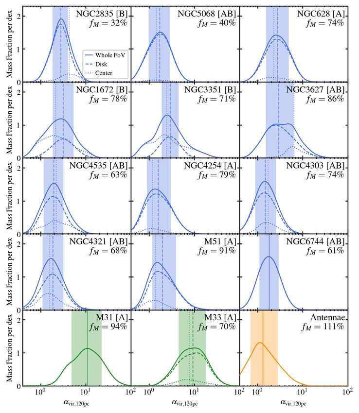
C LOUD -S CALE M OLECULAR G AS P ROPERTIES IN 15 N EARBY G ALAXIES                                                         7

                                                               Table 2. CO Detection Statistics

                     Galaxy              at 45 pc resolution                  at 80 pc resolution                at 120 pc resolution

                                 Nsightlines      Mmol          fM   Nsightlines     Mmol           fM    Nsightlines     Mmol          fM
                                               [108   M ]                          [108   M ]                           [108   M ]

                   NGC 2835         408           0.45         26%      308           0.59          33%      183          0.58          32%
                   NGC 5068         914            1.1         32%      637           1.4           40%      370           1.4          40%
                   NGC 628         6,156           6.7         45%     4,307          8.9           66%     2,711          10           74%
                   NGC 1672          –                –         –        –                –          –      1,239          21           78%
                   NGC 3351          –                –         –      1,180          5.7           63%      990           6.4          71%
                   NGC 3627          –                –         –      4,030           28           84%     2,185          28           86%
                   NGC 4535          –                –         –        –                –          –      2,031          18           63%
                   NGC 4254          –                –         –        –                –          –      5,485          62           79%
                   NGC 4303          –                –         –        –                –          –      3,522          44           74%
                   NGC 4321          –                –         –        –                –          –      4,432          47           68%
                   M51             6,087           28          80%     2,656           29           87%     1,484          31           91%
                   NGC 6744          –                –         –      3,353          8.7           52%     2,351          10           61%
                   M31             2,266          0.68         66%     1,384          0.88          86%      780          0.96          94%
                   M33               –                –         –      1,798          1.0           63%     1,147          1.1          70%
                   Antennae          –                –         –      1,097           62       111%†        603           62        111%†

                  N OTE—For each galaxy at each resolution level, we report: (1) Nsightlines - number of independent sightlines with
                    confident CO detection (i.e., the number of all CO-detected sightlines divided by the areal over-sampling factor
                    4.53); (2) Mmol - total recovered molecular gas mass (in units of 108 M ); and (3) fM - fraction of the recovered gas
                    mass comparing to the total gas mass inside the same field of view.
                    Galaxies are ordered following such scheme: the 12 galaxies in our “main sample” (PHANGS-ALMA targets plus
                    M51) appear first, among which the ordering is determined by increasing total stellar mass (see Table 1); then the
                    Local Group objects and the Antennae galaxies follow.
                  † The derived fraction of recovered gas mass exceeds 100% in the Antennae galaxies because the data cubes lack
                    short-spacing information and thus exhibit “clean bowls”. These features show up as large regions with unphysical
                    negative signals adjacent to bright emission structures. Summing over these negative signals reduces the estimated
                    total gas mass (see also Leroy et al. 2016).

emission remains outside the mask, however, as it is too faint                                                 4. EXPECTATIONS
to be detected at good significance using our CO emission                                           4.1. Expectations about Cloud Properties
identification method. We estimate the fraction of the CO
flux included in our analysis, fM , by dividing the total flux                           In early studies of the Milky Way cloud population (e.g.,
inside the mask by the sum of the unmasked cube. Because                              Solomon et al. 1987), GMCs are usually assumed to be
most of our data cubes (all but the Antennae galaxies) incor-                         long-lived, roughly virialized structures. Departures from
porate total power data, and most targets have strong enough                          virial equilibrium can be expressed via the virial parame-
CO emission, we expect a direct sum of the cube to yield a                            ter, αvir ≡ 2K/Ug , where K and Ug denote the kinetic en-
robust estimate of the total flux.                                                    ergy and self-gravitational potential energy. Virialized clouds
   We report fM for each data set at each resolution in Table 2.                      without surface pressure or magnetic support have αvir = 1,
At 80 pc resolution, our completeness is 50-100% in most                              while marginally bound clouds have αvir ≈ 2, as do molecu-
galaxies, and slightly less than this in the molecule-poor low                        lar clouds in free-fall collapse (e.g., Ballesteros-Paredes et al.
mass galaxies NGC 2835 and NGC 5068. The completeness                                 2011; Ibáñez-Mejía et al. 2016; Camacho et al. 2016).
improves with increasing beam size, reflecting improved sur-
face brightness sensitivity at coarser resolution. It also varies
from source to source, depending on the typical brightness
of CO in the galaxy (correlating with molecular gas surface
density) and the distance to the galaxy (relating to the surface
brightness sensitivity at fixed resolution).
8                                                                           S UN ET AL .

  For nearly spherical clouds, αvir can be expressed as                             virialized, marginally bound) and density profile, we expect
(Bertoldi & McKee 1992)4                                                            a cloud subjected to a high surface pressure to show a larger
                                                                                    line width σ than the same cloud without surface pressure.
                                    2K 5 σ 2 R                                      At fixed αvir , R, and Pext , the detailed shape of the σ-Σ re-
                           αvir ≡      =       .                           (6)
                                    Ug   f GM                                       lation depends on the sub-cloud density profile (e.g., Field
Here M, R and σ refer to the cloud mass, radius, and the                            et al. 2011; Meidt 2016). We expect σ to be nearly flat as a
one-dimensional velocity dispersion. f is a geometrical fac-                        function of Σ near the surface density where Pext ∼ 0.5πGΣ2 ,
tor that quantifies the density structure inside the cloud. For                     that is, where the confinement due to self-gravity and exter-
spherical clouds with a radial density profile of ρ(r) ∝ r−γ ,                      nal pressure are comparable in strength. At higher surface
 f = (1 − γ/3)/(1 − 2γ/5) (Bertoldi & McKee 1992).                                  densities, the external pressure plays only a modest role, and
   Equation 6 implies a relationship between the line width σ,                      we expect Equation 7 to still hold, perhaps with a slightly
size R, virial parameter αvir and surface density Σ of a cloud:                     shallower slope.
                                                                                       At low cloud surface densities (Pext > 0.5πGΣ2 ), the exter-
                                                                                    nal pressure exceeds the cloud’s self-gravitational pressure.
                                         0.5                                      If we assume such a cloud to be in pressure equilibrium, then
                               f αvir G
                    σ=                           R−0.5 M 0.5                        its internal kinetic energy density (or equivalently, internal
                                  5
                                           0.5                           (7)      turbulent pressure Pturb ) scales with the external pressure Pext
                               f αvir G π           0.5   0.5                       (Hughes et al. 2013a). Therefore, we expect the σ-Σ relation
                       =                           R Σ .
                                   5                                                to asymptote to an isobaric relation with Pturb ≈ ρσ 2 ≈ Pext .
                                                                                    For gas clouds with a line of sight depth ∼ 2R, the expected
Here Σ is the surface density averaged over the projected                           scaling is:
area of the cloud on the sky. Equation 7 can be restated
as σ 2 /R ∝ αvir Σ, so that for a fiducial size–line width re-
lation σ = v0 R0.5 , the coefficient v0 depends on the cloud sur-                                       σ ≈ Pext 0.5 ρ−0.5
                                                                                                                                                 (8)
face density and virial parameter (Solomon et al. 1987; Heyer                                             ≈ (2Pext )0.5 R0.5 Σ−0.5 .
et al. 2009). Following Heyer et al. (2009) and the recent ex-
                                                                                    In this case, σ and Σ are inversely correlated because for the
tragalactic work discussed in Section 1, the surface densities
                                                                                    same kinetic energy density (thus gas pressure), denser gas
of molecular clouds are observed to vary in different galactic
                                                                                    should have lower velocity dispersion than less dense gas.
environments and Equation 7 has become a key diagnostic
                                                                                       Though we motivate Equation 8 by considering clouds
for the dynamical state of gas in galaxies.
                                                                                    confined by external pressure, this isobaric relation should be
   The derivation above represents a highly idealized view. In
                                                                                    a general limit. Whenever the ambient pressure in a medium
reality, the molecular ISM has complex structure and we do
                                                                                    significantly exceeds self-gravity, we can expect our “cloud”
not expect spherically symmetric clouds with simple density
                                                                                    to move towards pressure equilibrium with the surrounding
profiles. Nevertheless, if cloud substructure – here parame-
                                                                                    gas. In a realistic cold ISM, this should be the case when
terized by f – does not vary significantly, we can assume a
                                                                                    the ambient pressure in the disk becomes high relative to
constant value of f and obtain meaningful relative measure-
                                                                                    the self-gravity of the cold molecular clouds. Then we ex-
ments of the dynamical state of the molecular gas, even if the
                                                                                    pect the clouds to follow an isobaric relation (defined by the
absolute value of αvir remains uncertain. This comparative
                                                                                    local ambient pressure as a “pressure floor”; Keto & My-
approach has often been used in the extragalactic literature
                                                                                    ers 1986; Elmegreen 1989; Field et al. 2011; Schruba et al.
(e.g., Rosolowsky & Leroy 2006; Bolatto et al. 2008), and
                                                                                    2018), specifying the relationship between the cloud surface
this is the view we adopt in this work.
                                                                                    density and velocity dispersion. Moreover, the ambient pres-
   When contributions to the gravitational potential other than
                                                                                    sure is expected to vary as a function of location in the galaxy
self-gravity become significant, simply comparing K and Ug
                                                                                    in response to the distribution of gas and the potential of the
does not provide a full description of a cloud’s dynamical
                                                                                    galaxy (e.g., Elmegreen 1989; Wolfire et al. 2003; Ostriker
state. However, insight can still be gained by examining the
                                                                                    et al. 2010; Herrera-Camus et al. 2017; Meidt et al. 2018).
deviation of cloud line widths and comparing the observed
                                                                                    Given this, the low surface density, “pressure-dominated”
line widths to the expectation for an isolated, self-gravitating
                                                                                    limit should not be a single σ-Σ relation with −0.5 slope
cloud.
                                                                                    across the entire galaxy, but rather a group of curves, each
   In particular, the role of external pressure (Pext ) on cloud
                                                                                    defined by the local ambient pressure value.
line widths has been emphasized in recent studies of Galactic
and extragalactic clouds (e.g., Heyer et al. 2001; Field et al.                            4.2. Additional Expectations Under the Fixed-Scale
2011; Schruba et al. 2018). For a fixed dynamical state (e.g.,                                               Analysis Framework
                                                                                      We measure Σ and σ from data cubes convolved to a com-
  4 Note that our definition of α                                                   mon spatial resolution corresponding to the size of a typical
                                    vir is different from the original one in
Bertoldi & McKee (1992). Here we add the geometrical factor f in the                Galactic GMC (2R = 45-120 pc). We view these measure-
denominator so that αvir is simply twice the ratio of the kinetic and potential     ments as characterizing the molecular ISM at a scale compa-
energy.                                                                             rable to these observing beam sizes, rbeam , and thus do not
C LOUD -S CALE M OLECULAR G AS P ROPERTIES IN 15 N EARBY G ALAXIES 9
engage in any further structure-finding. Following this logic, Contamination of bright PSF wings: A related concern
we will mostly discuss our results equating each individual arises when the beam samples the edge of a large cloud or
beam to a molecular cloud. For a fixed R = rbeam , the ex- the extended “wings” of a beam dominated by a nearby bright
pected σ-Σ correlation from Equation 7 should then be: object. In both cases, we might expect the measured σ to re-
main larger, still indicative of the gravitational potential of
the whole cloud or the σ value found in the bright, nearby
σ ∝ αvir 0.5 Σ0.5 (9) source. However, we do not expect to see molecular clouds
with sizes vastly larger than our beam size (45-120 pc), so
with R = rbeam now part of the coefficient. the main sense of this bias in our data will be related to the
There are a few caveats that should be kept in mind when wings of the PSF. We might expect to find a mild inflation in
interpreting our measurement: the unknown line of sight σ along faint sightlines near isolated bright sightlines. Given
depth of the emission, the possible coincidence of physically the molecular gas rich environment for most of our targets,
unassociated structures along the line of sight, and the ef- and the observed tight correlation between Σ and σ, we do
fect of any mismatch between the beam size and the size of not expect this bias to play a major role.
physical structures. Several of these concerns are not exclu- Individual unresolved clouds: At the other extreme, we
sively associated with the fixed-scale approach, but relevant can imagine isolated gas structures on scales much smaller
to most studies using position-position-velocity data cubes than the beam size (R
rbeam ). In the case of a single small
with moderate resolution. cloud within the beam, the beam-averaged surface density
Line of sight depth: For our fixed-scale measurements, the no longer traces the cloud’s surface density. However, the
sampled size scale on the sky is known by construction – it line width and total gas mass, M = ΣAbeam , are still faithful
is the spatial scale to which we convolve the data. However, measurements of the cloud’s properties. Thus, from the first
we do not have an independent constraint on the line of sight half of Equation 7 we can derive the expected relation for
depth l. In this paper, we take l ∼ 2rbeam ; that is, we assume individual unresolved, virialized clouds:
that the spatial scale sampled along the line of sight is com-
parable to the scale that we study on the sky. σ ∝ R−0.5 M 0.5 ∝ R−0.5 Σ0.5 . (10)
Because the size R in Equation 7 represents the geometric
mean of the size in each of three dimensions, R ∼ (rbeam 2 l)1/3 , Here R is the radius of the cloud, not the beam. We expect R
we have σ ∝ l 1/6 Σ0.5 , which depends weakly on l. Variations to be positively correlated with M and thus Σ = M/Abeam . We
in l would add noise or a mild systematic to the slope of our therefore expect the slope of the σ-Σ relation to be shallower
measured σ-Σ relation. However, the effect is expected to be than 0.5 when R < rbeam . Moreover, when inferring αvir from
small: a factor of 2 variation in l across a decade in Σ would Equation 6, if we are still substituting R with rbeam in this
imply a change in slope of ∼ 0.05. case, we will overestimate αvir by ∼ rbeam /R. This situation
Capturing unassociated structures: Line of sight depth is most relevant in low gas density regions where molecular
variations alone have a mild impact, but in the case that the clouds are small and sparse.
beam samples an ensemble of unassociated objects aligned Synthesis: We do not expect significant impact on the mea-
along the line of sight, we expect larger effects. In this case, sured scaling relation due to variations in the line of sight
we would measure a higher surface density, since the emis- depth. It is also unlikely that the contamination from bright
sion from multiple structures is added together. If the line sightlines through PSF wings is significant in our sample. We
width responds to a larger scale potential well, then we would do expect beam smearing to be important in high density re-
expect the measured line width to be much larger as well. For gions and unresolved structures to be prevalent in low density
a sightline through a heavily populated extended gas disk, we regions. Both Σ and σ could be overestimated in the former
would at a minimum capture any “inter-cloud” velocity dis- case, and Σ could be underestimated in the latter case.
persion (e.g., Solomon & de Zafra 1975; Stark 1984; Wilson
et al. 2011; Caldú-Primo & Schruba 2016), reflecting either 5. RESULTS
the broader turbulent cascade or the motion of clouds in the In Appendix A, we show our surface density and veloc-
larger galactic potential. ity dispersion maps for all 15 galaxies at 120 pc resolution
In regions with strong velocity gradients, we further expect (Figure A1). Table 3 presents these measurements in tabu-
increased velocity dispersion due to “beam smearing” or ve- lar form for all targets at three resolutions (45, 80, 120 pc).
locity fields unresolved by the beam (e.g., Colombo et al. We report values for all sightlines with significant CO detec-
2014b; Meidt et al. 2018). Such a situation could lead to tions. At 120 pc (rbeam = 60 pc), this sample corresponds to
complex line profiles showing multiple components. We ex- nearly 30, 000 independent beams across our sample. This is
pect this situation to arise most often in the dense inner parts by far the largest set of measured surface densities and line
of galaxies, and likely in bars and spiral arms as well, where widths at the scale of individual GMCs. As Table 2 shows,
non-circular motions and shocks are strong and the chance of these sightlines capture most of the flux in most of our galax-
capturing multiple unassociated structures along one sight- ies. The masses and surface densities that we derive for most
line is highest. This situation is also more likely to occur for sightlines agree well with those found for Galactic GMCs
observations of highly inclined galaxies. (Heyer & Dame 2015, and references therein).10 S UN ET AL .
Table 3. Cloud-Scale Molecular Gas Measurements for All 15 Galaxies
Name Resolution Tpeak Σ σ αvir Pturb /kB Center Complete
[pc] [K] [M pc−2 ] [km s−1 ] [K cm−3 ]
(1) (2) (3) (4) (5) (6) (7) (8) (9)
NGC0628 45 4.37E-01 1.67E+01 2.25E+00 3.1E+00 9.2E+03 True False
NGC0628 45 5.28E-01 2.05E+01 2.25E+00 2.5E+00 1.1E+04 True False
NGC0628 45 7.31E-01 3.37E+01 2.75E+00 2.3E+00 2.8E+04 True False
NGC0628 45 4.28E-01 2.35E+01 3.34E+00 4.9E+00 2.9E+04 True False
NGC0628 45 5.27E-01 2.94E+01 3.40E+00 4.0E+00 3.7E+04 True False
NGC0628 45 4.26E-01 2.35E+01 3.36E+00 4.9E+00 2.9E+04 True False
NGC0628 45 7.04E-01 3.68E+01 3.16E+00 2.8E+00 4.0E+04 True False
NGC0628 45 5.83E-01 3.02E+01 3.13E+00 3.3E+00 3.2E+04 True False
NGC0628 45 5.60E-01 3.24E+01 3.54E+00 4.0E+00 4.4E+04 True False
NGC0628 45 7.50E-01 3.95E+01 3.19E+00 2.6E+00 4.4E+04 True True
... ... ... ... ... ... ... ... ...
N OTE—Fixed spatial scale measurements for all 15 targets at 45, 80 and 120 pc resolutions, with each row cor-
responding to one (Nyquist-sampled) sightline. For each sightline we report: (1) host galaxy name; (2) spatial
resolution of the measurement (beam full width at half maximum); (3) brightness temperature at the CO line
peak (also see Appendix D); (4) molecular gas surface density; (5) molecular gas velocity dispersion; (6) inferred
virial parameter (see Section 5.3); (7) inferred internal gas turbulence pressure (see Section 5.4); (8) if the sight-
line is located in the central region of the host galaxy (see Section 5.1.1); and (9) if the CO detection is above the
completeness threshold (see Section 5.2.1).
Only a portion of this table is shown here to demonstrate its form and content. A machine-readable version of
the full table is available.
5.1. Distributions of Mass by Surface Density and Velocity arise from bright structures in the innermost regions of these
Dispersion targets. It has long been known that molecular gas in the
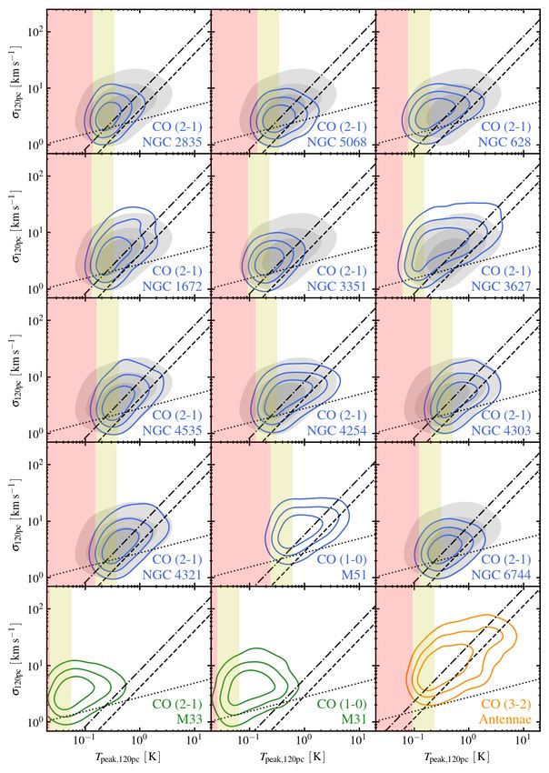
Figures 1 and 2 show the distribution of molecular gas central region of disk galaxies has different properties com-
mass (as inferred from CO flux) for each galaxy as a func- pared to the gas in the disk (e.g., Oka et al. 2001; Regan et al.
tion of molecular gas surface density, Σ, measured at 80 and 2001; Jogee et al. 2005; Shetty et al. 2012; Kruijssen & Long-
120 pc resolution respectively. Figures 3 shows the corre- more 2013; Colombo et al. 2014a; Leroy et al. 2015; Free-
sponding distributions as a function of velocity dispersion, σ, man et al. 2017, among many others). Especially in galaxies
measured at 120 pc resolution. For each galaxy, we include with strong bars, the inner parts of galaxies often harbor high
all sightlines with detected CO emission across the whole gas surface densities and complex structures such as starburst
field of view (FoV). rings (Kenney et al. 1992; Sakamoto et al. 1999; Sheth et al.
For most of the molecular gas properties considered in this 2002; Kormendy & Kennicutt 2004; Jogee et al. 2005).
work, their median values often show systematic variation To illustrate the impact of nuclear gas concentrations, we
across the spatial scales that we consider, while the shape define a central region for each galaxy. In Figures 1–3, we
of their distribution functions and the rank order of galxies plot the distribution for gas in this central region and the outer
barely varies. Therefore in the following part of this section, disk as separate histograms (dotted and dashed lines). For
most of the tables report the median values and widths of most galaxies, we define the center as the region within 1 kpc
all the relevant measurements at 45, 80, and 120 pc scales, of the galaxy nucleus. For NGC 3351, we slightly expand the
while most of the figures only illustrate results at 120 pc scale defined radius to 1.5 kpc, so that the visually distinct inner
(where we have available data for all targets). disk is entirely designated as central. The central regions of
M31 and NGC 6744 are not included in our CO data, and the
CO map of the Antennae only covers the interacting region.
5.1.1. Central and Disk Distributions Therefore we do not plot any separate histograms for these
For many of the galaxies with the widest range of Σ and σ, galaxies.
we observe multiple peaks in the Σ and σ distributions (e.g., Comparing the “center” distributions to the “disk” dis-
NGC 3351, NGC 3627, NGC 1672, NGC 4535, NGC 4303, tributions, we find that for the strongly barred galaxies
and NGC 4321). By visually inspecting the maps in Figure (NGC 3351, NGC 3627, NGC 1672, NGC 4535, NGC 4303,
A1, we see that the high value peak(s) of Σ and σ tend to and NGC 4321) the peaks of the distribution at large valuesC LOUD -S CALE M OLECULAR G AS P ROPERTIES IN 15 N EARBY G ALAXIES 11 Figure 1. Distribution of molecular gas mass as a function of surface density, Σ, measured at 80 pc resolution. Each panel shows results for one galaxy, with the target name, bar type (in the brackets), and CO flux recovery fraction fM indicated in the top right corner. We order the targets from left to right, then top to bottom, following the scheme in Table 2. Galaxies in the “main sample” (PHANGS-ALMA targets plus M51) are represented by blue color, the Local Group targets by green color, and the Antennae by orange color (this color scheme is used consistently throughout this paper). All curves show Gaussian kernel density estimators (KDE) generated from the data with bandwidth of 0.1 dex in logarithmic space. The solid curve shows the distribution for all sightlines with CO detections across the whole field of view (FoV). The dashed/dotted curves show the distribution of mass for galaxy disk/central regions (usually defined as outside/inside the rgal = 1 kpc boundary), respectively. The vertical dashed line and color shaded region show the mass weighted median value and 16-84% range of Σ for the “disk” population, while the vertical dotted line shows the median Σ for the “center”. The hatched region has less than 100% completeness due to limited sensitivity of the data. Individual galaxy disks typically have most of their molecular gas spread over a 0.5-1.0 dex range of Σ, and both the median of this distribution and its width vary from galaxy to galaxy. Our strongly barred targets show significantly different distributions for the disk and central regions, see NGC 3351, NGC 3627, and more examples in Figure 2.
12                                                              S UN ET AL .

Figure 2. As in Figure 1, but here showing the Σ distribution at 120 pc resolution for all 15 targets. The general sense of galaxy-by-galaxy
variations is more clearly revealed in this figure: higher mass star-forming galaxies tend to keep more gas at high Σ (note that the CO map
of NGC 6744 does not cover the central region, which might be the reason of this target being an outlier from the general trend). Note that
all strongly barred galaxies (NGC 1672, NGC 3351, NGC 3627, NGC 4535, NGC 4303, and NGC 4321) demonstrate significant disk/center
dichotomies in their Σ distribution.
C LOUD -S CALE M OLECULAR G AS P ROPERTIES IN 15 N EARBY G ALAXIES                                                 13

Figure 3. Distribution of molecular gas mass as a function of velocity dispersion, σ, measured at 120 pc resolution. All curves are Gaussian
KDE generated from the data with bandwidth of 0.1 dex in logarithmic space. Labels and line-styles have the same meanings as in Figure 1
and 2, except that the hatched region here shows the σ range close to or below the spectral resolution limit. Galaxies show distributions of mass
as a function of σ similar to their Σ distributions (Figure 1), but the dynamical range in σ is only about half of that seen in Figure 2.
14                                                    S UN ET AL .

                                 Table 4. Properties of the Σ Distribution Function

        Galaxy             at 45 pc resolution              at 80 pc resolution           at 120 pc resolution

                      disk        disk      center    disk         disk      center    disk       disk     center
                    median      16-84%     median    median      16-84%     median    median    16-84%     median
                    log10 Σ      width     log10 Σ   log10 Σ      width     log10 Σ   log10 Σ    width     log10 Σ

      NGC 2835        1.75        0.56       1.91     1.49         0.59       1.61     1.36      0.60       1.46
      NGC 5068        1.78        0.52       1.79     1.55         0.59       1.51     1.44      0.57       1.40
      NGC 628         1.78        0.64       1.83     1.58         0.72       1.72     1.48      0.71       1.67
      NGC 1672         –           –             –      –           –             –    1.84      0.96       3.04
      NGC 3351         –           –             –    1.42         0.53       2.95     1.26      0.54       2.89
      NGC 3627         –           –             –    2.23         1.08       3.15     2.17      1.06       2.97
      NGC 4535         –           –             –      –           –             –    1.78      0.82       2.93
      NGC 4254         –           –             –      –           –             –    2.03      0.81       2.47
      NGC 4303         –           –             –      –           –             –    1.98      0.71       2.82
      NGC 4321         –           –             –      –           –             –    1.84      0.86       2.94
      M51             2.43        0.77       2.47     2.33         0.83       2.41     2.26      0.84       2.39
      NGC 6744         –           –             –    1.64         0.59           –    1.53      0.60            –
      M31             1.24        0.65           –    1.09         0.68           –    1.03      0.65            –
      M33              –           –             –    0.99         0.76       1.21     0.89      0.73       1.16
      Antennae         –           –             –    3.41         1.16           –    3.37      1.18            –

     N OTE—For each galaxy at each resolution, we report: (1) median log10 Σ value by gas mass for the “disk”
      population (in units of M pc−2 ); (2) full width of the 16-84% gas mass range of Σ distribution for the “disk”
      population (in units of dex); and (3) median log10 Σ value by gas mass for the “center” population (in units of
      M pc−2 ).
You can also read