Reproducible determination of dissolved organic matter photosensitivity
←
→
Page content transcription
If your browser does not render page correctly, please read the page content below
Biogeosciences, 18, 3367–3390, 2021
https://doi.org/10.5194/bg-18-3367-2021
© Author(s) 2021. This work is distributed under
the Creative Commons Attribution 4.0 License.

Reproducible determination of dissolved organic
matter photosensitivity
Alec W. Armstrong1,2 , Leanne Powers1 , and Michael Gonsior1
1 Chesapeake Biological Laboratory, University of Maryland Center for Environmental Science,
Solomons, Maryland 20688, USA
2 Department of Entomology, University of Maryland, College Park, Maryland 20742, USA

Correspondence: Alec W. Armstrong (aarmstr1@umd.edu) and Michael Gonsior (gonsior@umces.edu)

Received: 3 June 2020 – Discussion started: 2 July 2020
Revised: 24 March 2021 – Accepted: 15 April 2021 – Published: 7 June 2021

Abstract. Dissolved organic matter (DOM) connects aquatic         to compare DOM photosensitivity in two adjacent freshwa-
and terrestrial ecosystems, plays an important role in carbon     ter wetlands as seasonal hydrologic changes alter their DOM
(C) and nitrogen (N) cycles, and supports aquatic food webs.      sources.
Understanding DOM chemical composition and reactivity is
key for predicting its ecological role, but characterization is
difficult as natural DOM is comprised of a large but unknown
number of distinct molecules. Photochemistry is one of the        1   Introduction
environmental processes responsible for changing the molec-
ular composition of DOM, and DOM composition also de-             The photochemical reactivity of dissolved organic matter
fines its susceptibility to photochemical alteration. Reliably    (DOM) is inherently linked to its composition, and its pho-
differentiating the photosensitivity of DOM from different        tochemical behavior reflects compositional differences be-
sources can improve our knowledge of how DOM composi-             tween samples. Several authors have discussed the funda-
tion is shaped by photochemical alteration and aid research       mental processes involved in light absorption by DOM and
into photochemistry’s role in various DOM transformation          the phenomena that may follow (Miller, 1998; Sharpless et
processes. Here we describe an approach for measuring and         al., 2014), including loss of absorbance (Del Vecchio and
comparing DOM photosensitivity consistently, based on the         Blough, 2002), production of new substances (Gonsior et al.,
kinetics of changes in DOM fluorescence during 20 h pho-          2014; Blough and Zepp, 1995; Bushaw et al., 1996; Moran
todegradation experiments. We identify several methodologi-       and Zepp, 1997), and loss of fluorescence (Blough and Del
cal choices that affect photosensitivity measurements and of-     Vecchio, 2002). Absorption spectra and derived values, such
fer guidelines for adopting our methods, including the use        as spectral slopes and their ratios, have long been used to
of reference material, precise control of conditions affect-      characterize DOM (Blough and Del Vecchio, 2002; Helms
ing photon dose, leveraging actinometry to estimate pho-          et al., 2008; Twardowski et al., 2004). Fluorescence mea-
ton dose instead of expressing results as a function of ex-       surements arise from only a fraction of chromophoric DOM
posure time, and frequent (every 20 min) fluorescence and         (CDOM) but are sensitive to small variations in DOM chem-
absorbance measurements during exposure to artificial sun-        ical composition (Blough and Del Vecchio, 2002). To the
light. We then show that our approach can generate photo-         extent that photochemical reactivity is a property of DOM
sensitivity metrics across several sources of DOM, includ-        chemical composition (Boyle et al., 2009; Cory et al., 2014;
ing freshwater wetlands, a stream, an estuary, and Sargas-        Del Vecchio and Blough, 2004; Gonsior et al., 2013, 2009;
sum sp. leachate and observed differences in these metrics        Wünsch et al., 2017), comparing the potential for photo-
that may help identify or explain differences in their compo-     chemical transformation of different DOM sources or treat-
sition. Finally, we offer an example of applying our approach     ments (hereafter called photosensitivity) may be a useful tool
                                                                  in the continuing effort to characterize DOM composition

Published by Copernicus Publications on behalf of the European Geosciences Union.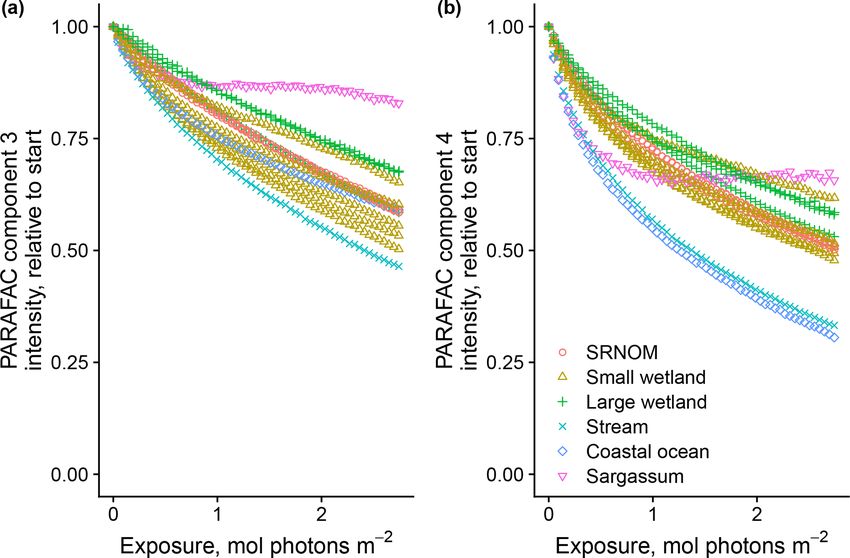
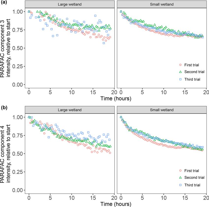
3368                    A. W. Armstrong et al.: Reproducible determination of dissolved organic matter photosensitivity

and to describe its susceptibility to sunlight-induced degrada-   active components. Fluorescence losses were best described
tion. Such comparisons require robust methods that are sen-       by the sum of two exponential decay terms, allowing straight-
sitive enough to discern ecologically and chemically relevant     forward and precise modeling of photosensitive fluorescence
differences between distinct DOM sources.                         signals that degraded quickly, which may reflect chemically
   Research across ecosystem settings has measured changes        distinct processes contributing to fluorescence loss during
in optical properties following sunlight or simulated-sunlight    photodegradation. This approach may offer the resolution
irradiation to infer changes in DOM composition. A gen-           required to compare photosensitivity between samples with
eral discussion of this approach and its bases has been previ-    small, but ecologically significant, differences in DOM com-
ously published (Hansen et al., 2016; Kujawinski et al., 2004;    position.
Sulzberger and Durisch-Kaiser, 2009). Examples of recent             The goals of this study are to (1) identify methodologi-
research, using photochemical changes to make ecologically        cal barriers to reproducible determination of DOM photo-
significant distinctions between DOM samples collected in         sensitivity and offer experimental guidelines to improve the
specific ecosystems, have been described in detail elsewhere      studies of DOM photodegradation kinetics, (2) test our ap-
(Gonsior et al., 2013; Laurion and Mladenov, 2013; McEn-          proach on samples from various environmental settings to
roe et al., 2013; Minor et al., 2007). DOM photodegrada-          see if our derived metrics of photosensitivity might respond
tion itself has ecological consequences, affecting overall car-   to variability in DOM composition, and (3) analyze photo-
bon (C) cycling (Anesio and Granéli, 2003; Obernosterer and       sensitivity differences between different DOM sources in de-
Benner, 2004), microbial heterotrophy of DOM (Amado et            tail to better understand the links between DOM composi-
al., 2015; Cory et al., 2014; Lapierre and del Giorgio, 2014),    tion, environmental setting, and photochemical degradation
and algal and submerged plant primary productivity (Arrigo        processes. In a series of experiments, we explored poten-
and Brown, 1996; Thrane et al., 2014).                            tial sources of variability in photodegradation kinetics stem-
   Experimental approaches connecting DOM chemical                ming from experimental conditions and methodology. We
composition, its optical properties and their photochemical       further develop a previously described experimental setup
bases, and relevant ecological phenomena typically expose         (Timko et al., 2015), showing that results are reproducible
natural DOM samples to natural or simulated sunlight and          under controlled conditions using a common reference mate-
measure the change in optical properties over time. In situ ex-   rial, and suggest a set of best practices for collecting repro-
periments have been used to explore the role of photodegra-       ducible and high-resolution time series of fluorescence mea-
dation relative to other transformations of DOM in aquatic        surements during experimental irradiation of a single sample.
ecosystems, but field studies are difficult, if not impossible,   Then we apply this approach to several natural DOM sources
to reproduce (Cory et al., 2014; Groeneveld et al., 2016; Lau-    by building on and exploring new dimensions of an estab-
rion and Mladenov, 2013). Laboratory-based irradiation ex-        lished modeling framework (Murphy et al., 2018) to iden-
periments may allow greater reproducibility and logistical        tify photosensitivity differences that may be ecologically rel-
flexibility. Laboratory photodegradation experiments have         evant. Finally, we thoroughly test DOM from two wetlands to
tested the potential ecological significance of photodegra-       show how these differences in photosensitivity metrics may
dation and explored the fundamental photochemical mecha-          help us link DOM composition to ecological phenomena.
nisms involved in photobleaching (Chen and Jaffé, 2016; Del
Vecchio and Blough, 2002; Goldstone et al., 2004; Hefner et
al., 2006). These experiments usually involve the simultane-      2     Materials and procedures
ous irradiation of DOM in several sample vials under poly-
chromatic or monochromatic light. Vials are then destruc-         2.1    Photoirradiation system
tively sampled for DOM measurements at intervals through-
out the experiment or simply compared before and after light      We needed our system to irradiate samples without self-
exposure. While powerful, these experiments require a trade-      shading, even at relatively high CDOM concentrations. The
off in effort between the reproducibility and temporal reso-      photoirradiation system circulates an aqueous sample be-
lution. Replicate vials are often sampled to ensure precision     tween a mixing reservoir (i.e., equilibration flask), a solar
and improve reproducibility, but lamp space is finite, limiting   simulator, and a spectrofluorometer, similar to a system de-
the temporal sampling resolution.                                 scribed previously (Timko et al., 2015). A photograph of
   Continuous measurement of a single sample undergoing           the system can be found in Appendix A (Fig. A1). Sam-
controlled photoirradiation offers an alternative experimen-      ples were continuously circulated between a central mixing
tal approach. The kinetics of DOM fluorescence loss during        reservoir, and system components were connected by PEEK
photoirradiation experiments have been recently described         tubing (LEAP PAL Parts + Consumables, LLC; 0.062500
(Murphy et al., 2018; Timko et al., 2015). These studies          (1.587 mm) outside diameter; 0.03000 (0.762 mm) inside di-
leveraged novel time series of frequent measurements (e.g.,       ameter). The central reservoir was a 25 mL borosilicate equi-
every 20 min) of fluorescence and ultraviolet–visible (UV–        librator flask with a magnetic stir bar constantly rotating at
Vis) absorption, which allowed the modeling of distinct re-       its bottom at a speed low enough to prevent visible bub-

Biogeosciences, 18, 3367–3390, 2021                                                 https://doi.org/10.5194/bg-18-3367-2021
A. W. Armstrong et al.: Reproducible determination of dissolved organic matter photosensitivity                            3369

bles from forming. Sample gently dripping from flow lines          lar irradiance was modeled, using the system for transfer of
into the equilibrator ensured that sample remained oxy-            atmospheric radiation model (Ruggaber et al., 1994), and cal-
genated during photodegradation. A micro-gear pump (HNP-           culated just below the water surface as described previously
Mikrosysteme; mzr-4665) was used to pump the sample with           (Fichot and Miller, 2010). With 10 mL volume added to the
an almost pulseless flow through the system at a rate of           equilibrator (our typical experimental conditions), a 20 h ir-
1.5 + 0.1 mL min−1 . The spectrophotometer flow cell and           radiation experiment was equivalent to 1.0 d of exposure be-
equilibrator flask were surrounded by a circulating water          tween 330–380 nm at 45◦ N latitude in mid-July where 1 d
jacket set to 25 ◦ C. To prevent contamination or the estab-       is ∼ 15.75 h long. For the lowest total volume used here
lishment of microbes that could degrade DOM during experi-         (0.5 mL in the equilibrator; total volume 12.7 mL), photon
ments, the system was flushed with 0.1 M NaOH between ex-          dose was 1.7 times higher than this estimate. We calculated
periments and then thoroughly flushed with ultrapure water.        a mean photon flux of 3.9 × 10⁻⁵ mol photons m−2 s−1 for
Ultrapure water for blanks was circulated for at least 10 min      experiments, with 10 mL sample added once flow lines were
before checking the absorbance and fluorescence for signs of       filled (total sample volume 22.2 mL), based on a mean pho-
contamination. If blank contamination persisted after subse-       ton exposure of 0.23 µmol photons cm−2 min−1 (five trials;
quent rinses, the system was flushed with isopropanol and          standard deviation 0.0045).
thoroughly rinsed with ultrapure water before checking for             Past experiments revealed the importance of pH control on
contamination by examining optics and testing (DOC).               DOM fluorescence and photodegradation kinetics (Timko et
   Samples were irradiated as they were slowly pumped              al., 2015). We adjusted the initial sample pH to 3.0 (+0.2)
through a custom-built flow cell (SCHOTT AG BO-                    with HCl but did not control pH by autotitration. At pH 3.0,
ROFLOAT borosilicate glass; Hellma Analytics; 70 % to              natural organic acids should generally be protonated, regard-
85 % transmission between 300 and 350 nm; 85 % transmis-           less of compositional differences between DOM sources,
sion at wavelengths > 350 nm), with a total exposure path          which should prevent solution pH change due to the pho-
area of 101 cm2 arranged in an Archimedean spiral and re-          toproduction of CO2 (Ritchie and Perdue, 2003). Starting at
turned to the equilibrator flask. This 20 × 20 cm borosilicate     pH 3.0, and equilibrating the sample in an air-filled reaction
spiral flow cell had a 1 mm deep × 2 mm wide long flow path        vessel, ensured minimal pH change during irradiation, and
covering the irradiation area and was located underneath a         it never changed by more than 0.2 pH units, which is in line
solar simulator (Oriel Sol2A) with a 1000 W Xenon arc lamp         with expectations from work on mechanisms explaining pH
equipped with an air mass (AM) 1.5 filter. Lamp output was         decreases during photooxidation (Xie et al., 2004).
checked periodically, using an Oriel PV reference cell set to
one sun, which corresponds here to exactly 1000 W m−2 , and        2.2   Optical measurements
lamp power was held constant during irradiation experiments
using a Newport 68951 digital exposure controller. Another         We used a HORIBA Jobin Yvon Aqualog spectrofluorome-
tubing carried the sample from the equilibrator flask to a         ter to collect the time series of UV–Vis absorbance and exci-
temperature-controlled square quartz fluorescence flow cell        tation emission matrix (EEM) fluorescence spectra through-
(1 cm × 1 cm) located within a HORIBA Jobin Yvon Aqua-             out the experiments. UV–Vis absorbance was measured at
log spectrofluorometer.                                            3 nm intervals between 600 and 230 nm. Fluorescence ex-
   Total sample exposure varied, depending on the total vol-       citation occurred at the same intervals, and emission spec-
ume in the photodegradation system. We controlled volume           tra were recorded from 600 to 230 nm at 8 pixel charged
by completely filling the tubing and flow cells (12.2 mL vol-      coupled device (CCD) resolution or, approximately, 3.24 nm
ume) and adjusting the volume added to the equilibration           intervals. EEMs integration times were 1 s. Milli-Q water
flask. We used nitrite actinometry to calculate photon flux,       (18.2 M cm), adjusted to pH 3.0 with concentrated HCl,
based on the response bandwidth between 330 and 380 nm of          was circulated through the system and used as a measure-
the nitrite actinometer (Jankowski et al., 1999, 2000). Briefly,   ment blank immediately prior to each experiment.
a solution of 1 mM sodium nitrite, 1 mM benzoic acid, and
2.5 mM sodium bicarbonate was circulated through the irra-         2.3   Experiments
diation system, with regular measurements of fluorescence
emission at 410 nm after excitation at 305 nm. Results are         Several sets of experiments explored method reproducibil-
compared against a fluorescence calibration curve using 0–         ity, sensitivities to experimental conditions, and differences
5 µm salicylic acid fluorescence to calculate the formation of     between DOM sources. For our first goal of identifying
salicylic acid from benzoic acid (mediated by hydroxyl rad-        methodological barriers to the reproducible determination of
icals formed during the photolysis of nitrite) as a function       DOM photosensitivity, we varied the concentrations and vol-
of time. This is then used to calculate photon exposure as         umes of Suwannee River natural organic matter (SRNOM)
a function of time. Actinometer experiments were repeated          PPL (Priority PolLutant) extracts added to the photodegra-
with 0.5, 5, and 10 mL of actinometer solution added to the        dation system to test their influence on degradation kinetics.
equilibration vessel after filling flow lines. Average July so-    Different researchers in our group then repeated the experi-

https://doi.org/10.5194/bg-18-3367-2021                                                  Biogeosciences, 18, 3367–3390, 2021
3370                   A. W. Armstrong et al.: Reproducible determination of dissolved organic matter photosensitivity

ments with SRNOM PPL extracts to test reproducibility. We        collection through combusted (500 ◦ C) Whatman GF/F fil-
explored the effects of storage time on filtered water sam-      ters and acidified to pH 2.0, using concentrated HCl (Sigma-
ple photodegradation results. We then compared SRNOM             Aldrich; 32 % pure) before solid-phase extraction. The true
PPL extracts and SRNOM reference material isolated by re-        pore size used in this prefilter step was probably smaller than
verse osmosis reconstituted in ultrapure water (RO SRNOM)        0.7 µm (e.g., 0.3 µm in Nayar and Chou, 2003). All samples,
to test the effect of extraction on photodegradation kinetics.   whether whole water or solid-phase extracts redissolved in
We approached our second goal – demonstrating the util-          water, were filtered through syringe-mounted 0.2 µm cellu-
ity of our approach as a measure of DOM photosensitivity         lose acetate filters that were prerinsed with > 30 mL ultra-
– by applying methodological guidelines developed in our         pure C-free water.
tests of SRNOM to PPL extracts of DOM from a variety of             Samples from the two freshwater wetland sites are used
aquatic ecosystem settings and sources (see Sect. 2.4). Fi-      in the more detailed comparison presented in Sect. 3.3, and
nally, we ran experiments comparing the photosensitivity of      hence, these sites merit additional description. Small topo-
DOM sampled from two adjacent freshwater sites in different      graphic depressions are common throughout the interior of
seasons to better understand the links between DOM compo-        Delmarva Peninsula. These depressions persist in this low-
sition, environmental setting, and photochemical degradation     elevation, low-relief landscape, and regular seasonal inunda-
processes.                                                       tion has led to the development of wetland soils and biota in
   In each experiment, a sample was exposed to 20 h of sim-      many of these depressions. Depressions on land not drained
ulated sunlight, and EEM spectra were collected (using the       for agriculture are inundated for several months during most
“Sample Q” feature in Aqualog software), starting immedi-        years. Some do not exchange water through surface flow
ately before irradiation began, with a 17.5 min interval be-     with perennial stream networks, while others sustain down-
tween each scan, generating a time series of 60 EEM spectra      stream connections through temporary surface channels for
for each experiment. Where applicable, the time of EEM col-      several months in the wettest months of the year (typically
lection was converted to cumulative photon exposure (moles       late winter–spring). These two sites, referred to as the smaller
of photons per square meter) by multiplying time by calcu-       wetland and larger wetland, respectively, are adjacent but lie
lated photon flux (moles of photons per square meter per         within distinct topographic depressions. Their inundated ar-
second), using actinometry results generated with the same       eas expand and contract with water level fluctuations, and
sample volume.                                                   both may go entirely dry at the surface in the summer. If wa-
                                                                 ter levels are sufficiently high, their surface waters merge,
2.4    Sample materials                                          and a temporary channel may fill and sustain export flow to
                                                                 the perennial stream network. Of the sampling sites, one is
We used Suwannee River natural organic matter (SRNOM)            within the smaller depression, which mostly lacks submerged
obtained from the International Humic Substances Society         and emergent vegetation and is hemmed closely by trees. The
(IHSS) as a reference material (catalog no. 2R101N; iso-         other site is within a larger depression, where surface water
lated by reverse osmosis; Green et al., 2014). Freeze-dried      is more exposed to light and features a variety of herbaceous
SRNOM was dissolved in Milli-Q water and was prepared            submerged and aquatic plants. Experiments were run with
less than 1 week prior to use (hereafter called RO SRNOM).       DOM from both sites, sampled on three dates (5 October,
Dilutions approximately corresponded to a dissolved organic      20 December 2017, and 1 April 2018).
carbon (DOC) concentration of 5 mg C L−1 . This is well be-         Except for RO SRNOM samples used to test the effect of
low the DOC range found in SRNOM source material be-             solid-phase extraction and wetland samples used for the stor-
fore it was extracted but within the range of other aquatic      age time experiment described below, all samples were solid-
DOM sources dominated by terrestrially derived DOM. Ad-          phase extracted, using a proprietary styrene divinyl benzene
ditionally, SRNOM solid phase extracts, using the Agilent        polymer resin (Agilent PPL Bond Elut), following a proce-
PPL (Priority PolLutant) resin, were extracted in May 2012       dure described previously (Dittmar et al., 2008). PPL ex-
during the same time that the SRNOM standard material was        tracts were used because our goal is to develop a reproducible
isolated and were prepared directly before irradiation exper-    method to compare the photochemical behavior of natural
iments (see details below).                                      organic matter without the influence of the sample matrix.
   Additional water samples were collected across a vari-        Extracts allow longer storage, isolate organic matter from
ety of aquatic ecosystems to explore the range of our ap-        potentially photosensitive matrices, and capture representa-
proach and to validate it. Sample sources include two fresh-     tive photosensitive organic matter fractions (Murphy et al.,
water wetland sites (Caroline County, Maryland, USA), one        2018). While filtration to 0.2 µm should remove most viable
perennial stream (Parkers Creek, Calvert County, Maryland,       microbes, microbial degradation may still be possible in fil-
USA; collected September 2017), one estuary (Delaware            tered water if ultra-small microorganisms are present (Brails-
Bay, USA; collected July 2016), and leachate from live Sar-      ford et al., 2017; Luef et al., 2015). Extraction removes this
gassum sp. collected in Bermuda in July 2016 (Powers et          possibility.
al., 2019). These samples were 0.7 µM filtered within 24 h of

Biogeosciences, 18, 3367–3390, 2021                                                 https://doi.org/10.5194/bg-18-3367-2021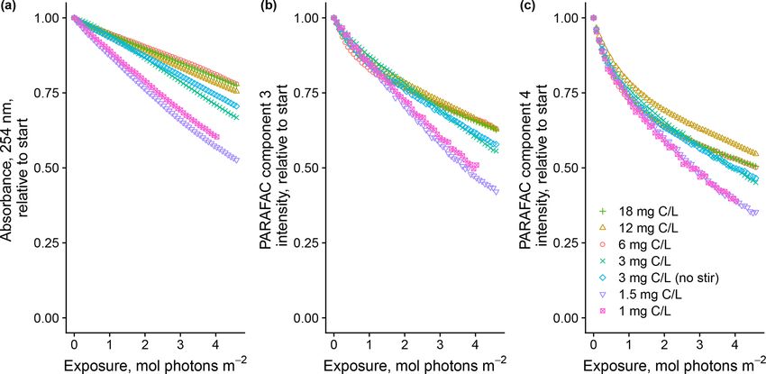
A. W. Armstrong et al.: Reproducible determination of dissolved organic matter photosensitivity                            3371

   Immediately prior to each experiment, 0.5–5 mL of the ex-      below 270 nm were excluded, due to high leverage on models
tract was evaporated under high-purity N2 gas, dissolved in       that led to noisy loading spectra and for ready comparison to
30 mL ultrapure C-free Milli-Q water, and diluted to simi-        the PARAFAC models presented elsewhere (Murphy et al.,
lar CDOM absorbance values to minimize any potential in-          2018). The full data set of EEMs from all degradation exper-
ner filter effects on fluorescence degradation kinetics. Ab-      iments was then projected onto the four-component model
sorbance (A) at 300 nm was used as a benchmark for dilution       derived from SRNOM PPL. This allowed the standardization
instead of adjustments based on measured DOC because it           of the fluorescence signal loss we wished to model. Fluores-
could be done quickly on the equipment used for the photo-        cence intensity at the maximum of each component (Fmax)
chemical experiments and allowed the consistent correction        was normalized to the second data point in each degradation
of inner filtering effects. We adjusted all samples (except for   experiment time series, as the first points (collected immedi-
those used in the storage time experiments described below)       ately before lamp exposure) were often outliers with aberrant
to a raw absorbance of 0.12 (+0.01), which translates to a        residuals after modeling fluorescence losses (e.g., Eqs. 2 and
Napierian absorption coefficient (a) of 27.6 m−1 . Delaware       3).
Bay samples were too diluted to generate sufficient volume           Previous studies (Murphy et al., 2018; Del Vecchio and
to fill the photoirradiation system, so several sample extracts   Blough, 2002) used a biexponential model to describe fluo-
from throughout the depth profile of a single sample station      rescence loss during photo-exposure, as described in Eq. (2),
were combined prior to evaporation.                               as follows:

2.5   Data analyses                                               ft = fL e−kL t + fSL e−kSL t ,                             (2)
                                                                  where ft , total fluorescence normalized to the first EEM col-
Fluorescence EEM spectra were inner filter corrected and          lected after the solar simulator lamp shutter opened at time
had first-order Rayleigh scatter removed by the built-in          t, is the sum of two fluorescence fractions (fL and fSL ) un-
Aqualog software (based on origin). Second-order Rayleigh         dergoing decay at different rates (kL and kSL ; Murphy et al.,
scatter was removed using an in-house MATLAB toolbox,             2018; Timko et al., 2015).
following methods previously described (Zepp et al., 2004).          We modified Eq. (2) to replace time t with cumulative
EEM spectra were normalized by dividing fluorescence mea-         photon dose, assuming the lamp photon output is constant
surements by the area of the Raman scatter peak of the wa-        throughout each experiment. If it can be properly measured,
ter blanks. Data were processed in MATLAB R2018a, using           using cumulative photon exposure instead of time as the in-
an in-house toolbox and the drEEM toolbox (Murphy et al.,         dependent variable in models of fluorescence loss may al-
2013). Absorbance data were converted to absorption coeffi-       low better comparison of parameters between experiments,
cients using Eq. (1) as follows:                                  researchers, and experimental setups. The model is given in
a (λ) = 2.303A(λ)/ l,                                      (1)    Eq. (3) as follows:
                                                                  fP = fL e−kL P + fSL e−kSL P ,                             (3)
where a is the absorption coefficient at wavelength λ, A is
raw absorbance at wavelength λ, and l is path length in me-       where fP is total normalized fluorescence after cumulative
ters (here 0.01; Hu et al., 2002).                                photon exposure P (in moles of photons per square meter).
    We fitted a four-component parallel factor analysis           Other variables are the same as in Eq. (2). Photon dose es-
(PARAFAC) model to data from three SRNOM PPL extract              timations from nitrite actinometry can be applied to DOM
experiments (60 EEMs each; 180 EEMs in total). PARAFAC            irradiated under the same conditions if those conditions al-
models with three, four, and five components were fitted to       low for optically thin solutions during exposure. The 1 mm
the three SRNOM PPL extract experiment EEMs. The four-            path length spiral exposure cell we used should ensure opti-
component model was chosen as it exhibited better compo-          cal thinness, even in highly absorbent DOM solutions.
nent spectral characteristics than the others. Emission spectra      Results from fitting Eq. (3) are reported as four separate
from the components matched the four components identi-           parameters, i.e., fL , kL , fSL , and kSL . However, fL and fSL
fied in similar experiments (Murphy et al., 2018). Split-half     are not independent as they should always sum to 1. They are
validation is often used to validate PARAFAC models fitted        expressed separately in our results because we believe these
to data sets where each EEM represents a different DOM            f values may be useful for understanding the compositional
source but may not be appropriate for data sets where EEMs        bases of degradation differences, despite the difficulties for
are not independent. Instead, four-component models were          interpretation this dependence presents, and because each f
fitted from each of the three SRNOM PPL extract exper-            value was fitted separately, so modeled fits do not always sum
iments individually to confirm that each experiment’s data        exactly to 1.
led to the same PARAFAC model, and then the model built              R software (v. 3.6.0) was used to fit biexponential models
from all three experiments was compared to each of these.         using the nlsLM function from the minpack.lm package, and
All comparisons were confirmed using Tucker congruence            R was also used for significance testing and plotting most
(rex ×rem >0.99 for all components in all cases. Wavelengths      results.

https://doi.org/10.5194/bg-18-3367-2021                                                    Biogeosciences, 18, 3367–3390, 2021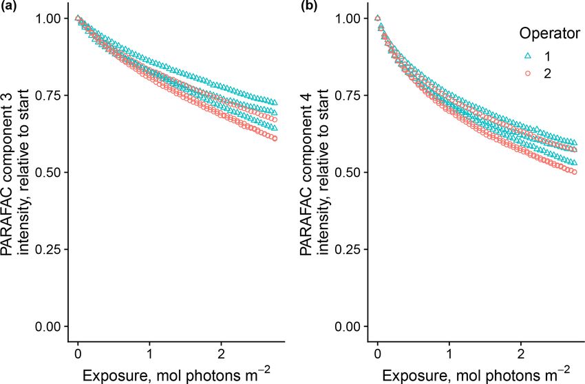
3372                    A. W. Armstrong et al.: Reproducible determination of dissolved organic matter photosensitivity

3     Results and discussion                                      pattern, while component two showed little net change. Dif-
                                                                  ferences in PARAFAC component matches and behavior be-
We stated three goals of this study, claiming we would            tween this study and Murphy et al. (2018) could arise from
(1) identify methodological barriers to the reproducible de-      operating at a different pH (3.0 here vs. their minimum pH
termination of DOM photosensitivity and offer experimental        of 4.0). For example, despite spectral differences, component
guidelines to improve studies of DOM photodegradation ki-         one behaves similarly to F420 in Murphy et al. (2018), which
netics, (2) test our approach on samples from various envi-       showed less rapid initial decay and a more linear overall pat-
ronmental settings to see if our derived metrics of photosen-     tern as pH decreased from 8 to 4 (see Fig. S4 in Murphy et
sitivity might respond to variability in DOM composition,         al., 2018). Further results will focus on components three and
and (3) analyze photosensitivity differences between differ-      four as they are most sensitive to photodegradation.
ent DOM sources in detail to better understand the links be-
tween DOM composition, environmental setting, and pho-            3.1.2   SRNOM experiments – experimental conditions
tochemical degradation processes. Our results are presented               and photon dose
and discussed in the same order. Section 3.1 discusses ex-
periments using SRNOM that identify several sources of ex-        Photodegradation kinetics in SRNOM trials were sensitive to
perimental variability that influence photodegradation results    many experimental conditions but most importantly to those
which are crucial for applying our approach with confidence       that affected cumulative photon exposure. Key influences in-
but also relevant to other methods of experimental DOM pho-       cluded the volume of the sample added to the irradiation sys-
todegradation. Section 3.2 shows that we were able to suc-        tem and DOM concentration, and we also tested for differ-
cessfully apply our method to experiments using several dif-      ences in results due to unknown discrepancies between in-
ferent DOM sources. Finally, Sect. 3.3 presents a detailed        dividual researchers. Measurements made as a function of
comparison of experiments using samples from two freshwa-         exposure time could obscure these differences if photon ex-
ter wetlands to discuss the ecological relevance of photosen-     posure was not instead directly estimated. In this subsection,
sitivity differences measured with our approach. Sections 3.1     we describe these methodological influences on the results
and 3.3 are further divided into topically distinct subsections   and demonstrate the utility of directly expressing results as
for convenience.                                                  a function of estimated photon exposure instead of exposure
                                                                  time.
3.1     Method optimization and reproducibility                      Total volume of sample in the system affected degrada-
                                                                  tion kinetics by altering the cumulative photon exposure rel-
3.1.1    PARAFAC model                                            ative to the abundance of optically active molecules. Fig-
                                                                  ure 3 shows the loss of absorbance at 254 nm and loss of
Our results confirm many of the findings reported by Murphy       fluorescence intensity of components three and four, relative
et al. (2018) in that the fitted PARAFAC model of SRNOM           to starting values, in experiments where the total volume of
PPL photodegradations produced similar components de-             the sample varied. Sample volume predictably affects photon
spite the independent data collection and analysis by differ-     dose relative to the quantity of the starting material because,
ent researchers (Fig. 1). Emission maxima for components          in all trials, a fixed volume of the total volume is exposed
one to four were 439, 412, 525, and 452 nm; however, only         to light at any time before returning to the mixing vessel.
components three and four followed the biexponential de-          We found that flow rates from 1.5 to 8 mL per minute did
cay pattern. Figure 2 shows an example of the fluorescence        not impact the photon dose (data not shown). Removing the
change in each PARAFAC component during photodegrada-             magnetic stir bar in the equilibration vessel seemed to have
tion of SRNOM PPL. Component three in this study corre-           a slight effect on absorbance and, to a lesser degree, fluo-
sponds to F520 in Murphy et al. (2018), while component           rescence loss, so it was used throughout subsequent exper-
four corresponds to the F450 . Matching component spec-           iments. Expressing loss of absorbance and fluorescence as
tra to models in the online OpenFluor database confirmed          a function of estimated photon exposure rather than a func-
these matches, with Tucker congruence r values over 0.98          tion of time seems necessary to ensure comparability with
for emission spectra for both components. The weaker match        other experimental systems, and we will follow this conven-
between component four in this study and F450 in Murphy et        tion where possible.
al. (2018) is driven by differences in the excitation spectra        However, the reader is reminded that actinometers do
(r = 0.949), but strong correlations between all four compo-      have limitations (e.g., broadband response measurement)
nents in our PARAFAC model and higher information den-            and caveats exist for their successful interpretation. Because
sity in low wavelength ranges of excitation spectra could         CDOM absorption spectra generally increase exponentially
interfere with the excitation spectral signal discrimination.     with decreasing wavelengths, many experimental designs
Components one and two in this study did not exhibit biexpo-      may violate the requirement that samples are optically thin
nential decay during photodegradation. In most experiments,       when irradiated (Hu et al., 2002). The irradiation cell used
component one decayed but did not follow a biexponential          here has a depth of 1 mm, which should prevent self-shading

Biogeosciences, 18, 3367–3390, 2021                                                 https://doi.org/10.5194/bg-18-3367-2021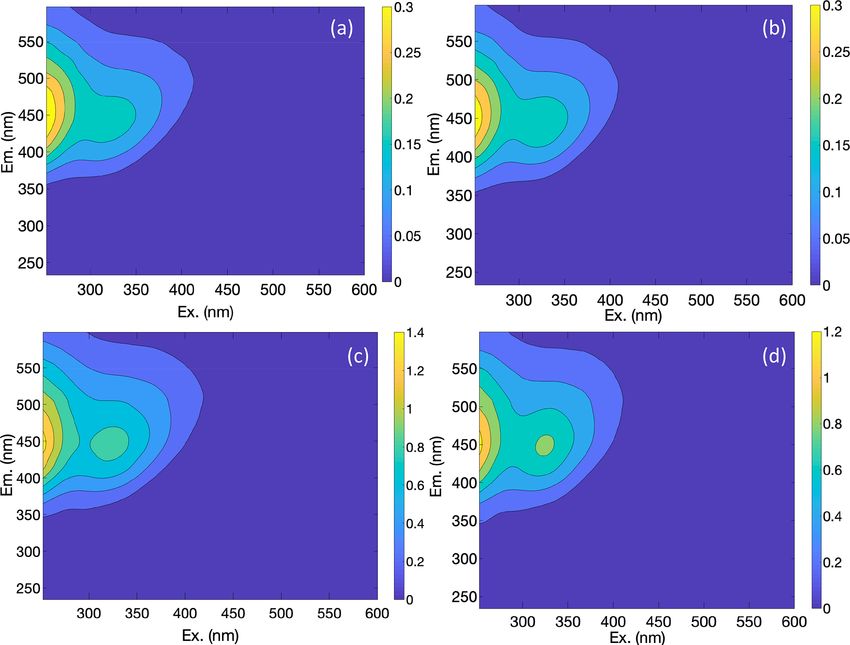
A. W. Armstrong et al.: Reproducible determination of dissolved organic matter photosensitivity                                     3373

Figure 1. (a) Spectral loadings and (b) contour plots of PARAFAC components (one–four; left to right) modeled from EEMs of SRNOM
PPL extract photodegradation time series. In the top row, the dashed lines represent excitation spectra, and the solid lines show emission
spectra. The full data set of all degradation time series EEMs was projected onto this model.

                                                                       All solutions shown here were considered optically thin at
                                                                       300 nm and greater wavelengths following the convention
                                                                       that, for optically thin solutions, the following applies:

                                                                       AT × L  1,                                                    (4)

                                                                       where AT is total (Napierian) absorption coefficient, and L is
                                                                       path length in meters (Hu et al., 2002). Although inner-filter
                                                                       corrections can be applied to correct for self-shading in spec-
                                                                       trophotometer cells with known geometry (Hu et al., 2002),
                                                                       these corrections cannot be easily applied in other irradia-
                                                                       tion designs (e.g., vials on their sides and spiral flow cells).
                                                                       The definition for optically thin solutions (Eq. 4) is some-
                                                                       what vague, so we also tested the dependence of the DOM
                                                                       concentration on photodegradation rates.
                                                                          Degradation patterns seemed to be sensitive to DOM con-
Figure 2. Example of fluorescence change in PARAFAC com-               centration as well, but the effects were less clear (Fig. 4). In
ponents during photodegradation. Data show the degradation of          general, lower concentrations showed greater overall losses
SRNOM PPL.                                                             of absorbance and fluorescence. For the two most dilute so-
                                                                       lutions, PARAFAC C3 loss could not be modeled with a bi-
                                                                       exponential model, which is in contrast to all the other sam-
during photo-exposure at all concentrations tested. Previ-             ples throughout our study. Our results suggest either that our
ous work using this system showed that fluorescence loss               solutions experienced self-shading despite meeting the con-
was independent of SRNOM concentrations between 25 and                 ventional definition of optical thinness or some other mech-
100 mg L−1 (Timko et al., 2015). Concentration dependence              anism links CDOM concentration to absorbance or fluores-
in photochemistry is often assumed to stem from self-shading           cence degradation kinetics, such as concentration-dependent
alone, and past work has shown the importance of work-                 charge transfer interactions (Sharpless and Blough, 2014).
ing with optically thin solutions or properly correcting for           Further work is needed to explain these findings.
inner-filter effects when measuring photochemical behavior.

https://doi.org/10.5194/bg-18-3367-2021                                                         Biogeosciences, 18, 3367–3390, 2021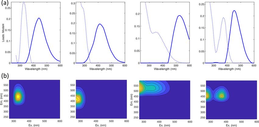
3374 A. W. Armstrong et al.: Reproducible determination of dissolved organic matter photosensitivity
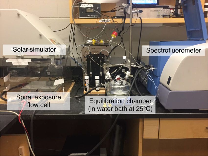
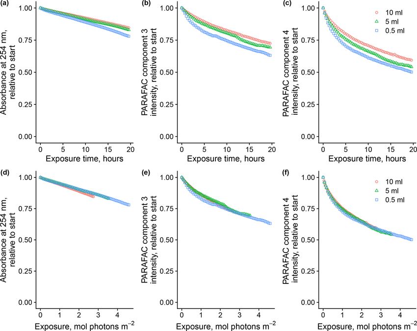
Figure 3. Photodegradation time series of absorbance at 254 nm and fluorescence intensities of PARAFAC components three and four relative
to starting values. Data are shown from experiments with SRNOM PPL that varied the volume of the sample added to the mixing reactor
(after filling flow cell lines). Panels (a)–(c) show the values as a function of exposure time, while panels (d)–(f) show the values as a function
of cumulative photon exposure calculated from NO2 / NO3 actinometry.
Of the researchers, two followed the same protocols with data did not affect these results. Fitted model parameters
the same material (SRNOM PPL) as a test of reproducibility from Eq. (3) suggest these differences stem from the kinetics
due to sample handling. Agreement between researchers was of the semilabile fluorescence pool, with possible differences
good, and results varied to a similar degree as the tests were in the relative starting abundances of the labile vs. semilabile
repeated by the same researcher (Fig. 5). The two-tailed t pools (Fig. 7; Table A1). Rate constants of the labile pool
tests were not able to distinguish differences in means be- did not vary for either PARAFAC component, suggesting ex-
tween trials run by each researcher for any biexponential traction did not affect the behavior of this pool, so studies
model parameters (p values all greater than 0.10). focusing on this pool should not be affected by PPL extrac-
tion. Capturing changes in this pool is one of the explicit ad-
3.1.3 Effects of solid-phase extraction vantages of our experimental system, and future work on en-
vironmental photoreactivity may focus on this timescale, as
Use of extracts vs. whole water samples is another major photochemical reactions in the environment are often driven
methodological choice that can affect results. Fluorescence by initial rates (Powers and Miller, 2015). However, slower
degradation from reconstituted RO SRNOM and SRNOM degradation processes or longer irradiations may be affected
PPL extracts generated the same PARAFAC components. by extraction.
However, the overall loss of modeled components three Shared PARAFAC components suggest PPL extraction did
and four differed between SRNOM PPL extracts and RO not strongly alter the compositional bases of fluorescence
SRNOM, as did kinetics of fluorescence loss (Fig. 6). The photosensitivity in the RO SRNOM, but the differences in
differences in fluorescence loss were small but systematic. losses suggest researchers should take care when comparing
The two-tailed t tests of relative fluorescence loss suggested extracts to original samples in future photodegradation ki-
differences between PPL and RO SRNOM in PARAFAC netics studies. We are not sure what gave rise to these differ-
component four (p value < 0.01), with limited support for ences, but the RO SRNOM likely contains more highly po-
differences in component three (p value = 0.06) and no sup- lar compounds, such as (poly)saccharides and related com-
port for differences in absorbance loss (p value = 0.3 for pounds (e.g., glycosates). Differences between PPL and RO
254 nm). Projecting the data onto a PARAFAC model built samples here are probably not due to variations in the pho-
from RO SRNOM degradation data instead of SRNOM PPL
Biogeosciences, 18, 3367–3390, 2021 https://doi.org/10.5194/bg-18-3367-2021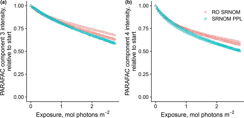
A. W. Armstrong et al.: Reproducible determination of dissolved organic matter photosensitivity                                           3375

Figure 4. Photodegradation time series of (a) absorbance at 254 nm and (b, c) fluorescence intensities of PARAFAC components three and
four, relative to the starting values. Data are shown from experiments with SRNOM PPL that varied the approximate DOC concentrations.
In all experiments, 0.5 mL SRNOM PPL solution was added to the mixing reactor after filling flow lines.

Figure 5. Photodegradation time series of PARAFAC compo-                   Figure 7. Fitted biexponential model parameters (Eq. 3) from the
nents three (a) and four (b) fluorescence intensity, relative to start-    time series of the loss of PARAFAC components three and four in
ing values. Data are shown from experiments using SRNOM PPL                irradiation experiments that compare RO SRNOM to PPL SRNOM
performed by two of the authors to test reproducibility of results.        (see Fig. 6 for data). f is unitless, and k is square meters per mole
                                                                           of photons. C3 and C4 denote PARAFAC components three and
                                                                           four. Error bars represent the mean and standard deviation from the
                                                                           three experiments. The two-tailed t tests suggest differences in kSL
                                                                           for both components (p = 0.020 in component three; p = 0.015
                                                                           in component four), while fL and fSL may differ (p = 0.065 and
                                                                           0.058) in component three. (a) kL , (b) kSL , (c) fL , and (d) fSL .

                                                                           ton dose, as volume and initial absorbance were equal across
                                                                           samples. If the concentration of fluorophores affects degra-
                                                                           dation kinetics, differing fluorophore concentrations between
Figure 6. Photodegradation time series of PARAFAC components               our PPL extracts and whole SRNOM could explain the dis-
three (a) and four (b) fluorescence intensity, relative to starting val-   crepancy. Even though we adjusted all samples to a similar
ues. Data are shown from three replicates of both RO SRNOM and             starting absorbance, selective enrichment or dilution of ab-
SRNOM PPL.                                                                 sorbing or fluorescing compounds in extracts could affect the
                                                                           mechanism responsible for any concentration dependence.
                                                                           Differences in electronic coupling and charge transfer abil-

https://doi.org/10.5194/bg-18-3367-2021                                                             Biogeosciences, 18, 3367–3390, 2021
3376                    A. W. Armstrong et al.: Reproducible determination of dissolved organic matter photosensitivity

ities (Del Vecchio and Blough, 2004; Sharpless and Blough,        sure that their procedures are generating reproducible results
2014) could arise in extracts and affect fluorescence degra-      by running several replicated experiments with reference ma-
dation kinetics. RO SRNOM may present matrix effects rel-         terial. We encourage repeating this process with multiple in-
ative to extracted SRNOM PPL, as metals and other possible        dividuals within a lab to understand the impact of individ-
interferences are still present (albeit at much lower concen-     ual methodological choices on results (e.g., gravimetric mea-
trations relative to DOC than in source water), despite the       surement of volume added vs. pipetting; preparation of sam-
cation exchange and desalting treatments that accompanied         ples). We strongly encourage at least reporting actinometry
the original reverse osmosis isolation (Kuhn et al., 2014).       results or assumed actinometry for the experimental condi-
                                                                  tions used in order to better compare photon doses across
3.1.4   Guidelines for photodegradation fluorescence              studies and in the environment. While the additional work of
        kinetics experiments                                      actinometry is not trivial, we believe this represents one way
                                                                  of improving the reproducibility of degradation kinetics that
It has been established that initial pH and pH change during      avoids the limitations of using time alone. Even this approach
photodegradation affects fluorescence photodegradation ki-        could be improved – our actinometer did not directly measure
netics (Timko et al., 2015). We chose to conduct experiments      radiation across the UV spectrum, which could allow a more
at pH 3.0 because control by autotitration was not possible       accurate quantification of the cumulative photon dose. Strik-
during these experiments due to contamination from the pH         ing a balance between the effort required and reproducibility
probe, and starting at pH 3 ensured minimal pH change dur-        is difficult, but we believe our work illustrates some of the
ing photodegradation. If the research goals do not explicitly     limitations of conventional approaches where photon expo-
include understanding the effects of pH during photodegra-        sure cannot be reliably calculated, and we hope our efforts
dation, we recommend bringing all samples to the same start-      inspire alternative approaches to overcoming these limita-
ing pH, and controlling pH during the course of photodegra-       tions. Ideally, samples should be irradiated under optically
dation experiments, or starting experiments at pH 3 and en-       thin conditions when actinometry measurements or other ap-
suring that change during the experiment is minimal.              proaches can be used to estimate photon doses for kinetic
   Using a reference material allows consistency within and       modeling (e.g., using Eq. 3 instead of Eq. 2).
between research labs. We recommend using SRNOM as                   Photodegradation is affected by both DOM composi-
it has been widely studied and characterized (Green et al.,       tion and matrix conditions. While we found that the same
2014). Comparing total absorbance and fluorescence loss and       PARAFAC model captured fluorescence decay in both
degradation kinetics of SRNOM to DOM sources of interest          SRNOM and solid-phase extracts of SRNOM (as in Murphy
will allow for a more meaningful comparison between lab           et al., 2018), extraction did affect the total fluorescence loss
groups. Repeated experiments with the same standard can           and its kinetics. However, we chose to use extracts for further
identify sources of error and quantify variability due to ex-     experiments, in accordance with our research priorities, and
perimental procedures. Checking this variability against the      because our samples were not stable when stored as whole
variability among repeated measurements of a sample may           water samples. Preliminary experiments showed that the stor-
allow common variability to be estimated and, thus, reduce        age of water samples for greater than 2 weeks led to changes
the need for replication in future runs with similar DOM          in fluorescence loss patterns, even when filtered to 0.2 µm
sources. We also used SRNOM (after solid-phase extraction)        (see Appendix B). We believe this could have been due to
as the basis for our PARAFAC model of fluorescence change         the high DOC concentrations in samples used in those exper-
during photodegradation and projected this model onto the         iments, which could have been more susceptible to floccula-
rest of our data set, standardizing fluorescence losses be-       tion (von Wachenfeldt and Tranvik, 2008; von Wachenfeldt
tween DOM sources to the same signal.                             et al., 2009) or other aggregation processes than dilute sam-
   For research into compositional changes in DOM during          ples, but further work would be required to test this. While
photodegradation, test materials should be brought to sim-        other work has found that DOM absorbance remained stable
ilar starting absorbance. We adjusted all samples to a raw        in seawater samples after storage at 4 ◦ C up to 1 year (Swan
absorbance of 0.12 at 300 nm (with a 1 cm path length), but       et al., 2009), concentrated DOM in inland waters may be un-
this may be difficult or less ecologically meaningful with nat-   stable in cold storage conditions, affecting its optical proper-
urally diluted (e.g., ocean) or concentrated (e.g., leachates)    ties or responses to photoirradiation. Further work is required
DOM sources. If possible, testing different DOM concen-           to understand the cause of this behavior, but losses of DOC
trations for the same sample is recommended in order to           and changes in optical properties during the cold storage of
establish any concentration dependence on photochemical           samples have been reported elsewhere (Peacock et al., 2015).
rates. In our system, photon dose obviously affects degrada-      We recommend using extracts with greater storage stability
tion kinetics. Our experimental system offered several pro-       to allow comparison over time, unless all experiments can be
cedural choices that could affect photon dose, including the      conducted shortly after sample collection or previous experi-
volume of the sample in the system and lamp intensity. Re-        ence shows that the optical properties of the DOM in ques-
searchers should carefully control these parameters and en-       tion are stable for the duration of storage. As our goal was

Biogeosciences, 18, 3367–3390, 2021                                                  https://doi.org/10.5194/bg-18-3367-2021
A. W. Armstrong et al.: Reproducible determination of dissolved organic matter photosensitivity 3377
to test photosensitivity arising from DOM composition it-
self and not the effects of matrix chemistry, extraction was
also conceptually appropriate. The trade-offs and advantages
of using whole water vs. extracts may be different in other
experiments, and comparisons should probably be made to
contextualize the results when using extractions. Compar-
isons of kinetics between extracts and whole water samples
should be made with care, but experiments using such com-
parisons may help to disentangle the role of DOM chemical
composition from other matrix effects in determining pho-
todegradation behavior and sensitivity. Matrix effects may be
especially important for extrapolating lab photodegradation
findings to inferences at ecosystem scales. For example, if
the approach described here is used to investigate longitudi-
nal changes in DOM photosensitivity along a river network, Figure 8. Photodegradation time series of PARAFAC components
tying these findings to residence times and photon doses in three (a) and four (b) fluorescence intensity, relative to starting val-
the field would be difficult without considering light attenu- ues. Data are shown from experiments using PPL extracts from dif-
ation by inorganic chromophores and particles. Matrix con- ferent DOM sources (see Sect. 3.1 for source descriptions). Large
stituents may also fundamentally alter the photosensitivity of wetland and small wetland samples use the same symbol for sam-
DOM by participating in charge transfer processes. We rec- ples from each source, including samples collected on different
ommend using DOM isolated from its matrix by extraction dates.
here, not because it is a sufficient approach for understand-
ing these phenomena but rather as a foundation to explore
ers et al., 2019). The natural DOM used in a previous study
this complexity further. More work is needed to understand
(Murphy et al., 2018) that yielded the PARAFAC compo-
the relative influence of DOM and matrix compositions on
nents appearing in all photodegradation experiments did not
photodegradation kinetics.
include leachates – only natural bulk DOM. Interestingly,
this sample alone showed little or very slow semilabile flu-
3.2 Photosensitivity differences between DOM sources orescence loss, with the total fluorescence loss of projected
PARAFAC components three and four dominated by rapid
After establishing procedures to understand and control the
initial loss. Future studies using leaf or soil or sediment
experimental influences on DOM photosensitivity, our com-
leachates, lysed algal cells, or other putative sources of natu-
parison of the photodegradation of several DOM sources
ral DOM instead of bulk natural DOM itself need to test this
sought to reveal differences in photosensitivity arising from
modeling approach more thoroughly to ensure that it is ap-
DOM. Figure 8 shows the degradation of PARAFAC compo-
propriate, but using other leachate sources may highlight the
nents three and four relative to the starting intensities in sam-
compositional basis of the semilabile fluorescence decay that
ples from different DOM sources. Both components showed
seems to be ubiquitous in bulk natural DOM but absent in
potentially divergent decay patterns among DOM sources,
Sargassum leachate here. These experiments demonstrated
with Sargassum leachate starkly diverging from bulk DOM
the general applicability of our method to compositionally
sources. Fitted biexponential model parameters of decay in
distinct DOM sources.
PARAFAC components three and four are shown in Ta-
bles A2 and A3, with parameters from component four plot- 3.3 Photosensitivity and ecological inference
ted in Fig. 9 (a similar plot for component three can be found
in Appendix A; Fig. A2). We did not conduct repeated trials 3.3.1 Interpreting biexponential model parameters
with every DOM source shown here due to logistical con-
straints, but t tests on three trials each with SRNOM and one Differences in biexponential model parameters between sam-
of the wetland samples supported potential differences in fL ples may allow reproducible comparisons of natural DOM
and fSL in both PARAFAC components and possible differ- photosensitivity. While the differences in the parameter val-
ences in kSL in component three. Notably, these two DOM ues described in Sect. 3.2 were encouraging, we wanted to
sources had biexponential parameter values that were among know more about the potential ecological relevance of these
the most similar compared to other sources (see the small differences. This approach has been used before, given the
wetland and SRNOM in Fig. 9), which suggests that our ap- excellent fit of this type of model to photodegradation data
proach is sensitive enough to detect small differences. sets, and biexponential models indeed provided excellent fits
The outlier in our comparison of DOM sources was Sar- to fluorescence losses in PARAFAC components three and
gassum leachate extract, which was expected, given the four in our data sets. The biexponential model represents
unique composition and the presence of phlorotannins (Pow- the sum of two terms, often referred to as labile and semi-
https://doi.org/10.5194/bg-18-3367-2021 Biogeosciences, 18, 3367–3390, 20213378 A. W. Armstrong et al.: Reproducible determination of dissolved organic matter photosensitivity Figure 9. Fitted biexponential model parameters (Eq. 3) from the time series of PARAFAC component four (see Fig. 9 for data). f is unitless, and k is m2 [mol photons]−1 . For wetland samples, shapes represent different sampling dates (circles are 4 October 2017, triangles are 20 December 2017, and squares are 1 April 2018). labile, to reflect the large relative differences in exponential fSL ) at the onset of the experiment in determining the overall slopes (kL and kSL in Eq. 2). This model captures the loss of differences in photodegradation behavior between samples. two pools of fluorescence intensity, possibly arising from two Component three loss models show similar kL values but dif- pools of DOM fluorophores decreasing in abundance at dif- ferent relative fractions of the fast pool of fluorescence loss at fering rates or, perhaps, a single pool of photoreactive DOM the start of the experiment. Differences in these starting frac- with differing capacities for two types of reactions contribut- tions between samples may play a role in the overall differ- ing to loss of fluorescence (Murphy et al., 2018). ences in degradation kinetics in component four as well. It is In other studies (e.g., Murphy et al., 2018; Timko et al., crucial to note that the chemical interpretation of these mod- 2015) the rate parameters kL and kSL have received the most eled fits is not clear. Pools of fluorescence in different relative attention, as different average rates of change in fluores- abundances that decay at different rates may not map directly cence governed by these rate constants may indicate differ- onto different groups of fluorophores changing in concentra- ences in DOM chemical composition, matrix composition, tion. This behavior may stem from differences in the capacity environmental conditions (if experiments are performed in of two classes of photochemical reactions, where k describes situ), or experimental conditions, making these values po- the reaction rates, and f describes the relative capacity of tentially useful metrics of compositional differences between the sample undergoing the corresponding reaction at the out- DOM sources. However, differences in loss of fluorescence set of the experiment. For example, one possible explanation between samples may also arise from differing relative abun- offered for biexponential decay (see Murphy et al., 2018) in- dances of two pools of whatever is responsible for fluores- voked the idea of reactive species degrading a single pool of cence at the beginning of the time series. Figure 10 shows fluorophores quickly and direct photolysis degrading those the degradation time series from two experiments, along fluorophores more slowly. Differences in fL may then re- with fitted model parameters. These experiments compare flect the differing capacity to form or react with triple-excited DOM sampled in October 2017 from the two freshwater wet- DOM. Further work is needed to understand what gives rise lands in Maryland. Figure 10 shows the loss of PARAFAC to relative differences between f terms in different samples, component three (see Fig. A3 in Appendix A for a similar though, as noted, fL and fSL are not independent in the plot showing the loss of component four). The model fits model presented here. This highlights one of the strengths are shown against the data in Fig. 10a–b, while the mod- of our approach, i.e., the ability to capture optical properties eled fits for each of the two terms from Eq. (3) (fL e−kL P of DOM that change very quickly during photodegradation. and fSL e−kSL P ) are plotted separately against the data in The modeled labile portion of fluorescence contributes neg- Fig. 10c–d. This visualization is useful for weighing the con- ligibly to total fluorescence after receiving between 0.5 and tribution of the differing rate parameters (kL and kSL ) against 1.2 mol photons m−2 (3–10 h of irradiation with our experi- the relative abundance of their respective fractions (fL and mental setup). Future work relating the photon dose required Biogeosciences, 18, 3367–3390, 2021 https://doi.org/10.5194/bg-18-3367-2021
You can also read