WMO Statement on the State of the Global Climate in 2019 - WMO-No. 1248
←
→
Page content transcription
If your browser does not render page correctly, please read the page content below
WMO Statement on
                        the State of the
                        Global Climate in 2019
WEATHER CLIMATE WATER

                        WMO-No. 1248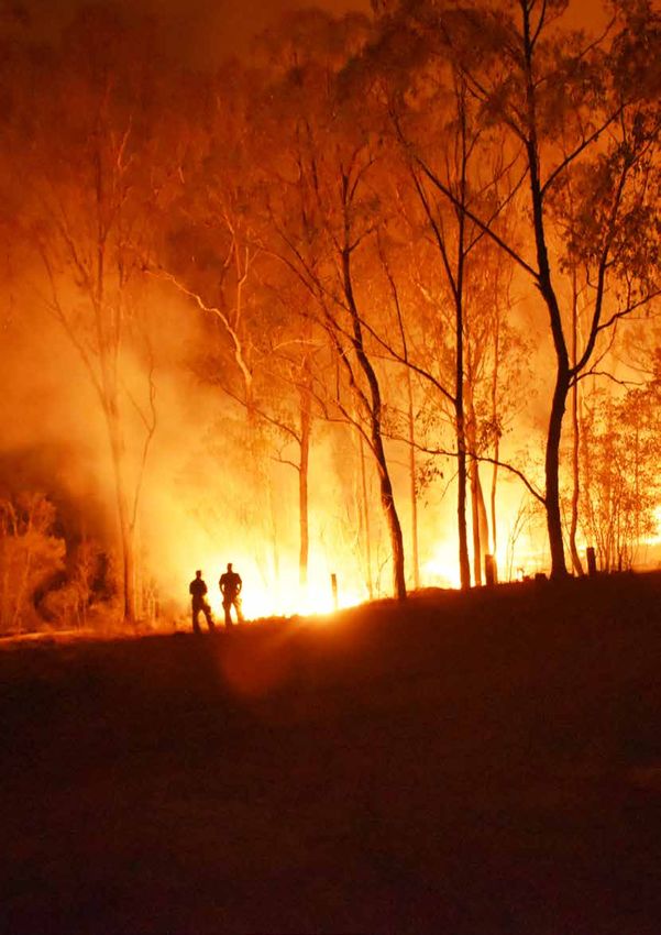
WMO-No. 1248
© World Meteorological Organization, 2020
The right of publication in print, electronic and any other form and in any language is reserved by WMO.
Short extracts from WMO publications may be reproduced without authorization, provided that the complete source
is clearly indicated. Editorial correspondence and requests to publish, reproduce or translate this publication in
part or in whole should be addressed to:

Chair, Publications Board
World Meteorological Organization (WMO)
7 bis, avenue de la Paix                                              Tel.: +41 (0) 22 730 84 03
P.O. Box 2300                                                         Fax: +41 (0) 22 730 81 17
CH-1211 Geneva 2, Switzerland                                         Email: publications@wmo.int

ISBN 978-92-63-11248-4

Cover illustration: Volunteer firefighters rescuing lives and farms from bushfire in Bundaberg, Queensland (Australia).

NOTE

The designations employed in WMO publications and the presentation of material in this publication do not imply the expression of any opinion
whatsoever on the part of WMO concerning the legal status of any country, territory, city or area, or of its authorities, or concerning the delimitation
of its frontiers or boundaries.

The mention of specific companies or products does not imply that they are endorsed or recommended by WMO in preference to others of a similar
nature which are not mentioned or advertised.

The findings, interpretations and conclusions expressed in WMO publications with named authors are those of the authors alone and do not necessarily
reflect those of WMO or its Members.
Contents
Foreword .  .  .  .  .  .  .  .  .  .  .  .  .  .  .  .  .  .  .  .  .  .  .  .  .  .  .  .  .  .  .  .  .  .  .  .  .  .  .  .  .  .  .  .  .  .  . 3

Statement by the United Nations Secretary-General .  .  .  .  .  .  .  .  .  .  .  .  .  .  .  .  .  .  .  .  .  . 4

Key messages .  .  .  .  .  .  .  .  .  .  .  .  .  .  .  .  .  .  .  .  .  .  .  .  .  .  .  .  .  .  .  .  .  .  .  .  .  .  .  .  .  .  .  . 5

Global Climate Indicators .  .  .  .  .  .  .  .  .  .  .  .  .  .  .  .  .  .  .  .  .  .  .  .  .  .  .  .  .  .  .  .  .  .  .  .  .  . 6

    Temperature  .  .  .  .  .  .  .  .  .  .  .  .  .  .  .  .  .  .  .  .  .  .  .  .  .  .  .  .  .  .  .  .  .  .  .  .  .  .  .  .  .  .  . 6

    Greenhouse gases and ozone .  .  .  .  .  .  .  .  .  .  .  .  .  .  .  .  .  .  .  .  .  .  .  .  .  .  .  .  .  .  .  .  .  . 7

    Ocean  .  .  .  .  .  .  .  .  .  .  .  .  .  .  .  .  .  .  .  .  .  .  .  .  .  .  .  .  .  .  .  .  .  .  .  .  .  .  .  .  .  .  .  .  .  .  . 9

    Cryosphere  .  .  .  .  .  .  .  .  .  .  .  .  .  .  .  .  .  .  .  .  .  .  .  .  .  .  .  .  .  .  .  .  .  .  .  .  .  .  .  .  .  .  .  14

    Drivers of short-term climate variability .  .  .  .  .  .  .  .  .  .  .  .  .  .  .  .  .  .  .  .  .  .  .  .  .  .  .                       17

    High-impact events in 2019  .  .  .  .  .  .  .  .  .  .  .  .  .  .  .  .  .  .  .  .  .  .  .  .  .  .  .  .  .  .  .  .  .  .                18

Climate-related risks and impacts .  .  .  .  .  .  .  .  .  .  .  .  .  .  .  .  .  .  .  .  .  .  .  .  .  .  .  .  .  .  .  . 27
    Health at increasing risk  .  .  .  .  .  .  .  .  .  .  .  .  .  .  .  .  .  .  .  .  .  .  .  .  .  .  .  .  .  .  .  .  .  .  .  .  27

    Food security and population displacement continue to be adversely
    affected by climate variability and extreme weather  .  .  .  .  .  .  .  .  .  .  .  .  .  .  .  .  .  .  .  .  29

    Marine life and biodiversity threatened by the changing climate and extreme events .  .  32

    Case study: Severe climatic shocks lead to a deterioration of the food security
    situation and to population displacement in the Greater Horn of Africa in 2019  .  .  .  .  .                                                   33

Dataset references .  .  .  .  .  .  .  .  .  .  .  .  .  .  .  .  .  .  .  .  .  .  .  .  .  .  .  .  .  .  .  .  .  .  .  .  .  .  .  .  . 35

List of contributors  .  .  .  .  .  .  .  .  .  .  .  .  .  .  .  .  .  .  .  .  .  .  .  .  .  .  .  .  .  .  .  .  .  .  .  .  .  .  .  .        39
Since 2016, the following United Nations agencies have significantly contributed to the
WMO Statement on the State of the Global Climate in support of climate policy and action:

    Food and Agriculture Organization of the United Nations (FAO),

    Intergovernmental Oceanographic Commission of the United Nations Educational,
    Scientific and Cultural Organization (IOC/UNESCO),

    International Monetary Fund (IMF),

    International Organization for Migration (IOM),

    United Nations Conference on Trade and Development (UNCTAD),

    United Nations Environment Programme (UNEP),

    Office of the United Nations High Commissioner for Refugees (UNHCR),

    United Nations Office for Disaster Risk Reduction (UNDRR),

    World Health Organisation (WHO).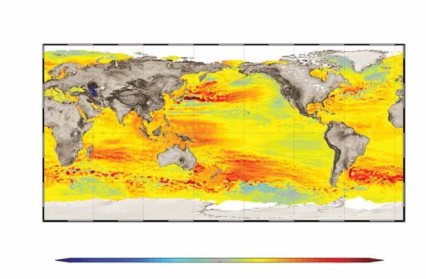
Foreword
                                                    Besides these powerful phenomena, there
                                                    has been weather-related damage, such
                                                    as the effects of multi-annual droughts on
                                                    the internal and cross-border migration of
                                                    populations, greater exposure of the world
                                                    population to health hazards due to heat and
                                                    pollution, and the reduction of economic
                                                    growth, especially in developing economies,
                                                    due to rising temperatures and weather
                                                    extremes.

                                                    The results of this report demonstrate that
                                                    climate change is already very visible in various
                                                    ways. More ambitious climate mitigation
                                                    efforts are needed to keep the warming below
                                                    2 °C by the end of the century.

Concentrations of greenhouse gases,                 The World Meteorological Organization will
particularly CO2, continue to rise. The year 2019   continue to follow closely climate variability
ended with a global average temperature of          and change and their impact. An information
1.1 °C above estimated pre-industrial averages,     portal is being set up to allow indicators of
second only to the record set in 2016. Without      the state of the climate to be tracked.
the role of El Niño in the warming increase
observed in 2016, 2019 would have been a            I would like to thank the many expert teams
record year.                                        in climatology and other disciplines, National
                                                    Meteorological and Hydrological Services, the
Temperature is one indicator of the ongoing         global and regional centres for climate data
climate change. Also, sea levels are rising at      collection and analysis and the United Nations
an increasing pace, through greater warming         sister agencies. Thanks to their unfailing
of the oceans, on the surface and in the            collaboration, the WMO Statement on the
depths, and through the enhanced melting            State of the Global Climate has become a
of Greenland’s ice and of glaciers, exposing        flagship publication providing policymakers
coastal areas and islands to a greater risk of      all over the world with essential climate
flooding and the submersion of low-lying            information.
areas.

Furthermore, in 2019, heatwaves, combined
with long periods of drought, were linked to
wildfires of unprecedented size. This was the
case in Australia, where millions of hectares
were set ablaze, and in Siberia and other Arctic                      (P. Taalas)
regions hit by wildfires of record intensity.                     Secretary-General

                                                                                                        3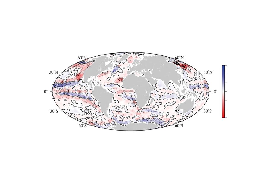
Statement by the United Nations
    Secretary-General
                                                       We are currently way off track to meeting
                                                       either the 1.5 °C or 2 °C targets that the Paris
                                                       Agreement calls for. We need to reduce
                                                       greenhouse gas emissions by 45% from 2010
                                                       levels by 2030 and reach net zero emissions by
                                                       2050. And for that, we need political will and
                                                       urgent action to set a different path.

                                                       This report outlines the latest science and
                                                       illustrates the urgency for far-reaching climate
                                                       action. It brings together data from across
                                                       the fields of climate science and lists the
                                                       potential future impacts of climate change
                                                       – from health and economic consequences
                                                       to decreased food security and increased
                                                       displacement.

    Climate change is the defining challenge of        I call on everyone – from government, civil
    our time. Time is fast running out for us to       society and business leaders to individual
    avert the worst impacts of climate disruption      citizens – to heed these facts and take urgent
    and protect our societies from the inevitable      action to halt the worst effects of climate
    impacts to come.                                   change. We need more ambition on mitigation,
                                                       adaptation and finance in time for the climate
    Science tells us that, even if we are successful   conference (COP26) to be held in Glasgow in
    in limiting warming to 1.5 °C, we will face        November. That is the only way to ensure a
    significantly increased risks to natural and       safer, more prosperous and sustainable future
    human systems. Yet, the data in this report        for all people on a healthy planet.
    show that 2019 was already 1.1 °C warmer
    than the pre-industrial era. The consequences
    are already apparent. More severe and
    frequent floods, droughts and tropical storms,
    dangerous heatwaves and rising sea levels
    are already severely threatening lives and                        (A. Guterres)
    livelihoods across the planet.                          United Nations Secretary-General

4
Key messages                                                                    The global mean temperature
                                                                                    for 2019 was 1.1±0.1 °C above
                                                                                pre-industrial levels. The year 2019 is
                                                                               likely to have been the second warmest
                                                                                 in instrumental records. The past five
                                                                                 years are the five warmest on record,
                                                                                  and the past decade, 2010–2019, is
                                                                                 also the warmest on record. Since the
                      Global atmospheric mole fractions                        1980s, each successive decade has been
                     of greenhouse gases reached record                             warmer than any preceding one
                   levels in 2018 with carbon dioxide (CO2)                                   since 1850.
                      at 407.8±0.1 parts per million (ppm),
                  methane (CH4) at 1869±2 parts per billion
                  (ppb) and nitrous oxide (N2O) at 331.1±0.1
                  ppb. These values constitute, respectively,
                    147%, 259% and 123% of pre-industrial
                     levels. Early indications show that the          The year 2019 saw low sea-ice
                     rise in all three – CO2, CH4 and N2O –            extent in both the Arctic and
                                 continued in 2019.               the Antarctic. The daily Arctic sea-ice
                                                                   extent minimum in September 2019
                                                                   was the second lowest in the satellite
                                                                     record. In Antarctica, variability in
                                                                   recent years has been high with the
                                                                    long-term increase offset by a large
                                                                   drop in extent in late 2016. Extents
                                                                    have since remained low, and 2019
 The ocean absorbs around 90% of                                      saw record-low extents in some
the heat that is trapped in the Earth                                             months.
   system by rising concentrations
  of greenhouse gases. Ocean heat
  content, which is a measure of this
 heat accumulation, reached record-
       high levels again in 2019.

                                                                                  Over the decade 2009–2018,
                                                                               the ocean absorbed around 23% of
                                                                               the annual CO2 emissions, lessening
                                                                                    the increase in atmospheric
                                                                                   concentrations. However, CO2
                                                                                 absorbed in sea water decreases
                                                                                    its pH, a process called ocean
                                As the ocean warms it expands and             acidification. Observations from open-
                                   sea levels rise. This rise is further        ocean sources over the last 20 to 30
                                   increased by the melting of ice on         years show a clear decrease in average
                                  land, which then flows into the sea.         pH at a rate of 0.017–0.027 pH units
                               Sea level has increased throughout the             per decade since the late 1980s.
                               altimeter record, but recently sea level
                                 has risen at a higher rate due partly
                                 to increased melting of ice sheets in
                                  Greenland and Antarctica. In 2019,
                                the global mean sea level reached its
                                 highest value since the beginning of
                                 the high-precision altimetry record
                                            (January 1993).                                                   5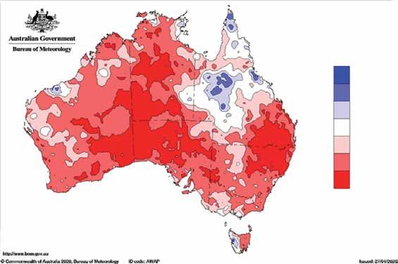
Global Climate Indicators
                                    Global Climate Indicators describe the                          TEMPERATURE
                                    changing climate, providing a broad picture
                                    of climate change at a global level that goes                   The global mean temperature for 2019 was
                                    beyond temperature. They provide important                      around 1.1 ± 0.1 °C above the 1850–1900
Figure 1. Global annual             information for the domains most relevant to                    baseline, used as an approximation of pre-
       mean temperature             climate change, including the composition of                    industrial levels. The year 2019 is likely
     difference from pre-           the atmosphere, the energy changes that arise                   to be the second warmest on record. The
    industrial conditions           from the accumulation of greenhouse gases and                   WMO assessment is based on five global
  (1850–1900). The two              other factors, and the responses of land, oceans                temperature datasets1 (Figure 1), with four of
        reanalyses (ERA5
                                    and ice. Key Global Climate Indicators include                  the five putting 2019 in second place and one
          and JRA-55) are
                                    global mean surface temperature, atmospheric                    dataset placing it third warmest. The spread
 aligned with the in situ
     datasets (HadCRUT,             greenhouse gas concentrations, ocean heat                       of the five estimates is between 1.05 °C and
 NOAAGlobalTemp and                 content, global sea level, ocean acidification,                 1.18 °C.
      GISTEMP) over the             sea-ice extent and the mass balance of glaciers
       period 1981–2010.            and ice sheets.                                                 The Intergovernmental Panel on Climate
                                                                                                    Change (IPCC) Special Report: Global Warming
                                                                                                    of 1.5 °C (IPCC SR15) concluded that “Human-
                                                                                                    induced warming2 reached approximately
      1.2          HadCRUT                                                                          1 °C (likely between 0.8 °C and 1.2 °C) above
                   NOAAGlobalTemp
                   GISTEMP
                                                                                                    pre-industrial levels in 2017, increasing at
      1.0
                   ERA5
                   JRA-55
                                                                                                    0.2 °C (likely between 0.1 °C and 0.3 °C) per
      0.8
                                                                                                    decade (high confidence)”. An update of the
      0.6                                                                                           figures for 2019 is consistent with continued
                                                                                                    warming in the range of 0.1–0.3 °C per decade.
°C

      0.4

      0.2
                                                                                                    The year 2016, which began with an
      0.0
                                                                                                    exceptionally strong El Niño, remains the
     –0.2                                                                                           warmest on record. Weak El Niño conditions
            1850          1875          1900     1925          1950     1975     2000     2025
                                                                                                    in the first half of 2019 may have made a small
                                                        Year                                        contribution to the high global temperatures

 Figure 2. Surface-air
   temperature anomaly
    for 2019 with respect
         to the 1981–2010
        average (Source:
     European Centre for
Medium-range Weather
     Forecasts (ECMWF)
 ERA5 data, Copernicus                                                         –10 –5 –3 –2 –1 –0.5 0 0.5 1    2   3   5 10 °C
                                                        Data source: ERA5
Climate Change Service)

                                    1
                                        The five datasets comprise three in situ datasets – HadCRUT.4.6.0.0 produced by the UK Met Office and the Climatic
                                        Research Unit at the University of East Anglia, NOAAGlobalTemp v5 produced by the US National Atmospheric and
                                        Oceanic Administration (NOAA), and GISTEMP v4 produced by the US National Aeronautics and Space Administration
                                        (NASA) Goddard Institute for Space Studies – as well as two reanalyses – ERA5 produced by the European Centre for
                                        Medium-range Weather Forecasts (ECMWF) for the Copernicus Climate Change Service, and JRA-55 produced by the
                                        Japan Meteorological Agency.
                                    2
                                        Total warming refers to the actual temperature change, irrespective of cause, while human-induced warming refers to the
                                        component of that warming that is attributable to human activities. The estimate of human-induced warming is based on:
                                        Haustein, K. et al., 2017: A real-time Global Warming Index. Scientific Reports 7, 15417, doi:10.1038/s41598-017-14828-5.

            6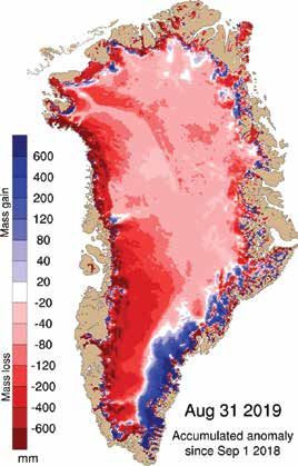
335
420 1900
410 330
1850
400
325
CO2 mole fraction (ppm)
N2O mole fraction (ppb)
1800
CH4 mole fraction (ppb)
390
320
380 1750
315
370
1700
310
360
1650
305
350
340 1600 300
1985 1990 1995 2000 2005 2010 2015 1985 1990 1995 2000 2005 2010 2015 1985 1990 1995 2000 2005 2010 2015
Year Year Year
20 2.0
4.0
15
1.5
3.0
N2O growth rate (ppb/yr)
CH4 growth rate (ppb/yr)
CO2 growth rate (ppm/yr)
10
1.0
2.0
5
0.5
1.0
0
0.0 –5 0.0
1985 1990 1995 2000 2005 2010 2015 1985 1990 1995 2000 2005 2010 2015 1985 1990 1995 2000 2005 2010 2015
Year Year Year
in 2019, but there was no clear increase in GREENHOUSE GASES AND OZONE Figure 3. Top row:
Globally averaged mole
temperature at the start of the year as was
fraction (measure of
seen in early 2016. Global averaged mole fractions of greenhouse concentration), from
gases are calculated from in situ observations 1984 to 2018, of CO 2 in
The past five years, 2015–2019, are the five at multiple sites, obtained through the Global parts per million (left),
warmest on record. The last five-year (2015– Atmosphere Watch (GAW) Programme of CH 4 in parts per billion
2019) and ten-year (2010–2019) averages are WMO. These data are available from the World (centre) and N 2 O in parts
also the warmest on record.3 Since the 1980s, Data Centre for Greenhouse Gases operated per billion (right). The
each successive decade has been warmer by the Japan Meteorological Agency.4 The red line is the monthly
mean mole fraction
than any preceding one since 1850. year 1750 is used as a representative baseline
with the seasonal
for pre-industrial conditions. variations removed; the
Although the overall warmth of the year is blue dots and line show
clear, there were variations in temperature Increasing levels of greenhouse gases in the the monthly averages.
anomalies across the globe. Most land areas atmosphere are a major driver of climate change. Bottom row: The growth
were warmer than the recent average (1981– Atmospheric concentrations reflect a balance rates representing
2010, Figure 2). The year 2019 was among between sources (including emissions) and increases in successive
the top three warmest on record since at sinks. Global CO2 concentrations reflect the annual means of mole
fractions for CO 2 in parts
least 1950 over Africa. Other continental balance between emissions due to human
per million per year
averages were among the three warmest, activities and uptake by the biosphere and ocean.
(left), CH 4 in parts per
except the average for North America, which billion per year (centre)
was nominally 14th warmest. The US State In 2018, greenhouse gas mole fractions reached and N 2 O in parts per
of Alaska was exceptionally warm. Areas of new highs, with globally averaged mole billion per year (right)
notable warmth for the year include large fractions of CO2 at 407.8±0.1 ppm, CH4 at 1869±2 (Source: WMO Global
areas of the Arctic, central and eastern ppb and N2O at 331.1±0.1 ppb (Figure 3). The Atmosphere Watch).
Europe, southern Africa, mainland south- annual increases in the three main greenhouse
east Asia, parts of Australia (where it was gases were larger than the increases in the
the warmest and the driest year on record), previous year and the 10-year averaged growth
north-east Asia and parts of Brazil. Outside rates. The global averaged mole fractions in
of North America, there were limited areas 2018 constitute, respectively, 147%, 259% and
of below-average temperature over land. 123% of pre-industrial (1750) levels.
3
For non-overlapping five- and ten-year periods.
4
https://gaw.kishou.go.jp/
7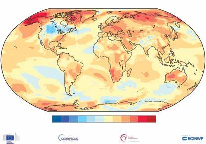
Global average figures for 2019 will not be                             were on average 34.7 ± 1.8 GtCO2 (billions of
                               available until late 2020, but real-time data                           tonnes) per year, growing at an average rate
                               from specific locations, including Mauna Loa                            of 0.9% per year to reach a record 36.6 GtCO2
                               (Hawaii) and Cape Grim (Tasmania) indicate                              in 2018. Carbon dioxide emissions from land
                               that levels of CO2, CH4 and N2O continued to                            use change were 5.5 ± 2.6 GtCO2 for the same
                               increase in 2019.                                                       period with no clear trend (Figure 4).

                               The IPCC SR15 report found that limiting                                In the 2009–2018 decade, both atmospheric
                               warming to 1.5 °C above pre-industrial levels                           CO 2 concentration and its grow th rate
                               implies reaching net zero CO 2 emissions                                increased, and land and ocean CO 2 sinks
                               globally around 2050 and concurrent deep                                continued to grow in response to the rise in
                               reductions in emissions of non-CO2 forcers,                             atmospheric CO2 concentrations. The land
                               particularly methane.                                                   and ocean CO2 sinks remove about 45% of all
                                                                                                       anthropogenic CO2 emissions. A preliminary
                               CARBON BUDGET                                                           projection of global fossil CO2 emissions, using
                                                                                                       data from the first three quarters of 2019,
                               Accurate assessment of anthropogenic CO2                                suggested that emissions would grow 0.6%
                               emissions and their redistribution among the                            in 2019, with a range of -0.2% to +1.5% that
                               atmosphere, ocean and terrestrial biosphere                             includes the possibility of no growth or even
                               – the “global carbon budget”5 – is important                            slight decline in emissions relative to 2018.
                               to better understand the global carbon cycle,                           Fire emissions in deforestation zones indicate
                               support the development of climate policies,                            that emissions from land use change for 2019
                               and project future climate change.                                      were above the 2009–2018 average. In 2019,
                                                                                                       the growth rate in atmospheric CO2 was 19.1 ±
                               Fossil CO2 emissions have increased steadily                            3.3 GtCO2, above the 2009–2018 average, with
                               over the past two centuries, with brief                                 the increase driven by rising CO2 emissions.
                               interruptions due to minor falls associated                             The preliminary estimates for the ocean and
                               with major economic downturns such as                                   land CO2 sink in 2019 were 9.5 GtCO2 and 14.3
                               recessions or oil price shocks. Over the                                GtCO2 respectively, both above their decadal
                               2009–2018 decade, for which complete data                               average.
                               are available, global fossil CO 2 emissions

 Figure 4. Perturbation
       budget of the global
  carbon cycle as a result
       of human activities,
      averaged globally for
   the decade 2009–2018.
                                              Fossil CO2      Land-use change       Biosphere          Atmospheric CO2        Ocean
         The anthropogenic                                                                                                                      Anthropogenic fluxes,
                                                                                                                                                2009–2018 average
   perturbation occurs on                                                                                                                       GtCO2 per year
      top of natural carbon                                         6                                      +18
    fluxes, with fluxes and                                       (3–8)                                                         9             Carbon cycling,
                                                                                                                                              GtCO2 per year
                                                                                        12                                    (7–11)
        stocks represented           0.5                                                                                                      Stocks
                                                                                       (9–14)
          by thinner arrows
                                                35                  440
            and circles. The                 (33–37)
       imbalance between
        total emissions and                                                                                                            330
                                                                          Vegetation
    total sinks reflects the                                     440                                                                                   Dissolved
                                           Gas reserves
   gaps in data, modelling                                                                                                                         inorganic carbon
                                                                                                                                    330
      or our understanding                                 Permafrost              Rivers                          Organic carbon            Marine
        of the carbon cycle                 Oil reserves                  Soils   and lakes                                                  biota
                                                                                              Coasts
 (Sources: Global Carbon                                                                                    Surface
      Project, http://www.                                                                                 sediments

globalcarbonproject.org/                   Coal reserves
                                                                                        Budget imbalance +2
             carbonbudget;
Friedlingstein et al. 2019).

                               5
                                   Friedlingstein, P. et al., 2019: Global Carbon Budget 2019. Earth System Science Data, 11, 1783–1838, https://www.earth-
                                   syst-sci-data.net/11/1783/2019/.

        8
Ozone hole area – Southern hemisphere
STRATOSPHERIC OZONE AND OZONE 30
DEPLETING GASES
25
Following the success of the Montreal Protocol,
the use of halons and chlorofluorocarbons
Area [million km2]
(CFCs) has been reported as discontinued. 20
Their levels in the atmosphere are monitored
to understand the continued effect they have
15
on the ozone layer and to detect unexpected
changes. Recent studies reported a slowdown
in the decline of the atmospheric concentration 10
of CFC-11 after 2012,6 connecting it to an increase
in global emissions to which emissions from
5
eastern Asia contributed. Because of their long
atmospheric lifetime, these compounds will
remain in the atmosphere for many decades. 0
Even if there were no new emissions, there Jul. Aug. Sept. Oct. Nov. Dec.
is more than enough chlorine and bromine Months
present in the atmosphere to cause complete
destruction of ozone at certain altitudes content is a measure of global warming, as Figure 5. Area
in Antarctica from August to December. it represents a large proportion of the heat (millions of km 2 ) where
Consequently, the formation of the ozone accumulating in the climate system. Thermal the total ozone column
is less than 220 Dobson
hole continues to be an annual spring event expansion from ocean warming, combined
units; 2019 is shown in
with year to year variation in its size and depth with melting of ice on land, leads to sea level
red. The most recent
largely governed by meteorological conditions. rise, which affects coastal areas. Changes in years are shown for
ocean chemistry associated with rising CO2 comparison as indicated
The 2019 ozone hole developed relatively concentrations in the atmosphere are altering by the legend. The
early and continued growing until a sudden the pH of the oceans. smooth, thick grey line is
stratospheric warming in September disturbed the 1979–2018 average.
the progression of the ozone destruction and OCEAN HEAT CONTENT The blue shaded area
represents the 30th to
led to the ozone hole being smaller and weaker
70th percentiles, and
than the long-term mean. The area of ozone Ocean heat content (OHC) is a fundamental
the green shaded area
depletion was below the long-term mean and metric for climate change as it is a measure represents the 10th and
the minimum ozone remained above the long- of heat accumulation in the Earth system. 90th percentiles for the
term mean until the beginning of November, Human-induced atmospheric composition period 1979–2018. The
several weeks earlier than usual. The ozone changes cause a radiative imbalance at the top thin black lines show the
hole area reached its maximum for 2019 on of the atmosphere – Earth’s energy imbalance maximum and minimum
8 September, with 16.4 million km2. By way – which is driving global warming.7 Due to values for each day in
of comparison, it reached 29.9 million km2 on the ocean’s large heat capacity, the majority the 1979–2018 period.
The plot is made at
9 September 2000 and 29.6 million km2 on (~90%) of this accumulated heat is stored in
WMO on the basis of
24 September 2006, according to an analysis the global ocean. data downloaded from
from the US National Aeronautics and Space the NASA Ozone Watch
Administration (NASA) (Figure 5). Consequently, the ocean is warming, (https://ozonewatch.
with wide-reaching impacts on the Earth gsfc.nasa.gov/). The
climate system. For example, OHC increase NASA data are based on
OCEAN contributes more than 30% of observed global satellite observations
mean sea-level rise through thermal expansion from the OMI and TOMS
instruments.
The ocean is an important part of the Earth of sea water. 8 Ocean warming is altering
system. The rate of change in ocean heat ocean currents9,10 and indirectly altering storm
6
Montzka, S. A. et al., 2018: An unexpected and persistent increase in global emissions of ozone-depleting CFC 11. Nature,
557:413–417, doi:10.1038/s41586-018-0106-2.
7
Hansen, J.et al., 2011: Earth’s energy imbalance and implications. Atmospheric Chemistry and Physics, 11, 13 421–13 449.
8
World Climate Research Programme (WCRP) Global Sea Level Budget Group, 2018: Global sea-level budget 1993–present.
Earth System Science Data, 10, 1551–1590, https://doi.org/10.5194/essd-10-1551-2018.
9
Hoegh-Guldberg, O. et al., 2018: Impacts of 1.5 ºC Global Warming on Natural and Human Systems. In: Intergovernmental
Panel on Climate Change (IPCC), 2018: Global Warming of 1.5 °C (Masson-Delmotte, V., P. Zhai, H.-O. Pörtner, D. Roberts,
J. Skea, P.R. Shukla, A. Pirani, W. Moufouma-Okia, C. Péan, R. Pidcock, S. Connors, J.B.R. Matthews, Y. Chen, X. Zhou, 9
M.I. Gomis, E. Lonnoy, T. Maycock, M. Tignor, and T. Waterfield, eds.). Geneva.changes in behaviour (including reproduction)
(a) (b)
and redistribution of habitats.17,18,19
Ensemble mean
1.2
1.0
Historical measurements back to the 1940s
mostly relied on shipboard techniques, which
0.8 constrained the availability of subsurface
OHC trends
0.6
temperature observations at global scale
and at depth. 20 Global-scale estimates of
OHC are thus often limited to the period from
OHC (J/m2)
0.4
1960 onwards, and to a vertical integration
0.2
from the surface down to a depth of 700 m.
With the deployment of the Argo network of
Depth autonomous profiling floats, which reached
target coverage in 2006, it is now possible
to routinely measure OHC changes down to
a depth of 2000 m21 (Figure 6).
Year
In 2019, OHC in the upper 700 m (a series of
measurements starting in the 1950s) and in
the upper 2000 m (a series of measurements
Figure 6. (a) Near- tracks.11,12 The implications of ocean warming starting in 2006) continued to rise reaching
global (60° S–60° N) area are widespread across Earth’s cryosphere record or near-record levels, with the average
averaged OHC over the too, as floating ice shelves become thinner for the year exceeding the previous record
period 1960–2018 and as
and ice sheets retreat.13,14,15,16 Ocean warming highs set in 2018. In the last quarter of the
derived from different
subsurface temperature
increases ocean stratification and, together decade and compared to the historical heat
products. Argo-based with ocean acidification and deoxygenation, uptake since 1960, global ocean heat gain
products have been can lead to dramatic changes in ecosystem has increased in the upper (0–700 m) layer,
superimposed from the assemblages and biodiversity, to population and heat has been sequestered in the deeper
year 2005 onwards as extinction, coral bleaching, infectious diseases, ocean layers (0–2000 m).
indicated in the legend; 22
(b) Rate of change of the
ensemble mean of OHC
10
Rhein, M.et al., 2018: Greenland submarine meltwater observed in the Labrador and Irminger Seas. Geophysical Research
Letters, 45, https://doi.org/10.1029/2018GL079110.
time series shown in (a),
together with its ensemble
11
Yang, H. et al., 2016: Intensification and poleward shift of subtropical western boundary currents in a warming climate.
spread. Rates amount to Journal of Geophysical Research: Oceans, 121, 4928–4945, doi:10.1002/2015JC011513.
0.3±0.1 Wm -2 (0–700 m, 12
Woollings, T. et al., 2012: Response of the North Atlantic storm track to climate change shaped by ocean - atmosphere
1960–2018), 0.6±0.1 Wm -2 coupling. Nature Geoscience, May 2012, doi: 10.1038/NGEO1438.
(0–700 m, 2005–2018), 13
Shi, J. R. et al., 2018: Evolving relative importance of the Southern Ocean and North Atlantic in anthropogenic ocean
1.0±0.1 Wm -2 (0–2000 m, heat uptake. Journal of Climate, 31, 7459--7479, https://doi.org/10.1175/JCLI-D-18-0170.1.
2005–2018). 14
Polyakov, I. V. et al., 2017: Greater role for Atlantic inflows on sea-ice loss in the Eurasian basin of the Arctic ocean.
Science, 356, 285-291, doi: 10.1126/science.aai8204.
15
Straneo, F. et al., 2019: The case for a sustained Greenland Ice sheet - Ocean Observing System (GrIOOS). Frontiers in
Marine Science, 6, 138, doi: 10.3389/fmars.2019.00138.
16
Shepherd, A. et al., 2018: Trends and connections across the Antarctic cryosphere. Nature, 558(7709), pp. 223-232,
https://doi.org/10.1038/s41586-018-0171-6.
17
Gattuso, J-P. et al., 2015: Contrasting futures for ocean and society from different anthropogenic CO 2 emissions scenarios.
Science, 349, 6243, doi: 10.1126/science.aac4722.
18
Molinos, J.G. et al., 2016: Climate velocity and the future global redistribution of marine biodiversity. Nature Climate
Change, 6, https://doi.org/10.1038/nclimate2769.
19
Ramírez, F. et al., 2017: Climate impacts on global hot spots of marine biodiversity. Science Advances, 3(2), doi: 10.1126/
sciadv.1601198.
20
Abraham, J. P. et al., 2013: A review of global ocean temperature observations: implications for ocean heat content
estimates and climate change. Review of Geophysics, 51, 450–483, doi: 10.1002/rog.20022.
21
Riser, S. et al., 2016: Fifteen years of ocean observations with the global Argo array. Nature Climate Change, 6, 145–153,
https://doi.org/10.1038/nclimate2872.
22
More information on the different data products used can be found in the references mentioned in the legend; for CARS2009,
further information is available at http://www.marine.csiro.au/~dunn/cars2009/), for the International Pacific Research
Centre (IPRC) at http://apdrc.soest.hawaii.edu/projects/argo/, and for the Copernicus Marine Service at http://marine.
copernicus.eu/.
10MARINE HEATWAVES MHW categories of 2019
NOAA OISST; Climatology period: 1982–2011
(a)
As with heatwaves on land, extreme heat can
affect the near-surface layer of the oceans
with a range of consequences for marine
life and dependent communities. Satellite
retrievals of sea-surface temperature can be
used to monitor marine heatwaves (MHWs).
In this case, MHWs are categorized as follows:
moderate, when the sea-surface temperature is
above the 90th percentile of the climatological (b) 100% (c) 100% (d)
distribution for five days or longer;23 strong,
50
90% 90%
80% 80%
Average MHW category per pixel
40
if the difference from the long-term average
Top MHW category per pixel
70% 70%
Global MHW count
(non-cumulative)
60% 60%
(cumulative)
30
(cumulative)
is more than twice that between the 90th
50% 50%
40% 40% 20
percentile and the long-term mean; severe, if
30% 30%
20% 20% 10
the difference from the long-term average is
10% 10%
0% 0% 0
2019–02 2019-04 2019-06 2019-08 2019-10 2019-12 2019–02 2019-04 2019-06 2019-08 2019-10 2019-12 2019–02 2019-04 2019-06 2019-08 2019-10 2019-12
Day of the year Day of first occurrence Day of the year
more than three times as large, and extreme, if Category: I Moderate II Strong III Severe IV Extreme
that difference is more than four times as large.
For 2019 (Figure 7), the number of MHW associated with extensive mortality of key Figure 7. (a) Global
days averaged over the entire ocean was marine habitat-forming communities along map showing the
approximately 55 days per pixel, nearly more than 45% of Australia’s continental highest MHW category
experienced at each
2 months of unusually warm temperatures. coastline, between 2011 and 2017. 28
pixel over the course
More of the ocean had an MHW classified as of the year, estimated
strong (41%) rather than moderate (29%), and SEA LEVEL using the NOAA OISST
84% of the ocean experienced at least one v2 dataset (reference
MHW. In large areas of the north-east Pacific, In 2019, the sea level continued to rise period 1982–2011).
MHWs reached the “severe” category. From (Figure 8, left), with the global mean sea White indicates that
2014 to 2016, sea-surface temperatures in the level reaching its highest value since the no MHWs occurred in
area were also unusually high and the mass beginning of the high-precision altimetry a pixel over the entire
year; (b) Stacked bar plot
of warmer than average waters was dubbed record (January 1993). The average rate of
showing the percentage
the “blob”. 24,25 Another notable area is the rise is estimated at 3.24 ± 0.3 mm yr –1 over of ocean pixels
Tasman Sea, where there has been a series the 27 year period, but the rate has increased experiencing an MHW
of MHWs in the summers of 2015/2016, 26 over that time. A greater loss of ice mass on any given day of the
2017/201827 and again in 2018/2019. In late from the ice sheets is the main cause of the year; (c) Stacked bar plot
2019, an extreme MHW also affected the accelerated rise in the global mean sea level8 showing the cumulative
area to the east of New Zealand. Climate on top of steady increases from the expansion percentage of the ocean
events, including MHWs and floods, were of ocean waters driven by warming. that experienced an
MHW over the year. 29
Horizontal lines in this
figure show the final
23
Hobday, A.J. et al., 2018 : Categorizing and naming marine heatwaves. Oceanography 31(2), https://doi.org/10.5670/
percentages for each
oceanog.2018.205.
category of MHW;
24
Gentemann, C. L. et al., 2017: Satellite sea surface temperatures along the West Coast of the United States during the (d) Stacked bar plot
2014–2016 northeast Pacific marine heat wave. Geophysical Research Letters, 44, 312– 319, doi:10.1002/2016GL071039. showing the cumulative
25
Di Lorenzo, E. and N. Mantua, 2016: Multi-year persistence of the 2014/15 North Pacific marine heatwave. Nature Climate number of MHW days
Change, 6(11), p.1042, doi: 10.1038/nclimate308. averaged over all pixels
26
Oliver, E.C. et al., 2017. The unprecedented 2015/16 Tasman Sea marine heatwave. Nature communications, 8, p.16101, in the ocean 30 (Source:
doi: 10.1038/ncomms16101. Robert Schlegel, Woods
27
Perkins-Kirkpatrick, S.E. et al., 2019: The role of natural variability and anthropogenic climate change in the 2017/18 Tasman Hole).
Sea marine heatwave. Bulletin of the American Meteorological Society, 100(1), pp.S105-S110, https://doi.org/10.1175/
BAMS-D-18-0116.1.
28
Babcock, R. C. et al., 2019: Severe continental-scale impacts of climate change are happening now: Extreme climate
events impact marine habitat forming communities along 45% of Australia’s coast. Frontiers in Marine Science, 6, https://
doi.org/10.3389/fmars.2019.00411.
29
These values are based on when in the year a pixel first experiences its highest MHW category, so no pixel is counted more
than once.
30
This is taken by finding the cumulative MHW days per pixel for the entire ocean and dividing that by the overall number of
ocean pixels (~690 000).
11Figure 8. Left: 100 8
Global mean sea-level 90
ESA Climate Change Initiative (SL_cci) data
CMEMS
evolution for January Near-real time Jason-3 6
80
1993–December 2019, Average trend: 3.24 +/– 0.3 mm/yr
4
from high-precision 70
2
altimetry. The thin black 60
Sea level (mm)
curve is a quadratic
Sea level (mm)
50
0
function that best fits 40 –2
the data. The data from
30
the Copernicus Marine –4
Environment Monitoring 20
–6
Service (CMEMS) 10
begin in January 2016 0
–8
and those from the –10 –10
1993 1996 1999 2002 2005 2008 2011 2014 2017 2020
European Organization
1993 1995 1997 1999 2001 2003 2005 2007 2009 2011 2013 2015 2017 2019
Time (yr) Time (yr)
for the Exploitation
of Meteorological
Satellites (EUMETSAT) Interannual variability (Figure 8, right) in sea-level trends in the southern hemisphere are east of
Jason-3 in October rise is mainly driven by the El Niño-Southern Madagascar in the Indian Ocean, east of New
2019. Right: Detrended Oscillation (ENSO, see also the section Drivers Zealand in the Pacific Ocean, and east of Rio de
global mean sea level of short-term climate variability). During El la Plata/South America in the South Atlantic.
over the same period
Niño, water from tropical river basins on land is In the northern hemisphere, an eastward,
(the difference between
transferred to the ocean by shifts in precipitation elongated pattern is also seen in the North
the smooth quadratic
function and the and run-off (as was the case in 1997, 2012 and Pacific. A previously strong pattern seen in
measured values in the 2015). During La Niña, the opposite occurs, with the western tropical Pacific over the first two
left panel). a transfer of water from the ocean to land (for decades of the altimetry record is now fading,
example, in 2011).31 suggesting that it was not a long-term signal.
Non-uniform sea-level trends are dominated
Sea-level rise is not regionally uniform. Figure 9 by geographical variations in OHC32,33 but also
shows the spatial trend patterns from January depend on processes involving the atmosphere,
1993 to May 2019. The strongest regional geosphere and cryosphere.
Regional mean sea level trends (January 1993–May 2019)
50° N
0° S
Figure 9. Regional
variability in sea-level
trends 1993–2019 based
on satellite altimetry
50° S
(Source: Copernicus/
Collecte Localisation
Satellites (CLS)/Centre
national d’études
50° E 100° E 150° E 160° W 110° W 60° W 10° W
spatiales (CNES)/
Laboratoire d’Études
en Géophysique et Data type: Obervations
(mm/year)
Océanographie Spatiales
–10.00 –6.67 –3.33 0.00 3.33 6.67 10.00
(LEGOS)).
31
Fasullo, J. T. et al., 2013: Australia’s unique influence on global sea level in 2010–2011. Geophysical Research Letters,
40, 4368–4373, doi:10.1002/grl.50834.
32
Church, J. A. et al., 2013: Sea Level Change. In: Intergovernmental Panel on Climate Change (IPCC), 2013: Climate Change
2013: The Physical Science Basis. Contribution of Working Group I to the Fifth Assessment Report of the Intergovernmental
12 Panel on Climate Change (Stocker, T. F. et al., (eds.)]. Cambridge and New York, Cambridge University Press.OCEAN ACIDIFICATION are more difficult to distinguish, due to the
complexity of the environment and the variety
In the decade 2009–2018, the ocean absorbed of influences on it. These changes affect
around 23% of annual CO2 emissions,34 which ocean services that are centred on the coast,
helps to alleviate the impact of climate which are important for human well-being,
change. However, increasing atmospheric such as fisheries and aquaculture, tourism
CO2 concentrations alter the chemistry of the and recreation. Strong seasonal patterns
ocean as CO2 reacts with seawater decreasing and variability in pH are evident in recent
its pH and increasing the acidity of the ocean. monitoring efforts in the Southern Ocean
This process is called ocean acidification. around New Zealand (Figure 10), highlighting
The change in pH is linked to other shifts the need for sustained long-term observations
in carbonate chemistry that decrease the with high temporal and spatial resolution.
ability of some marine organisms – such as
mussels, crustacean and corals – to calcify. The DEOXYGENATION
combined changes affect marine life, lessening
the potential for growth and reproduction. Both observations and numerical models
Observations from open-ocean sources over indicate that oxygen is declining in the
the last 20 to 30 years show a clear decrease modern open and coastal oceans, including
in average pH, with a decline of the average estuaries and semi-enclosed seas. Since the
global surface ocean pH of 0.017–0.027 pH middle of the last century, there has been an
units per decade since the late 1980s. estimated 1%–2% decrease (that is, 2.4–4.8
Pmol or 77 billion–145 billion tons) in the
In coastal seas, changes in carbonate chemistry global ocean oxygen inventory.35,36 However,
caused by anthropogenic ocean acidification ocean observations at 200-m depths show
Figure 10.
Auckland Wellington Harbour Measurements of
8.2 8.2
pH from four sites
8.15 8.15 around New Zealand,
8.1 8.1 spanning four to five
8 8
years of observations.
Top row: Urbanized
pHTOT
pHTOT
7.95 7.95
sites in Auckland and
7.9 7.9 Wellington. Bottom
7.85 7.85
row: One open coast
(Jackson Bay) and one
7.8 7.8
2015 2016 2017 2018 2019 2020 2015 2016 2017 2018 2019 2020 bay (Tasman Bay) site.
Year Year Seasonal patterns and
variability between
Jackson Bay Tasman Bay
8.2 8.2 pH measurements are
clearly visible (Credit:
8.15 8.15
Kim Currie, National
8.1 8.1 Institute of Water and
8 8 Atmospheric Research
(NIWA)).
pHTOT
pHTOT
7.95 7.95
7.9 7.9
7.85 7.85
7.8 7.8
2015 2016 2017 2018 2019 2020 2015 2016 2017 2018 2019 2020
Year Year
33
Intergovernmental Panel on Climate Change (IPCC), 2019: IPCC Special Report on the Ocean and Cryosphere in a Changing
Climate (H.-O. Pörtner, D.C. Roberts, V. Masson-Delmotte, P. Zhai, M. Tignor, E. Poloczanska, K. Mintenbeck, M. Nicolai,
A. Okem, J. Petzold, B. Rama, N. Weyer (eds.)). In press.
34
World Meteorological Organization (WMO), 2019: WMO Greenhouse Gas Bulletin: The State of Greenhouse Gases in the
Atmosphere. Based on Global Observations through 2018 , https://library.wmo.int/doc_num.php?explnum_id=10100.
35
Bopp, L. et al., 2013: Multiple stressors of ocean ecosystems in the 21st century: Projections with CMIP5 models. Biogeo-
sciences, 10:6225–6245, https://doi.org/10.5194/bg-10-6225-2013.
1330
Dissolved O2 difference (μmol kg–1)
20
10
0
10
–20
–30
Figure 11. Dissolved that changes vary across the ocean basins, like sea ice extent, have been measured from
oxygen difference with the highest loss of dissolved oxygen in space for many years, while the capability
between 2000–2018 and the northern hemisphere in the last decades to measure other components from space
1970–2018 using in situ
(Figure 11). is still developing. The major cryosphere
measurements in 200-m
seawater (bottle data),
indicators used here include sea-ice extent,
based on World Ocean The projected 7% expansion of the pre- glacier mass balance and the Greenland ice-
Atlas 2018 (Garcia et industrial area of oxygen minima (< 80 µmol sheet mass balance. Specific snow events are
al., 2018). kg-1) by 2100 is expected to alter the diversity, covered in the section High-impact events
composition, abundance and distribution of in 2019.
marine life. New studies further identified
deoxygenation alongside ocean warming and SEA ICE
ocean acidification as a major threat to ocean
ecosystems and human well-being. Even Arctic (as well as sub-Arctic) sea ice has seen
coral reefs are now recognized as vulnerable a long-term decline in all months during the
to major oxygen loss. 37 satellite era (1979–present, Figure 12), with
the largest relative losses in late summer,
around the time of the annual minimum in
CRYOSPHERE September, with regional variations.
The cryosphere includes solid precipitation, The 2019 Arctic winter maximum daily sea-
snow cover, sea ice, lake and river ice, ice extent (14.78 million km2), reached around
glaciers, ice caps, ice sheets, permafrost and 13 March, was the 7th lowest maximum on
seasonally-frozen ground. The cryosphere record, 38 and the March monthly average
provides key indicators of a changing climate, was also the 7 th lowest (Figure 12). The
yet it is one of the most under-sampled Arctic summer minimum daily sea-ice extent
domains of the Earth system. Many of the (4.15 million km2), which occurred around
components are measured at the surface, 18 September, was tied with 2007 and 2016 as
but spatial coverage is generally poor. Some, the second lowest on record.39 The September
36
Schmidtko, S. et al., 2017: Decline in global oceanic oxygen content during the past five decades. Nature, 542:335–339, doi:
10.1038/nature21399.
37
Camp E.F. et al., 2017: Reef-building corals thrive within hot-acidified and deoxygenated waters. Scientific Reports, 7(1),
2434, doi: 10.1038/s41598-017-02383-y.
38
http://nsidc.org/arcticseaicenews/2019/03/
39
http://nsidc.org/arcticseaicenews/2019/09/
14Figure 12. Monthly
September and March
1
Arctic sea-ice extent
anomalies (relative to
the 1981–2010 average)
0
for 1979– 2019 (Sources:
US National Snow and
Million km2
Ice Data Center (NSIDC)
–1
and EUMETSAT Ocean
and Sea Ice Satellite
Application Facility
–2
(OSI SAF))
NSIDC v3 (September)
NSIDC v3 (March)
OSI-SAF v2 (September)
–3 OSI-SAF v2 (March)
1980 1985 1990 1995 2000 2005 2010 2015
Year
monthly average extent was nominally the to normal in the northern part of this area,
3rd lowest on record.40 unlike the past decade when it was lower
than average. Winter 2018/2019 brought early
Extents remained very low till November, ice formation on the Great Lakes of North
with the ice edge advancing more slowly than America and above-average ice coverage. The
normal in the Beaufort, Chukchi, Kara and maximum ice coverage on the Great Lakes
Barents Seas. Around Svalbard, however, the was 145% of the long-term average and the
sea ice returned to near average conditions.41 7th highest since 1972/1973.42
From April to November 2019, monthly extents
were among the three lowest on record for Until 2016, Antarctic sea-ice extent had
those months, with the monthly extent for shown a small long-term increase (Figure 13).
October being the lowest on record. In late 2016, this was interrupted by a sudden
drop in extent to extremely low values. Since
Ice conditions varied considerably during the then, Antarctic sea-ice extent has remained at
2018/2019 winter in the Arctic regional seas. relatively low levels. The year 2019 saw three
Although ice extent was extremely low in months with record-low monthly extents
the Bering Sea, it was close to normal in the (May, June and July). Late austral winter and
adjacent Sea of Okhotsk. Northerly winds spring saw extents that were closer to the
in the Barents Sea region, from January to long-term average, but November had its 2nd
August 2019, meant that ice extent was close lowest extent on record, and December its
Jan.
Figure 13. Variability
Jan.
of seasonal patterns of
L, 1 000 km2
daily sea-ice extent for
Dec. L, 1 000 km2 Dec.
20 000
16 000
the Arctic (north of 45°
Nov. Nov.
Oct.
14 000
Oct.
N, left) and Antarctic
Sept. Sept. 15 000
(south of 50° S, right)
12 000
Aug. Aug.
calculated on the basis
July 10 000 July of the NSIDC NASA
Team series for 1978–
10 000
June June
2020 (Source: Arctic
8 000
May May
April
6 000 April
and Antarctic Research
5 000
Mar.
Institute (AARI))
Mar.
4 000
Febr.
Febr.
Jan.
Jan.
1980 1984 1988 1992 1996 2000 2004 2008 2012 2016 2020 1980 1984 1988 1992 1996 2000 2004 2008 2012 2016 2020
40
http://nsidc.org/arcticseaicenews/2019/10/
41
http://nsidc.org/arcticseaicenews/2019/11/
42
https://www.glerl.noaa.gov/data/ice/#historical
15Figure 14. Annual (blue) Global mass balance of WGMS reference glaciers
and cumulative (red) mass
balance of reference 5
glaciers with more than
Annual mass balance
30 years of ongoing 0
glaciological measurements.
Global mass balance is
Metre water equivalent
–5
based on an average for 19
regions to minimize bias
towards well-sampled –10
regions. Annual mass
changes are expressed in –15
meter water equivalent (m
Cumulative mass balance
w.e.) which corresponds to
–20
tonnes per square meter (1
000 kg m -2 ) (Source: World
Glacier Monitoring Service –25
1950 1960 1970 1980 1990 2000 2010 2020
(WGMS, 2020, updated). Year
4th or 5th lowest. The minimum daily sea-ice were lower than in the previous two years.
extent (2.47 million km2), reached around In late spring, snow cover on the glaciers
28 February, was the 7th lowest on record. was around 20% to 40% above normal and,
The maximum daily sea-ice extent (18.40 although the onset of melt was relatively late,
million km2) was reached around 30 September. the rate of loss reached record levels in late
June and early July during a two-week period
GLACIERS of intense heat. Melting continued until the
beginning of September. In the 12 months
Glaciers are formed from snow that has to October 2019, around 2% of Switzerland’s
compacted to form ice, which can deform total glacier volume was lost. Over the past
and flow downhill to lower, warmer altitudes, five years, the loss has exceeded 10%, the
where it melts or, if the glacier terminates in the highest rate of decline in more than a century
ocean, breaks up forming icebergs. Glaciers of records.
are sensitive to changes in temperature,
precipitation and incoming solar radiation GREENLAND ICE SHEET
as well as other factors such as changes in
basal lubrication or the loss of buttressing Changes in the mass of the Greenland ice
ice shelves. sheet reflect the combined effects of surface
mass balance (SMB) – defined as the difference
According to the World Glacier Monitoring between snowfall and run-off from the
Service, in the hydrological year 2017/2018, Greenland ice sheet, which is always positive
observed glaciers experienced an ice loss of at the end of the year – and mass losses at
0.89 metre water equivalent (m w.e.) (Figure 14). the periphery from the calving of icebergs
Preliminary results for 2019, based on a subset and the melting of glacier tongues that meet
of glaciers, indicate that the hydrological year the ocean.44
2018/2019 was the thirty-second consecutive
year of negative mass balance, with an ice The total ac cumulated SMB bet ween
loss in excess of 1 m w.e. Eight out of the ten September 2018 and August 2019 (Figure
most negative mass-balance years have been 15, left) was 169 Gt, which is the 7th lowest on
recorded since 2010. The cumulative loss of record. Nine of the 10 lowest SMB years since
ice since 1970 amounts to over 23 m w.e. 1981 have been observed in the last 13 years.
By way of comparison, the average SMB for
The year 2019 saw major losses in ice 1981–2010 is 368 Gt, and the lowest SMB
volume from Swiss glaciers, as reported by was 38 Gt in 2012. The surface mass balance
the Cryospheric Commission of the Swiss was below normal almost everywhere in
Academy of Sciences,43 though overall losses Greenland except the southeast (Figure 15,
43
https://naturalsciences.ch/organisations/ekk/118503-glacier-volume-reduced-by-10-per-cent-in-only-five-years
44
Based on the Polar Portal seasonal report for 2019 available at http://polarportal.dk/en/home/2019-season-report/.
1612
Mass gain 2018–2019
8
4
0
Gt/day
Mass loss
–4
–8
–12
SMB (Gt/day)
–16
Sept. Oct. Nov. Dec. Jan. Feb. Mar. Apr. May Jun. Jul. Aug.
Month
800
Mean (1981–2010)
2011_2012
600
2018–2019
400
Gt
200
0
Acc. SMB (Gt)
Sept. Oct. Nov. Dec. Jan. Feb. Mar. Apr. May Jun. Jul. Aug.
Month
right). This was due to a dry winter, a very DRIVERS OF SHORT-TERM CLIMATE Figure 15. Left: SMB
early start of the melting season and a long, VARIABILITY for the year 1 September
dry, warm summer. 2018 to 31 August
2019. The upper panel
The ocean plays several important roles in
shows individual days,
As noted earlier, SMB is always positive at the the climate. Surface temperatures change and the lower panel
end of the year, but the ice sheet also loses relatively slowly over the ocean so recurring the accumulated sum
ice through calving of icebergs and melting patterns in sea-surface temperature can be over the year. The year
where the glacier tongues meet warm sea used to understand and, in some cases, predict 2018/2019 is in blue, and
water. With satellites we can measure the the more rapidly changing patterns of weather the grey line is the long-
ice velocity of the outlet glaciers around the over land on seasonal time scales. Two factors, term average. By way of
edges of the ice sheet, and from that we can in particular, that can help to understand the comparison, the lower
panel shows the record
estimate how much ice is lost through calving climate of 2019, are the El Niño-Southern
year 2011/2012 in red.
and ocean melting. The analysis for 2018/2019 Oscillation and the Indian Ocean Dipole.
Units are gigatonnes (Gt)
gives a loss of about 498 Gt. In comparison, per day and gigatonnes,
the ice sheet lost an average of about 462 EL NIÑO-SOUTHERN OSCILLATION respectively. Right:
Gt per year as icebergs and through ocean Map showing SMB
melting over the period 1986–2018. The El Niño-Southern Oscillation (ENSO) is anomaly (in mm) across
one of the most important drivers of year-to- Greenland (Source:
Combining a gain in SMB of 169 Gt with ice loss year variability in global weather patterns. Polar Portal, http://
from calving and ocean melting of 498 Gt gives El Niño events, characterized by warmer polarportal.dk/en)
a net ice loss for 2018/2019 of 329 Gt. To put than average sea-surface temperatures in
this in context, data from the Gravity Recovery the eastern Pacific and a weakening of the
and Climate Experiment (GRACE) satellites trade winds, are associated with higher global
tell us that Greenland lost about 260 Gt of ice temperatures. Cooler global temperatures
per year over the period 2002–2016, with a often accompany La Niña events, which are
maximum of 458 Gt in 2011/2012. So, the 329 characterized by cooler than average sea-
Gt of this season is well above the average, surface temperatures in the eastern Pacific
but not a record loss. and a strengthening of the trade winds.
17Record global temperatures in 2016 followed HIGH-IMPACT EVENTS IN 2019
an unusually strong El Niño event in late 2015
and early 2016. In contrast, 2019 started with The following sections describe some of
neutral or weak El Niño conditions.45 Sea- the high-impact events that occurred in
surface temperatures reached or exceeded 2019. Information on such events is largely
typical El Niño thresholds from October based on contributions from WMO Members
2018 through the first half of 2019, but an with additional information from the Global
atmospheric response was absent in the Precipitation Climatology Centre (GPCC),
early stages of the event. Atmospheric Regional Climate Centres and tropical storm
indicators such as weakened trade winds monitoring centres.
and increased cloudiness at the dateline
did not show consistently until February. HEAT AND COLD WAVES
Thereafter, coupling between the ocean
and the atmosphere maintained sea-surface The year 2019 also saw numerous major
temperatures at borderline El Niño levels heatwaves. Amongst the most significant
until the middle of the year. were two heatwaves that occurred in Europe
in late June and late July (Figure 16). The
INDIAN OCEAN DIPOLE first one reached its maximum intensity in
southern France, where a national record of
The positive phase of the Indian Ocean 46.0 °C (1.9 °C above the previous record) was
Dipole (IOD) is characterized by cooler set on 28 June at Vérargues (Hérault). It also
than average sea-surface temperatures in affected much of western Europe. The second
the eastern Indian Ocean and warmer than one was more extensive, with national records
average sea-surface temperatures in the set in Germany (42.6 °C), the Netherlands
west. The negative phase has the opposite (40.7 °C), Belgium (41.8 °C), Luxembourg
pattern. The resulting change in the gradient (40.8 °C) and the United Kingdom (38.7 °C).
of sea-surface temperature across the ocean The heat also extended to the Nordic countries,
basin affects the weather of the surrounding where Helsinki had its highest temperature
continents. on record (33.2 °C) on 28 July. At some long-
term stations, records were broken by 2 °C or
In 2019, the IOD started weakly positive and more, including Paris, where a temperature of
became progressively more positive from 42.6 °C, at the main Montsouris observatory
May to October, ultimately becoming one on 25 July, was 2.2 °C above the previous
of the strongest positive IOD events since record set in 1947, and Uccle (near Brussels),
reliable records began around 1960. The IOD whose 39.7 °C was 3.1 °C above the previous
index declined somewhat before the end record (for impacts, see the section Extreme
of the year. The positive phase of the IOD heat and health).
during austral winter and spring has been
associated with drier and warmer conditions Japan experienced two heatwaves that were
over Indonesia and surrounding countries, as notable in different ways. The first occurred in
well as parts of Australia. Indeed, Australia late May, with unusually high temperatures,
has seen unusually dry conditions during including 39.5 °C (the equal highest on record
winter and spring exacerbating long-term for any time of year on the island of Hokkaido),
rainfall deficits. The positive IOD is also but limited impacts. The second, in July, was
linked to late withdrawal of the south-west less unusual in a meteorological sense but had
Indian monsoon, as was observed this year, much greater health impacts as it occurred
and to high rainfall in the later part of the during the peak of summer and was focused
year in east Africa. For more details on in the more heavily populated area of Honshu.
regional impacts, see the following sections:
Heavy rainfall and floods, Drought and Australia had an exceptionally hot summer in
Case study: Severe climatic shocks lead to 2018–2019. The mean summer temperature
a deterioration of the food security situation was the highest on record by almost 1 °C,
and to population displacement in the Greater and January was Australia’s hottest month
Horn of Africa in 2019. on record. Most of the country was affected,
45
http://www.wmo.int/pages/prog/wcp/wcasp/documents/WMO_ENSO_May19_Eng.pdf
18You can also read