Environment International - Contents lists available at ScienceDirect - Rrcap.ait.asia
←
→
Page content transcription
If your browser does not render page correctly, please read the page content below
Environment International 145 (2020) 106155
Contents lists available at ScienceDirect
Environment International
journal homepage: www.elsevier.com/locate/envint
Development of the Low Emissions Analysis Platform – Integrated Benefits
Calculator (LEAP-IBC) tool to assess air quality and climate co-benefits:
Application for Bangladesh
Johan C.I. Kuylenstierna a, Charles G. Heaps b, Tanvir Ahmed c, Harry W. Vallack a, W.
Kevin Hicks a, Mike R. Ashmore a, Christopher S. Malley a, *, Guozhong Wang a, Elsa N. Lefèvre d,
Susan C. Anenberg e, Forrest Lacey f, g, Drew T. Shindell h, Utpal Bhattacharjee i, Daven K. Henze f
a
Stockholm Environment Institute, Department of Environment and Geography, University of York, United Kingdom
b
US Center, Stockholm Environment Institute, Somerville, MA, United States
c
Department of Civil Engineering, Bangladesh University of Engineering and Technology, Dhaka, Bangladesh
d
Climate and Clean Air Coalition Secretariat, United Nations Environment Programme, Paris, France
e
Milken Institute, School of Public Health, George Washington University, Washington D.C., United States
f
Department of Mechanical Engineering, University of Colorado, Boulder, CO, United States
g
National Center for Atmospheric Research, Boulder, CO, United States
h
Nicholas School of the Environment, Duke University, Durham, NC, United States
i
Nature Conservation Management (NACOM), Dhaka, Bangladesh
A R T I C L E I N F O A B S T R A C T
Handling Editor: Dr. Hanna Boogaard Low- and middle-income countries have the largest health burdens associated with air pollution exposure, and
are particularly vulnerable to climate change impacts. Substantial opportunities have been identified to simul
Keywords: taneously improve air quality and mitigate climate change due to overlapping sources of greenhouse gas and air
Air pollution pollutant emissions and because a subset of pollutants, short-lived climate pollutants (SLCPs), directly contribute
Climate change
to both impacts. However, planners in low- and middle-income countries often lack practical tools to quantify the
Bangladesh
air pollution and climate change impacts of different policies and measures. This paper presents a modelling
Premature mortality
Fine particulate matter framework implemented in the Low Emissions Analysis Platform – Integrated Benefits Calculator (LEAP-IBC) tool
Scenario analysis to develop integrated strategies to improve air quality, human health and mitigate climate change. The frame
work estimates emissions of greenhouse gases, SLCPs and air pollutants for historical years, and future pro
jections for baseline and mitigation scenarios. These emissions are then used to quantify i) population-weighted
annual average ambient PM2.5 concentrations across the target country, ii) household PM2.5 exposure of different
population groups living in households cooking using different fuels/technologies and iii) radiative forcing from
all emissions. Health impacts (premature mortality) attributable to ambient and household PM2.5 exposure and
changes in global average temperature change are then estimated. This framework is applied in Bangladesh to
evaluate the air quality and climate change benefits from implementation of Bangladesh’s Nationally Determined
Contribution (NDC) and National Action Plan to reduce SLCPs. Results show that the measures included to
reduce GHGs in Bangladesh’s NDC also have substantial benefits for air quality and human health. Full imple
mentation of Bangladesh’s NDC, and National SLCP Plan would reduce carbon dioxide, methane, black carbon
and primary PM2.5 emissions by 25%, 34%, 46% and 45%, respectively in 2030 compared to a baseline scenario.
These emission reductions could reduce population-weighted ambient PM2.5 concentrations in Bangladesh by
18% in 2030, and avoid approximately 12,000 and 100,000 premature deaths attributable to ambient and
household PM2.5 exposures, respectively, in 2030. As countries are simultaneously planning to achieve the
climate goals in the Paris Agreement, improve air quality to reduce health impacts and achieve the Sustainable
Development Goals, the LEAP-IBC tool provides a practical framework by which planners can develop integrated
strategies, achieving multiple air quality and climate benefits.
* Corresponding author.
E-mail address: chris.malley@york.ac.uk (C.S. Malley).
https://doi.org/10.1016/j.envint.2020.106155
Received 12 June 2020; Received in revised form 17 September 2020; Accepted 21 September 2020
Available online 4 October 2020
0160-4120/© 2020 The Authors. Published by Elsevier Ltd. This is an open access article under the CC BY license (http://creativecommons.org/licenses/by/4.0/).
J.C.I. Kuylenstierna et al. Environment International 145 (2020) 106155
1. Introduction within LEAP. The results are displayed within LEAP’s graphical user
interface (GUI). While different tools exist to assess the impact of
Low- and middle- income countries (LMICs) are disproportionately different strategies on air pollution and climate change (Anenberg et al.,
affected by air pollution impacts on health, with millions of premature 2016; Kiesewetter et al., 2015; Van Dingenen et al., 2018), the overall
deaths attributed globally to exposure to outdoor (ambient) and tool (hereafter referred to as LEAP-IBC) has been specifically designed to
household particulate matter each year (Health Effects Institute, 2018). be accessible to planners in LMIC countries, in situations where data and
Climate change is affecting many countries with increasingly severe and institutional capacity for modelling are typically limited. This study
frequent heat waves, unusual levels of flooding and disruption of rainfall presents the analytical methodology within LEAP-IBC that allows for the
(Myles et al., 2018). These countries are least able to cope with the integrated assessment of the air quality and climate benefits of different
impacts of climate change, and air pollution places an additional burden mitigation measures, as well as overall strategies related to climate
on economic productivity, on the health system, and disproportionately mitigation, air quality management, energy planning, low emission
affects the poor, women and children. Countries have outlined their development, and sustainable development.
contribution to mitigating climate change through their Nationally The application of LEAP-IBC to assess integrated air pollution and
Determined Contributions (NDCs), which are currently not sufficient to climate change strategies in LMICs is illustrated for Bangladesh, where
achieve the global average temperature targets set out in the Paris there are significant air pollution health impacts (Goyal and Canning,
Agreement, and additional ambition is needed (Rogelj et al., 2016). 2017; Gurley et al., 2013; Khan et al., 2019; Shi et al., 1999), and vul
Some pollutants contribute to both poor air quality and climate change, nerabilities to climate change (Karim and Mimura, 2008; Ruane et al.,
while others share the same source (Fiore et al., 2015; von Schneide 2013). Two national strategies relevant for air pollution and climate
messer et al., 2015). Therefore, in the context of the increased ambition change are assessed. These are Bangladesh’s Nationally Determined
needed to meet global temperature goals, and the substantial burden air Contribution (NDC) that contains Bangladesh’s climate change
pollution has in LMICs, there is substantial potential for the develop commitment and the mitigation measures to achieve it (Ministry of
ment of integrated mitigation strategies in these countries to achieve Environment and Forests, 2015), and Bangladesh’s National Action Plan
simultaneous benefits for local air pollution and global climate change. to reduce SLCPs (Bangladesh Department of Environment, 2018).
The effectiveness of integrated air pollution and climate change Bangladesh was a founding member of the Climate and Clean Air Coa
strategies has been demonstrated by multiple global and regional as lition to reduce SLCPs (http://ccacoalition.org/), a voluntary partner
sessments. For example, the global implementation of actions targeting ship of over 120 State and non-State partners. With support from the
the major sources of Short-Lived Climate Pollutants (SLCPs), which CCAC Supporting National Action & Planning initiative, the Bangladesh
contribute to both air quality and climate impacts and include methane, Department of Environment led the development of a National Action
black carbon, tropospheric ozone and hydrofluorocarbons (HFCs) could Plan to reduce SLCPs. This plan identifies priority measures in major
reduce global temperature increases by 0.5 ◦ C. Simultaneously, it was source sectors for SLCP-relevant emissions, and recommends specific
estimated to also avoid 2.4 million premature deaths attributable to air actions for their implementation. The aim of the LEAP-IBC modelling
pollution exposure annually by 2030 (Shindell et al. (2012); UNEP/ application is to evaluate both plans in terms of their collective impact
WMO (2011)). In Asia and the Pacific, the top 25 ‘clean air’ measures on improving air quality locally in Bangladesh, while also contributing
were estimated to reduce PM2.5 concentrations below WHO guidelines to reducing Bangladesh’s contribution to global climate change.
for 1 billion people, and at the same time avoid 0.3 ◦ C of global tem
perature increases (UNEP, 2019). Finally, increasing climate change 2. Methods
mitigation ambition to limit global temperature increases to below 2 ◦ C
was also estimated to avoid 1 million premature deaths per year globally 2.1. LEAP-IBC modelling framework
from the reduction in air pollution that would be simultaneously ach
ieved (Vandyck et al., 2018). The overall modelling framework for the assessment of air pollution
Effective planning is needed at the national level to realise benefits of and climate change benefits within LEAP-IBC is shown in Fig. 1. LEAP,
integrated air pollution and climate change mitigation strategies. the Low Emissions Analysis Platform (Heaps, 2020) is used as the basis
However, there are few examples of such integrated planning, especially for estimating emissions of relevant GHGs, SLCPs and air pollutants from
in LMICs, which have the largest health burdens from air pollution all major source sectors. These estimates include an emission inventory
exposure and are most vulnerable to climate change. Integrated plan for historical year(s), as well as future scenarios of how emissions might
ning on air pollution and climate change at the national level can be evolve into the future under a range of alternative scenarios. These
effectively facilitated by a quantitative assessment of the potential of scenarios typically include baseline scenarios as well as abatement
different mitigation measures to simultaneously reduce emissions of scenarios specifically designed to reduce emissions of GHGs, SLCPs and
greenhouse gases (GHGs), SLCPs and other air pollutants, in combina air pollutants. The emissions developed in LEAP are then used as input to
tion with other activities such as engagement of stakeholders, evaluation the Integrated Benefits Calculator (IBC) module, which converts them
of barriers and implementation pathways etc. This can allow actions to into the estimated population-weighted annual average ambient PM2.5
be identified and prioritised, and can inform evidence-based decision concentration across the target country and change in radiative forcing
making (Sutcliffe and Court, 2005). However, LMICs are often lacking associated with a given level of emissions. These are finally converted
tools to allow such analysis and the capacity to use them. Running into changes in impacts, on premature mortality attributable to ambient
detailed atmospheric models and applying epidemiological concen PM2.5 exposure, and global average temperature change, respectively.
tration–response relationships to assess impacts is computationally and IBC itself has no graphical user interface. It is seamlessly integrated
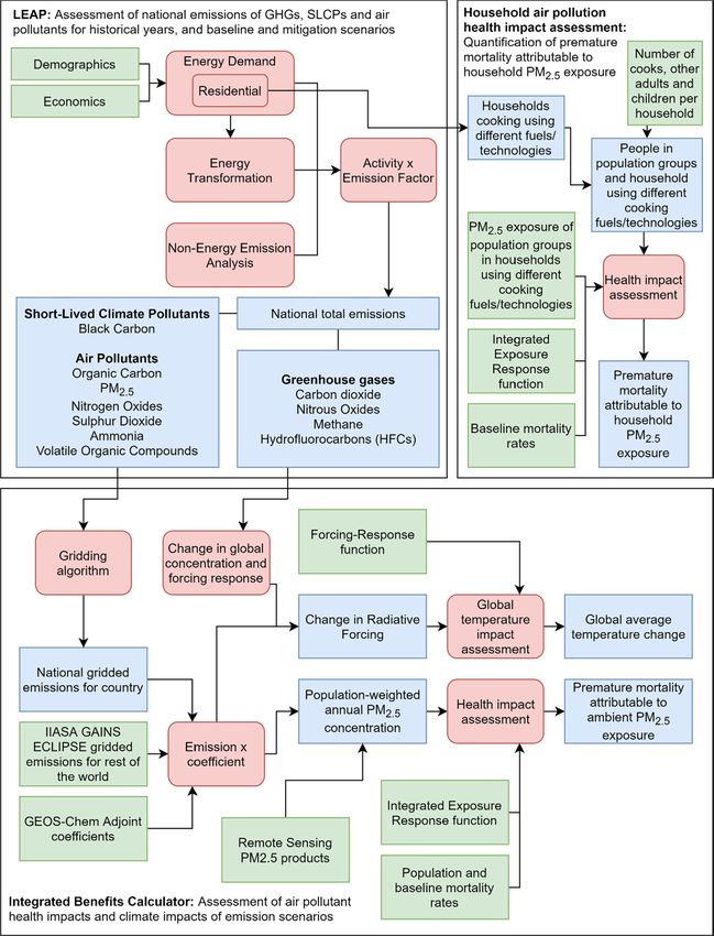
resource intensive and not widely undertaken in LMICs. within LEAP. Results are returned for display using LEAP’s results
This paper describes the development and application of LEAP-IBC. visualization capabilities (charts, tables, maps, energy balances, sankey
The Low Emissions Analysis Platform (LEAP) system, is a scenario- diagrams, etc., an example of which is shown in Fig. 2). The overall
based planning framework for integrated planning of energy policy system makes extensive use of LEAP’s Application Programming Inter
and emissions abatement, developed over the last 30 years at the face (API), a system that allows LEAP to be closely connected to other
Stockholm Environment Institute (Heaps, 2020). LEAP has recently been models and tools based on a programmable interface and a series of
updated to include a new calculation module called IBC, the Integrated additional external scripts that connect LEAP and the IBC calculator. The
Benefits Calculator. IBC is integrated within LEAP, and calculates PM2.5- following sub-sections describe in more detail the approach to devel
attributable health (premature mortality), and climate (global temper oping emission estimates for different scenarios (Section 2.1.1), the
ature change) impacts for different emissions scenarios developed conversion of emissions to ambient PM2.5 concentrations (Section
2
J.C.I. Kuylenstierna et al. Environment International 145 (2020) 106155
2.1.2), and exposure to household air pollution (Section 2.1.3) and the national or sub-national models are supported), time-frame, and the
health (Section 2.1.4) and climate (Section 2.1.5) impact assessment emission sources that are modelled. There are then requirements for
methodologies included in LEAP-IBC. models to be compatible with modelling of air pollution and climate
change impacts using IBC. Firstly, the modelling of PM2.5 concentrations
2.1.1. Emission inventory and scenario modelling described in Section 2.1.2 is available only at the national scale, and
LEAP is flexible with regard to geographic scale (i.e. regional, therefore a national model must be developed. Secondly, the PM2.5
Fig. 1. Schematic of LEAP-IBC framework for estimating emissions for different scenarios and the resultant population-weighted annual average PM2.5 concen
tration, health impacts, and impact on global average temperature change. Key inputs are shown in green, calculations in red, and outputs in blue. (For interpretation
of the references to colour in this figure legend, the reader is referred to the web version of this article.)
3
J.C.I. Kuylenstierna et al. Environment International 145 (2020) 106155
concentrations in the atmosphere are a result of the combination of Bangladesh), the IBC module converts these emissions into national,
emissions of primary PM2.5 from multiple sources, as well as secondary population-weighted annual average ambient PM2.5 concentrations
formation of PM2.5 from gaseous precursors (Heal et al., 2012). The (hereafter abbreviated to PM2.5PW). The PM2.5PW value is used as the
overall impact of a country on global temperature increases depends on estimate of the average exposure of the population of the target country
the balance of emissions of substances that warm the atmosphere (e.g. to PM2.5, for use in the health impact assessment (Section 2.1.3).
GHGs and black carbon) and those that cool the atmosphere (e.g. cooling PM2.5PW is calculated for the target country for each year and for each
aerosols like organic carbon, and secondary inorganic aerosols. There scenario. Ambient PM2.5 concentrations in a country depend on emis
fore, to robustly estimate PM2.5 concentrations, attributable health im sions of PM2.5 and PM2.5-precursors in the target country, and emissions
pacts and impacts on global temperature change, a complete inventory in other countries that are transported into the country. The impact of
of GHG, SLCP, and air pollution emissions from all major source sectors these emissions on PM2.5 in the target country depends on where they
is required. For this reason, a LEAP model used in combination with IBC are emitted, and therefore gridded emission estimates of each pollutant
should quantify total national emissions of GHGs (carbon dioxide, are developed for both national and ‘rest of world’ emissions.
methane, nitrous oxide, hydrofluorocarbons), SLCPs (black carbon, National total emissions of primary PM2.5 (black carbon, organic
methane, HFCs), and other air pollutants (nitrogen oxides, non-methane carbon and other primary PM emissions), and secondary inorganic PM2.5
volatile organic compounds, sulphur dioxide, ammonia, primary par precursors (NOx, SO2 and NH3) derived using LEAP for the target
ticulate matter (PM2.5, PM10, made up of organic carbon, black carbon country are spatially distributed into 2◦ × 2.5◦ grids covering the
and mineral dust), carbon monoxide). Emissions from all major sources country to match the scale of the GEOS-Chem Adjoint model results (see
of these substances must be quantified, including the energy, industrial below). The proportion of national total emissions of each pollutant
processes, waste, and agricultural sectors. A default LEAP model has assigned to the 2◦ × 2.5◦ grids covering the country was based on the
been developed which meets these requirements. It was used to develop spatial distribution of emissions across Bangladesh in an existing grid
the analysis for Bangladesh and is outlined in Section 2.2. While this ded emission dataset, the IIASA GAINS ECLIPSE emissions dataset (Stohl
LEAP model contains a set of methods for estimating emissions of GHGs, et al., 2015). The ECLIPSE estimates emissions of SLCPs and air pollut
SLCPs and air pollutants from all major source sectors, LEAP can ants for historical and future projections in 0.5◦ grids globally. For those
accommodate a range of methods for estimating emissions from energy grids that cover the target country, the ECLIPSE emissions were appor
and non-energy sectors (e.g. higher Tier IPCC or EMEP/EEA methods tioned by population (based on Gridded Population of the World v3
could be used to estimate emissions if data was available (EMEP/EEA, dataset (CIESIN, 2005)). This ensured that the LEAP-derived emissions
2016; IPCC, 2006)), as well as country-specific activity and emission only replace the emissions associated with the target country. Emissions
factors if available. from the rest of the world are represented by the gridded ECLIPSE
emissions outside of the target country, aggregated from the native 0.5◦
2.1.2. Modelling ambient PM2.5 exposure grids to 2◦ × 2.5◦ .
Once national total emissions of GHGs, SLCPs and air pollutants have Next, to translate gridded emissions to PM2.5PW, accounting for
been estimated using LEAP for all major source sectors, for historical transport and chemical processing in the atmosphere, tgidded emissions
years, and future scenarios (e.g. as described in Section 2.2. for are then combined with parameterized output from the adjoint of the
Fig. 2. A screenshot showing health impacts results calculated in IBC being displayed within LEAP’s Graphical User Interface (Sample Results).
4
J.C.I. Kuylenstierna et al. Environment International 145 (2020) 106155
GEOS-Chem global atmospheric chemistry transport model (Bey et al., ∑ PM2.5 2010i pi fi
2001; Henze et al., 2007). The GEOS-Chem Adjoint model output PM 2.5PW 2010 = (2)
pt
quantifies the relationship between emissions of a particular pollutant i
that contributes directly to PM2.5 (BC, OC or other PM), or is a precursor
where pi is the population in each 0.1◦ × 0.1◦ grid in the target country, fi
to PM2.5 (NOx, SO2 and NH3) in any location, and the associated change
is the fraction of the population in each 0.1◦ × 0.1◦ grid that are clas
in PM2.5 in the target country. GEOS-Chem simulates the formation and
sified as being in the target country and pt is the total population in the
fate of pollutants globally at a grid resolution of 2◦ × 2.5◦ , with 47
target country.
vertical levels. Emissions of aerosols and aerosol precursors include both
Gridded (2◦ × 2.5◦ ) PM2.5 concentrations in 2010 from natural
natural (i.e., ocean, volcanic, lightning, soil, biomass burning, biogenic
background emissions, and from natural and anthropogenic PM2.5
and dust) and anthropogenic (transportation, energy, residential, agri
concentrations were calculated from GEOS-Chem and used to calculate
cultural, etc.) sources. The model accounts for the transport and hy
population-weighted annual PM2.5 concentrations for the target country
drophilic aging and removal of primary carbonaceous aerosols (BC and
from natural and total emissions in 2010 (PM2.5PW_GC_nat, and
OC) (Park et al., 2003) along with heterogeneous surface chemistry
PM2.5PW_GC_tot, respectively). PM2.5 concentrations are calculated at 35%
(Evans and Jacob, 2005), aerosol feedbacks on photolysis rates (Martin
RH and standard temperature and pressure; satellite-derived estimates
et al., 2003), and partitioning of secondary inorganic aerosols (sulfate,
of the organic matter to OC ratio from Philip et al. (2014) are applied
nitrate, and ammonium) (Park, 2004). The adjoint of the GEOS-Chem
seasonally. The anthropogenic fraction (PM2.5PW_GC_anth) was calculated
model calculates the sensitivity of a particular model response metric
by subtraction (Equation (3)). The natural concentration of PM2.5PW_2010
(in this case population-weighted annual average surface PM2.5 con
(PM2.5PW_nat) was then calculated with Equation (4), and this was
centration across the target country) with respect to an emission
assumed to be constant for all future years and scenarios. The anthro
perturbation in any of the global model 2◦ × 2.5◦ grid cells (Henze et al.,
pogenic component of PM2.5PW_2010 (PM2.5PW_2010_anth) was then esti
2007), accounting for all of the mechanisms related to aerosol formation
mated through subtraction (Equation (5)).
and fate. These sensitivities are output from the GEOS-Chem adjoint as
gridded ‘coefficients’, which are then multiplied by emission estimates PM 2.5PW GC anth = PM 2.5PW GC tot − PM 2.5PW GC nat (3)
in IBC to estimate the change in PM2.5PW for each year and emission
scenario. For more details, see previous applications of GEOS-Chem PM 2.5PW nat = PM 2.5PW 2010 *
PM 2.5PW GC nat
(4)
adjoint coefficients for estimating responses to spatially explicit emis PM 2.5PW GC tot
sions changes (e.g. Henze et al., 2012; Lacey and Henze, 2015; Lacey
PM 2.5PW = PM 2.5PW − PM 2.5PW (5)
et al., 2017; Lapina et al., 2015; Paulot et al., 2013). 2010 anth 2010 nat
Adjoint coefficients were produced for each pollutant that contrib The PM2.5PW_2010_anth component was further disaggregated into
utes to PM2.5PW concentrations, namely, BC, OC, NOx, SO2, NH3 and contributions from emissions of each primary PM2.5 (black carbon,
other PM (in this case, predominantly mineral dust), reflecting their organic carbon, other primary PM) or PM2.5 precursor pollutant (ni
different reactivity and formation pathways in the atmosphere. The trogen oxides, sulphur dioxide, ammonia), and the contribution from
adjoint coefficients are applied by multiplying, in each grid and for each emissions in the target country, and from emissions from grid squares
pollutant, the coefficient by emissions, and summing across all grids to outside of the country (rest of the world emissions). For each pollutant,
estimate the change in PM2.5PW for a particular year for a particular for the target country and rest of the world emissions separately, the
scenario. contribution to PM2.5PW_2010_anth was calculated by i) summing, across
A limitation of the application of the adjoint coefficients is that they all grids globally, the product of the adjoint coefficients parameterised
provide a linear representation of the response of PM2.5PW to emissions for that pollutant and the pollutant emissions in the grids covering the
perturbations, which leads to uncertainty when emission perturbations target country or rest of the world emissions, and ii) scaling these values
are large (considered to be approximately > 50% for NOx, SO2, and NH3 so that the sum for all pollutants equalled PM2.5PW_2010_anth.
impacts on PM2.5 (Henze et al., 2012; Lee et al., 2015)). Another limi The impact of changes in emissions for future scenarios on PM2.5PW
tation of applying a model with a resolution of 2◦ × 2.5◦ is uncertainty in are calculated by multiplying the adjoint coefficients for each grid, for
estimated PM2.5PW concentrations owing to strong gradients in popu each PM2.5 and PM2.5-precursor pollutant, by the difference in emissions
lation that may be up to 30–50% (Punger and West, 2013). Additionally, between 2010 and the future year in a particular scenario. The change in
baseline PM2.5 values estimated in the present day by GEOS-Chem may emission in the grids covering the rest of the world, in the baseline
have biases. To overcome these limitations, the gridded GEOS-Chem scenario, is estimated from the ECLIPSE current legislation scenario
values of PM2.5 (PM2.5_GC) were downscaled at the 0.1◦ × 0.1◦ resolu (Stohl et al., 2015). The change in emissions in the grids covering the
tion using surface PM2.5 concentrations from van Donkelaar et al. target country are calculated by subtracting the emissions of each
(2016). These are derived from a combination of satellite and modelled pollutant in the future year for a given scenario (baseline or mitigation)
PM2.5 data, calibrated to a global network on ground-based PM2.5 from the values in 2010. The sum of the coefficient × change in emission
measurement. The downscaling occurs through multiplication of the for each pollutant for each grid is then scaled by the ratio of
average ratio of the PM2.5 from van Donkelaar et al. (2016) at the 0.1◦ × PM2.5PW_2010_anth to PM2.5PW_GC_anth to provide the estimate of the change
0.1◦ resolution to the van Donkelaar et al. (2016) values averaged to the in PM2.5PW in the future year due to changes in emissions of each
2◦ × 2.5◦ resolution, PM2.5_vanD2016 / PM2.5_vanD2016_2x25. Additionally, pollutant for a particular scenario that is consistent with the PM2.5PW
for 2010 estimates, an additional bias correction factor is applied, which value set to the van Donkelaar et al. (2016)-derived value in 2010.
is the ratio of van Donkelaar et al. (2016) estimates to the GEOS-Chem
estimates, both at the 2◦ × 2.5◦ resolution, PM2.5_vanD2016_2x25 / PM2.5_GC, 2.1.3. Household PM2.5 exposure
which essentially reduces to using the 0.1◦ × 0.1◦ values from van In addition to modelling ambient PM2.5 exposure and health impacts
Donkelaar et al. (2016). National average population weighted con in IBC, the latest versions of LEAP also include methods for estimating
centrations (PM2.5PW) are then calculated from these, which in 2010 was the health impacts associated with exposure to PM2.5 pollution from
calculated to be 52.1 µg m− 3 in Bangladesh (Equation (1)). cooking in households, which is associated with substantial health
PM 2.5 vanD2016 PM 2.5 vanD2016 burdens (Stanaway et al., 2018). The methods implemented in LEAP for
GC * * estimating cooking-related impacts are based upon a set of methods
2x2.5
PM 2.5 2010 = PM 2.5
PM 2.5 vanD2016 2x2.5 PM 2.5 GC
developed and implemented in the Household Air Pollution Intervention
= PM 2.5 (1)
VanD2016
Tool (HAPIT III) (Pillarisetti et al., 2016). These methods are consistent
5
J.C.I. Kuylenstierna et al. Environment International 145 (2020) 106155
with those used to quantify global burdens of disease attributable to Equations (6) and (7) to estimate the number of premature deaths
household PM2.5 exposure (WHO, 2018). The methods used in HAPIT III attributable to ambient PM2.5 exposure for each year in the analysis, and
were originally intended to be applied in small-scale, static assessments for each scenario, i.e. historical years, and future years for baseline and
of the potential benefits of interventions at the village-scale to promote mitigation scenarios. Personal PM2.5 exposure from household sources
clean cooking. In LEAP, we have adapted those methods to make them estimated for each population group (primary cook, other adults and
suitable for use at the national-scale, and have made them dynamic and children under 5 years) living in households cooking with different
scenario-based so that they can show the comparative benefits of tran fuels/technologies is combined with Equation (6) and (7) to estimate the
sitioning societies away from a reliance on traditional cooking and to number of premature deaths attributable to household air pollution for
ward cleaner cooking technologies. each year/scenario.
Modelling of indoor air pollution in LEAP accounts for six separate Household and ambient air pollution and two overlapping risk fac
groups of households members: male and female primary cooks, other tors for premature mortality. For example, residents in households
male and female adults and male and female children (under five years cooking using solid biomass, exposed to high levels of household air
old). The number of primary cooks, other adults and children living in pollution may also be exposed to high levels of ambient air pollution.
households cooking using different types of fuels and technologies is This is particularly the case in countries such as Bangladesh where i) a
then calculated by multiplying the number of households cooking using high proportion of the population cooks using solid fuels, and ii) outdoor
a particular fuel/technology by the fraction of the average household PM2.5 concentrations are many times higher than the WHO ambient air
size that are primary cooks, other adults and children. For each cooking quality guideline for the protection of human health (i.e. an annual
fuel/technology combination, the 24-hour personal exposure of the average of 10 µg/m3). Due to uncertainties in the degree of overlap
primary cook is specified for each cooking technology and relative ex between exposures to household and ambient air pollution in
posures are defined for other groups of household members. This pro Bangladesh, health impacts from both sources of exposure are reported
vides the number of people in each population group and their personal separately in this study. Within the LEAP-IBC platform, health impacts
PM2.5 exposure which is used as input to the health impact assessment from household and ambient PM2.5 exposure can be combined to esti
described in section 2.1.4. mate the overall air pollution health burden using the approach outlined
Currently, the methodology accounts only for cooking technologies. in Ezzati et al. (2003) for combining multiple independent risk factors.
Exposure to other sources of indoor PM2.5, such as kerosene use for
lighting or smoking are not included. The specific application of this 2.1.5. Climate impact assessment
method to estimate household air pollution health impacts in LEAP calculates Global Warming Potential (GWP) using standard
Bangladesh is described in Section 2.2. factors taken from IPCC assessment reports. To allow LEAP to be useful
in national GHG mitigation assessments, it supports a range of different
2.1.4. PM2.5 health impact assessment GWP factors reflecting the revisions made in successive IPCC assessment
In the LEAP-IBC framework, the health endpoint for which the reports (Myhre et al., 2013). In addition, in order to give more accurate
impact of ambient and household PM2.5 exposure is estimated is pre assessments of likely year-on-year global warming, LEAP-IBC can also be
mature mortality. Premature mortality attributable to PM2.5 exposure is used to estimate the contribution to global temperature change of the
estimated for children (less than 5 years) and adults (>30 years) in − 5- national-scale emissions calculated within LEAP.
year age groups (30–34, 35-39…75-79, >80 years) from 5 disease cat To allow the impacts of different future emissions on climate change
egories (children: acute lower respiratory infection; adults: chronic to be evaluated, transient changes in global surface temperature, in
obstructive pulmonary disease, ischemic heart disease, cerebrovascular annual time steps, are calculated accounting for the climate effects of
disease and lung cancer). The PM2.5PW estimate of exposure to ambient both short-lived climate forcers (SLCFs) and greenhouse gases. In this
PM2.5 concentrations, and the personal PM2.5 exposure for different applications SLCFs include short-lived climate pollutants (SLCPs), i.e.
population groups to household PM2.5, are combined separately with black carbon, tropospheric ozone and methane, which are relatively
‘integrated exposure response’ (IER) functions that have previously been short-lived in the atmosphere and have a warming impacts, but also
extensively used for quantifying air pollution health burdens (Burnett short-lived species that have a cooling impact, i.e. organic carbon and
et al., 2014; Cohen et al., 2017). The IER functions (Equation (6)) secondary inorganic aerosol. Methane is also a greenhouse gas, and
quantify the relative risk (RR) for mortality from specific diseases for therefore the methods to quantify the impact of methane on global
PM2.5 exposures up to very high levels (up to 10,000 µg m− 3), by inte temperatures is described alongside other greenhouse gases, such as
grating RRs derived from epidemiological studies between cause- carbon dioxide.
specific mortality and PM2.5 exposure from ambient air pollution, The methodology included in LEAP-IBC to achieve the transient
household air pollution, second hand smoke, and active smoking. climate calculations has been described previously in Lacey and Henze
δ
(2015), and Lacey et al. (2017). For all climate forcers, the change in
RRIER = 1 + α(1 − e− γ(z− zcf )
) (6) radiative forcing of those emissions are estimated in 4 latitudinal bands
(arctic, northern mid-latitudes, tropics, and southern hemisphere extra-
where zcf is the PM2.5 low concentration cut-off, z is the PM2.5 concen tropics), following the framework developed in Shindell and Faluvegi
tration that a population is exposed to, and α, δ, and γ are IER-specific (2009) and Shindell (2012). The transient surface temperature change,
parameters (Burnett et al., 2014; Cohen et al., 2017). The RR derived relative to the base year of the analysis can then be estimated without
from the IER function for a particular disease and age group, is then used additional global climate model simulations by using the absolute
in combination with the baseline mortality rate for that disease for the regional temperature potentials forcing-response relationships (Shindell
population in the target country, and the exposed population in the age and Faluvegi, 2009; Shindell, 2012). The use of this parameterization
category in the target country to estimate the number of premature has been evaluated through comparisons to a number of fully coupled
deaths attributable to ambient PM2.5 exposure from the particular dis chemistry-climate models for both the global temperature response
ease in that age group (Equation (7)). (Stohl et al., 2015) and the regional temperature responses (Sand et al.,
(
RRIER − 1
) 2013). The methods for both SLCPs and long-lived GHGs are outlined in
ΔMort = y0 Pop (7) the following sections.
RRIER
Here y0 is the baseline mortality rate for each disease category, and 2.1.5.1. Short-lived climate forcers. In order to calculate the radiative
Pop is the exposed population for each child or adult age category. The forcing from aerosols, the GEOS-Chem model is combined with a
ambient PM2.5PW estimated as described in Section 2.1.2 is used with
6
J.C.I. Kuylenstierna et al. Environment International 145 (2020) 106155
radiative transfer model (RTM), LIDORT (Spurr et al., 2001). Aerosol ∫ tf ∑
4
species from GEOS-Chem are assigned species-specific optical properties 1 tf − t tf − t
ΔTregion = Fi δi,r x x(2.507xe 4.1 + 0.027xe 219 ) (9)
(refractive index and size distribution) and the assumption of a fully t0 i=1
18.498
external mixture of aerosols is used with Mie theory to calculate gridded
aerosol optical depths, phase functions, and single scattering albedo that where the summation of regional radiative forcings is the weighted
are input to the RTM (Henze et al., 2012). Radiative effects at the top-of- radiative forcing from short-lived species calculated using the RTP co
the-atmosphere (TOA) are calculated over the wavelengths of incoming efficients (Lacey and Henze, 2015; Shindell and Faluvegi, 2009), and t is
solar radiation. In order to calculate radiative forcing, the radiative flux the year of interest between t0 (baseline) and tf (endpoint). For short-
from a pre-industrial case (1850) is subtracted from the present-day TOA lived species the change in radiative forcing is considered to be instan
flux calculated using the GEOS-Chem modelled concentrations of aero taneous and felt within the year of emission. The first exponential term
sols and other trace constituents in the atmosphere (Henze et al., 2012; in the integral relates to the response of the surface and shallow seas,
Lacey and Henze, 2015). LIDORT calculates the Jacobian matrix of in and the second exponential term relates to the thermal inertia of the
puts (optical properties) with respect to outputs (gridded radiative flux); deep ocean. Finally, for each pollutant, for each year, for each scenario,
these derivatives are used as inputs to the GEOS-Chem adjoint model, a global area-weighted mean temperature change is then calculated
which is able to propagate these sensitivities of radiative forcing with from the latitudinal band temperature changes.
respect to changes in optical properties back to sensitivities with respect
to gridded global emissions of individual aerosol and aerosol precursor 2.1.5.2. Greenhouse gases. For GHGs like CO2 and CH4, the change in RF
species. Ozone radiative forcing is calculated following Bowman and resulting from their emission in a particular year is not confined to the
Henze (2012), which is summarized as follows. Remote sensing obser year in which they were emitted, but as a function of time from the year
vations of the sensitivity of outgoing longwave radiation to the 3D dis of emission due to their longer atmospheric lifetimes. Hence for an
tribution of tropospheric O3 is quantified using the Instantaneous emission of CO2 and CH4, it is assumed that their emission from any
Radiative Kernels (IRK) measured by the Thermal Emission Spectrom location becomes globally mixed, and therefore the first step in esti
eter (TES) aboard the Aura satellite (Worden et al., 2011; 2008). The mating temperature change from CO2 and CH4 is to estimate the change
GEOS-Chem adjoint model is used to apportion this radiative effect from in global CO2 and CH4 concentrations due to shifts in emissions in the
all tropospheric O3 to its contributions from anthropogenic emissions to target country. Therefore, in the year of emissions, a 1 Gt change in
derive an O3 radiative forcing per unit emission of NOx, NMVOCs, and emissions of CO2 and CH4 were associated with a 0.128 ppm and 0.278
CO. ppm change in global CO2 and CH4 concentrations, respectively. The
The change in radiative forcing (RF) in the four latitudinal bands was decay in CO2 and CH4 concentrations in the years following emission
calculated for emissions that contribute to aerosol formation (i.e. BC, were then represented by impulse response functions (IRF), shown in
OC, NH3, NOx, SO2), and ozone precursors (i.e. NOx, CO, VOCs). Once Equations (10) and (11), respectively.
formed, the lifetimes of aerosols and ozone are short enough that the ( ) ( ) ( )
pollutants are not globally mixed, and therefore the location of emis − y+b − y+b − y+b
(10)
394.4 36.5 4.304
sions of these pollutants determines the effect of these emissions on IRF CO2 = 0.217 + 0.224*e + 0.282*e + 0.276*e
radiative forcing in each latitudinal band. Hence, for each pollutant that ( )
contribute to aerosol and ozone formation, four sets of linearised co − y+b
(11)
12.4
efficients were produced from the GEOS-Chem adjoint model that IRF CH4 = e
quantify the sensitivity of radiative forcing in each latitudinal band to
emissions of a pollutant in 2◦ × 2.5◦ grids covering the globe. The where y is the year of interest after emission and b is the year of emis
calculation of these adjoint coefficient for latitudinal band radiative sion. The parameters of IRFCO2 were derived from model calculations in
forcing are described in detailed in Lacey and Henze (2015). These co Joos et al. (2013). The IRFs are used to calculate the time-dependent
efficients also include scaling factors to incorporate species-specific response of concentrations in year t owing to emissions changes from
biases and uncertainty ranges based on multi-model studies of aerosol years b to y.
radiative forcing (Boucher et al., 2013; Myhre et al., 2013). For each [C]y = β*sum(σ(y)*IRF(y) ) + [C]b (12)
year and each scenario, the emissions of these pollutants in the target
country, derived in LEAP, are multiplied by the coefficients to determine where β is the unit conversion from global annual emissions (in giga
the time-dependent change in radiative forcing in each latitudinal band tonnes) to parts per million for CO2 and parts per billion for CH4 and
(Flat) due to emissions in the target country (Equation (8)). N2O, σ is the change in emissions in gigatonnes in year y, and Cb is the
Flat = Eλα (8) global background concentration in the base year b. Following the
calculation of CO2 and CH4 concentration changes, the change in global
where E are the time and species dependent emissions, λ are the adjoint radiative forcing in each year due to these concentration changes are
sensitivities, and ⍺ are the radiative forcing scaling factors. Radiative calculated. For CO2, the change in global RF was calculated using
forcing in individual latitudinal bands then results in a localized tem Equation (13), and for CH4, Equation (14) was used, and were derived in
perature response in each of the four latitudinal bands (i.e. a change in Aamas et al. (2013).
radiative forcing in the arctic produces a temperature response in the
[CO2 ]y
northern mid-latitude, tropics, and southern hemisphere extratropics RFCO2 = 5.35*ln( ) (13)
[CO2 ]ref
regions, as well as in the arctic itself) as shown in Shindell and Faluvegi
(2009). These regional temperature potential coefficients quantify the
sensitivity of the temperature response in one region to a radiative RFCH4 = 0.036*(([CH4 ]y 0.5 − [CH4 ]ref 0.5 ) − 0.47*ln(1
( )0.75
forcing in another region, relative to the global mean temperature
+ 2.01x10− 5 * [CH 4 ]y *[N2 O]ref
sensitivity. Hence for a given year after emission, the net change in
( )1.52
radiative from all regions was weighted using absolute regional tem + 5.31x10− 15 *[CH 4 ]y * [CH 4 ]y *[N2 O]ref ) + 0.47*ln(1
perature potentials (δ) and translated into the temperature change using ( )0.75
multi-model mean results for the integrated transient climate sensitivity + 2.01x10− 5 * [CH 4 ]ref *[N2 O]ref
(Geoffroy et al., 2013) (Equation (9)). ( )1.52
+ 5.31x10− 15 *[CH 4 ]ref * [CH 4 ]ref *[N2 O]ref ) (14)
7
J.C.I. Kuylenstierna et al. Environment International 145 (2020) 106155
where [CO2]y, and [CH4]y, represents the global CO2 and CH4 concen and projections were made to 2030 and 2040.
trations in the year of interest for a particular scenario, accounting for The methods and data used to develop the LEAP model for
the change in concentration due to emissions in the target country in all Bangladesh are outlined comprehensively in Department of Environ
years between the base year and the year of interest. The variables ment (2018). Table 1 summarises the key data used to estimate emis
[CO2]ref, [CH4]ref, and [N2O]ref represent global average concentrations sions from all major energy and non-energy source sectors, including the
of each pollutant in a reference year, and were set at 378 ppm, 1726 ppb, methods used for projecting emissions into the future for a business as
and 318 ppb, respectively, corresponding to their values in 2010, the usual scenario. The LEAP model developed was the first emission in
base year of the analysis (Lacey et al., 2017). From this global radiative ventory and scenario assessment for Bangladesh that estimated emis
forcing, the temperature change resulting from CO2 and CH4 emissions sions of all GHGs, SLCPs and air pollutants in a single, consistent
in Bangladesh were calculated in each year using Equation (9). In these analysis. However, Bangladesh has developed dedicated GHG emission
cases the sensitivity of the temperature response in each region uses inventories and projections as part of the UNFCCC climate change
global radiative forcing with the global mean temperature sensitivity, reporting processes (i.e. within National Communication and Biennial
also derived in Shindell (2012). Update Reports). Therefore, to ensure that the emission estimates of
SLCPs and air pollutants were consistent with official GHG inventories
and mitigation assessments, data and projection assumptions in the
2.1.5.3. Additional climate feedbacks. Changes in the emissions of some
LEAP model were aligned with those used in the GHG mitigation
pollutants also change atmospheric composition in a way that feeds back
assessment conducted for Bangladesh’s Third National Communication
on other radiatively active components; such feedbacks need to be taken
(Ministry of Environment Forest and Climate Change Bangladesh,
into account when estimating the overall climate impact of a particular
2018). For each source sector, emissions were calculated by multiplying
change in emission magnitude. Therefore, the impact of changes in NOx,
an activity variable by pollutant specific emission factors. The specific
CO, and VOC emissions on CH4 concentrations and associated climate
activity variables, as well as the source of emission factors are described
impacts are accounted for. Increases in NOx emissions reduce CH4,
in Table 1 for each of the source sectors included in the analysis.
because of the increased CH4 sink through O3 formation. Increases in CO
For the majority of energy demand sectors, the activity variable was
and VOC emissions increase CH4 RF due to the lower availability of
the total fuel consumption for that sector extracted from International
oxidants to react with CH4. The response of CH4 RF to changes in VOC
Energy Agency (IEA) energy statistics (International Energy Agency,
and CO emissions was taken from a multi-model experiment assessing
2015). For these sectors, emission factors for the GHGs were Tier 1
the RF responses of decreases in pollutant emissions described in Fry
factors from the Intergovernmental Panel on Climate Change (IPCC)
et al. (2012). Between the different regions assessed, there was a fairly
Guidelines for Greenhouse Gas Inventories (IPCC, 2006), and for other
consistent response to CH4 RF for a change in CO and VOC emissions,
species were Tier 1 and Tier 2 factors from the EMEP/EEA (2016)
which was on average 66% and 127% of the change in O3 RF due to the
Emission Inventory Guidebook (summarised in detail in Vallack et al.
same change in VOC and CO emissions, respectively. Hence, to account
(2020), and available at https://leap.sei.org/default.asp?action = IBC.
for the change in CH4 RF due to changes in these emissions, the esti
More detailed methods were used to estimate emissions from brick kilns,
mated change in O3 RF due to VOC and CO emissions, described above
rice parboiling and road transport. Brick kiln emissions were estimated
was scaled by these factors.
as the product of the total number of bricks produced per year, dis
The estimated change in CH4 RF due to a change in NOx emissions
aggregated between ‘traditional’ and ‘improved’ kilns, the energy in
differed by region. We therefore developed regional factors (unit mW
tensity per brick produced for each type of brick kiln, and kiln-specific
m− 2 Tg NOx emission-1) that quantify the change in CH4 RF for a change
emission factors for each pollutant. For rice parboiling, emissions were
in NOx emissions based on the work of Naik et al. (2005). The temper
calculated as the product of the total rice parboiled, the energy con
ature responses to these additional changes in RF were calculated using
sumption per tonne of rice parboiled, and emission factors for traditional
Equation (9) for each latitudinal band, then aggregated to an area-
and improved rice kilns. For the road transport sector, the number of
weighted global mean.
vehicle-km travelled by passenger cars, light duty vehicles, heavy duty
Lastly, we also consider the RF impacts of the emissions of BC aerosol
vehicles, motorcycles, three wheelers and urban buses were estimated,
by altering the albedo of snow and ice upon which BC may deposit, as
and disaggregated between vehicles using different fuels (gasoline,
described in Lacey and Henze (2015). The total global snow/ice albedo
diesel, CNG etc.), and meeting different vehicle emission (Euro) stan
effect of − 0.15 W/m2 is apportioned across all BC sources using the
dards. Tier 2 default emission factors (g pollutant per km travelled) from
results of an additional adjoint model calculation. This calculation
the EMEP/EEA (2016) Emission Inventory Guidebook were used to es
considered as a model response the deposition of BC onto snow and ice.
timate emissions of all pollutants except CO2, SO2 and CH4, where
The results then relate the BC emissions in any grid cell to the amount of
emission factors were used based on total fuel consumed. For all energy
BC deposited on snow and ice. The impact of this radiative effect on
sectors (including transport), the uncontrolled fuel combustion emission
transient temperature estimates follows the treatment of other short-
factors for SO2 were derived from the sulphur (S) content of the fuel
term RF using Eq. (9).
assuming all the S is ultimately oxidised to SO2, after accounting for S
retention in ash for solids fuels.
2.2. Application to air pollution and climate change mitigation in Emissions from the energy transformation sectors were calculated
Bangladesh based on the demand for fuels for each of the energy demand sectors. For
electricity generation, the share of electricity generated using different
The application of the LEAP-IBC modelling framework shown in technologies and fuels was based on IEA energy balance statistics (In
Fig. 1, and described in Section 2.1 aimed to evaluate the effect on air ternational Energy Agency, 2015). Transmission and distribution losses
quality and climate change of two key strategies, Bangladesh’s NDC in electricity generation were extracted from World Bank statistics
(Ministry of Environment and Forests, 2015), and National Action Plan (databank.worldbank.org). Finally, the emissions from other sectors
to reduce SLCPs (Bangladesh Department of Environment, 2018). The were estimated using the activity data for each source described in
first step was to develop a LEAP model application that estimated na Table 1. The calculation of GHG emissions for the majority of the non-
tional total emissions of GHGs, SLCPs and air pollutants from all major energy sectors followed the Tier 1 methodologies outlined in the Inter
source sectors, in alignment with the results of National Greenhouse Gas governmental Panel on Climate Change (IPCC) Guidelines for Green
inventory, and meeting the requirements for compatibility with the IBC house Gas Inventories (IPCC, 2006) whereas estimates of emissions from
module for assessing air pollution and health impacts (described in all other pollutants followed the Tier 1 methods and emission factors
Section 2.1.1). The base year for the Bangladesh LEAP model was 2010, given in the EMEP/EEA (2016) Emission Inventory Guidebook.
8
J.C.I. Kuylenstierna et al. Environment International 145 (2020) 106155
Table 1 Table 1 (continued )
Summary of emission source sectors included in the Bangladesh emission in Source Sector IPCC Activity Data and source Baseline scenario
ventory, source of activity data and assumptions about development of baseline Source projection method
emission scenarios for analysis described in Department of Environment (2018). Code
For all sources, emission factors were taken from IPCC (2006) for GHGs, and
Electricity Electricity matrix: IEA Electricity generation
EMEP/EEA (2016) and other scientific literature for black carbon and other air
Generation energy balance for increases according to
pollutants, available at: https://leap.sei.org/default.asp?action=IBC. Bangladesh increases in electricity
Source Sector IPCC Activity Data and source Baseline scenario demand. Changes in
Source projection method electricity matrix based
Code on projected changes
made in Bangladesh’s
Residential 1A4b Number of households ( Growth in energy Third National
UN DESA, 2019, 2018) consumption based on Communication
projection in Industrial 2A-2D Mineral Production: US Growth in line with
Total fuel consumption: Bangladesh Third Processes Geological Survey increases in industrial
IEA energy balance for National Mineral Yearbook energy consumption
Bangladesh Communication
Commercial 1A4a Total fuel consumption: Growth in energy Chemical and food and
and Public IEA energy balance for consumption based on drink production: FAO
Services Bangladesh projection in Stat
Bangladesh Third Agriculture 3A, 3C Animal Numbers: Agricultural activity
National Department of projected based on
Communication Livestock, http://dls. historical trends
Transport 1A3 Road Transport: Growth in energy portal.gov.bd (assuming
Total number of vehicles consumption based on 60% cattle to be dairy
in each category: projection in cattle)
passenger cars, light Bangladesh Third
commercial vehicles, National Fertiliser consumption:
heavy duty vehicles, Communication FAO Stat
motorcycles, buses
(Bangladesh Road Annual Harvested Area,
Transport Authority, Cultivation period:
www.brta.gov.bd); Fuel Third National
used and distance Communication
travelled (Wadud and
Khan, 2013) Annual Crop
Production: FAO Stat
Rail; Aviation; Shipping: Fraction burnt in the
Total Fuel Consumption: field (Haider, 2013)
IEA energy balance for Waste 4A, 4B, Waste sent to landfill: Waste generation
Bangladesh 4D IPCC Tier 1 default projected in line with
Industry 1A2 All industry except brick Growth in energy values population increases
kilns: Total fuel consumption based on
consumption: IEA projection in Waste openly burned (
energy balance for Bangladesh Third Wiedinmyer et al.,
Bangladesh National 2014)
Communication
Brick Production:
Annual brick production
The assumptions used to project activity in each sector into the future
Kiln composition
Energy intensity for the baseline scenario are summarised in Table 1. For most energy
(World Bank, 2011) demand source sectors the baseline projection of energy consumption to
Agriculture, 1A4c Total fuel consumption: Growth in energy 2040 was assumed to follow the same trajectory as described in Ban
Forestry and IEA energy balance for consumption based on gladesh’s 3rd National Communication submitted to the UNFCCC
Fishing Bangladesh projection in
Bangladesh Third
(Ministry of Environment Forest and Climate Change Bangladesh,
National 2018). The aim of this work was to evaluate the emission reduction
Communication potential, and impact reductions that could result from implementation
Rice Parboiling N/A Tonnes of rice parboiled Growth in tonnes of rice of the NDC and National SLCP Plan measures in Bangladesh. Therefore,
Energy intensity for parboiled assumed to
the selection of the official baseline projections from Bangladesh’s 3rd
traditional and grow with rice
improved methods production rate National Communication were chosen so that the emission reduction
(GIZ, 2016) potentials estimated in this work were being assessed relative to a
Other Energy 1A5 Total fuel consumption: Growth in energy baseline that was as consistent as possible with previous national ana
Consumption IEA energy balance for consumption based on lyses. Changes in electricity generation were based on changes in de
Bangladesh projection in
Bangladesh Third
mand for those fuels, assuming the electricity matrix remained the same
National as in the base year. The assumptions for the non-energy sector are also
Communication described in Table 1.
Energy 1A1b Total fuel consumption: Growth in energy Mitigation scenarios were developed that represented the imple
Industry IEA energy balance for consumption based on
mentation of individual policies and measures contained within Ban
Own Use Bangladesh projection in
Bangladesh Third gladesh’s NDC and National SLCP Plan (Bangladesh Department of
Oil and Gas genset use: National Environment, 2018; Ministry of Environment and Forests, 2015). The
World Bank Diesel Communication mitigation measures modelled from the NDC, and National SLCP Plan,
Generator Study including targets and timelines, are described in Table 2. The individual
1A1a
mitigation measures were then aggregated to create scenarios that
9You can also read