Impacts of enhanced weathering on biomass production for negative emission technologies and soil hydrology
←
→
Page content transcription
If your browser does not render page correctly, please read the page content below
Biogeosciences, 17, 2107–2133, 2020
https://doi.org/10.5194/bg-17-2107-2020
© Author(s) 2020. This work is distributed under
the Creative Commons Attribution 4.0 License.

Impacts of enhanced weathering on biomass production for negative
emission technologies and soil hydrology
Wagner de Oliveira Garcia1 , Thorben Amann1 , Jens Hartmann1 , Kristine Karstens2 , Alexander Popp2 ,
Lena R. Boysen3 , Pete Smith4 , and Daniel Goll5,6
1 Institute of Geology, Center for Earth System Research and Sustainability, University of Hamburg, Hamburg, Germany
2 Potsdam   Institute for Climate Impact Research (PIK), Potsdam, Germany
3 Land in the Earth System (LES), Max Planck Institute for Meteorology, Hamburg, Germany
4 Institute of Biological and Environmental Sciences, School of Biological Sciences, University of Aberdeen, Aberdeen, UK
5 Laboratoire des Sciences du Climat et de l’Environnement, CEA, CNRS, UVSQ, 91190 Gif-sur-Yvette, France
6 Institute of Geography, University of Augsburg, Augsburg, Germany

Correspondence: Wagner de Oliveira Garcia (wagner.o.garcia@gmail.com)

Received: 24 September 2019 – Discussion started: 9 October 2019
Revised: 21 February 2020 – Accepted: 10 March 2020 – Published: 17 April 2020

Abstract. Limiting global mean temperature changes to well     (∼ 0.2–∼ 27 Gt C) for the specified scenarios (excluding ad-
below 2 ◦ C likely requires a rapid and large-scale deploy-    ditional carbon sequestration via alkalinity production). For
ment of negative emission technologies (NETs). Assess-         BG, 8 kg basalt m−2 a−1 might, on average, replenish the ex-
ments so far have shown a high potential of biomass-based      ported potassium (K) and P by harvest. Using pedotransfer
terrestrial NETs, but only a few assessments have included     functions, we show that the impacts of basalt powder applica-
effects of the commonly found nutrient-deficient soils on      tion on soil hydraulic conductivity and plant-available water,
biomass production. Here, we investigate the deployment        to close predicted P gaps, would depend on basalt and soil
of enhanced weathering (EW) to supply nutrients to areas       texture, but in general the impacts are marginal. We show
of afforestation–reforestation and naturally growing forests   that EW could potentially close the projected P gaps of an
(AR) and bioenergy grasses (BG) that are deficient in phos-    AR scenario and nutrients exported by BG harvest, which
phorus (P), besides the impacts on soil hydrology. Using       would decrease or replace the use of industrial fertilizers. Be-
stoichiometric ratios and biomass estimates from two estab-    sides that, EW ameliorates the soil’s capacity to retain nutri-
lished vegetation models, we calculated the nutrient demand    ents and soil pH and replenish soil nutrient pools. Lastly, EW
of AR and BG. Insufficient geogenic P supply limits C stor-    application could improve plant-available-water capacity de-
age in biomass. For a mean P demand by AR and a low-           pending on deployed amounts of rock powder – adding a new
geogenic-P-supply scenario, AR would sequester 119 Gt C        dimension to the coupling of land-based biomass NETs with
in biomass; for a high-geogenic-P-supply and low-AR-P-         EW.
demand scenario, 187 Gt C would be sequestered in biomass;
and for a low geogenic P supply and high AR P demand,
only 92 Gt C would be accumulated by biomass. An average
amount of ∼ 150 Gt basalt powder applied for EW would be       1   Introduction
needed to close global P gaps and completely sequester pro-
jected amounts of 190 Gt C during the years 2006–2099 for      To limit temperature increase due to climate change to well
the mean AR P demand scenario (2–362 Gt basalt powder for      below 2 ◦ C compared to preindustrial levels by the end of
the low-AR-P-demand and for the high-AR-P-demand sce-          the century, research efforts on negative emission technolo-
narios would be necessary, respectively). The average poten-   gies (NETs; i.e., ways to actively remove CO2 from the
tial of carbon sequestration by EW until 2099 is ∼ 12 Gt C     atmosphere) intensify. Terrestrial NETs encompass bioen-
                                                               ergy with carbon capture and storage (BECCS); afforesta-

Published by Copernicus Publications on behalf of the European Geosciences Union.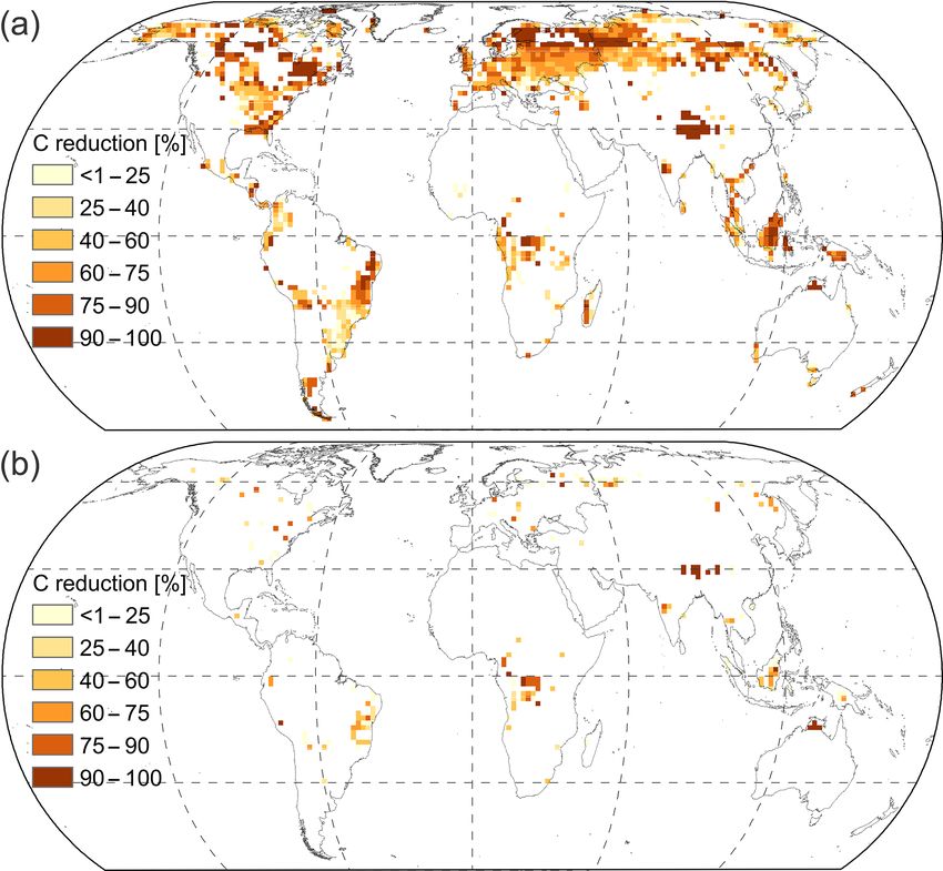
2108                                                               W. de Oliveira Garcia et al.: Impacts of enhanced weathering

tion, reforestation and naturally growing forests (AR); en-            2008; Landeweert et al., 2001; Waldbauer and Chamberlain,
hanced weathering (EW); biochar; restoration of wetlands;              2005; Singh and Schulze, 2015) and controls atmospheric
and soil carbon sequestration. From these land-based NET               CO2 concentrations over geological timescales (Walker et
options, BECCS, AR, biochar, and EW can potentially be                 al., 1981; Lenton and Britton, 2006; Berner and Garrels,
combined to increase atmospheric carbon dioxide removal                1983; Waldbauer and Chamberlain, 2005; Yasunari, 2020).
(CDR; Smith et al., 2016; Beerling et al., 2018; Amann and             Chemical dissolution of silicate minerals increases alkalinity
Hartmann, 2019).                                                       fluxes (Kempe, 1979; Gaillardet et al., 1999; Hartmann et al.,
    BECCS combines energy production from biomass and                  2009), and natural weathering sequestration can range from
carbon capture at the power plant with subsequent storage.             0.1 to 0.3 Gt C a−1 (Gaillardet et al., 1999; Moon et al., 2014;
Sources for biomass-based energy production are crop and               Hartmann et al., 2009). To sequester significant amounts of
forestry residues (Smith, 2012; Smith et al., 2012; Tokimatsu          CO2 within decades, EW aims to speed up weathering pro-
et al., 2017), dedicated bioenergy grass (BG) plantations              cesses by increasing the mineral reactive surfaces through
(Smith, 2012; Smith et al., 2012), or short-rotation woody             rock comminution (Hartmann et al., 2013; Schuiling and Kri-
biomass from forestry (Cornelissen et al., 2012; Smeets and            jgsman, 2006; Hartmann and Kempe, 2008). Mineral–soil–
Faaij, 2007). Large-scale AR, as well as bioenergy planta-             microorganism interactions (e.g., by mycorrhizal fungi; Kan-
tions, requires extensive landscape modifications for growing          tola et al., 2017; Landeweert et al., 2001; Taylor et al., 2009)
forests or natural regrowth of trees in deforested areas to in-        increase the volume of soil that plant roots can extract nutri-
crease terrestrial CDR (Kracher, 2017; Boysen et al., 2017a;           ents from (Clarkson and Hanson, 1980; Hopkins and Hüner,
Popp et al., 2017; Humpenöder et al., 2014) and huge quan-             2008), which might enhance the weathering activity in addi-
tities of irrigation water (Boysen et al., 2017b; Bonsch et al.,       tion to the reaction with dissolved CO2 . EW further increases
2016). The biomass yields of AR and agricultural bioenergy             soil pH by alkalinity fluxes and could be a long-term source
crops directly correlate with fertilizer application, which in         of macronutrients (e.g., Mg, Ca, K, P, and S) and micronu-
turn could reduce CDR efficiency due to related emissions              trients (e.g., B, Mo, Cu, Fe, Mn, Zn, and Ni; Leonardos et
of N2 O (Creutzig, 2016; Popp et al., 2011) and initiate un-           al., 1987; Nkouathio et al., 2008; Beerling et al., 2018; Hart-
wanted side effects like acidification of soils (Rockström et          mann et al., 2013; Anda et al., 2015), rejuvenating the nutri-
al., 2009; Vitousek et al., 1997), streams and rivers, and lakes       ent pools of soils.
(Vitousek et al., 1997).                                                  P is a rather immobile soil nutrient, and only a small frac-
    Under intensive growth scenarios, nutrient supply is a crit-       tion of soil P is readily available for plant uptake, limiting
ical factor. According to Liebig’s law of the minimum, sup-            plant growth in a wide range of ecosystems (Shen et al.,
plying high amounts of nitrogen (N) might shift growth lim-            2011; Elser et al., 2007). P content in soils is a result of a
itation to other nutrients (von Liebig and Playfair, 1843).            process controlled by the interactions of parent material (pri-
Some US forests are already showing changes in line with               mary rocks) with climate, tectonic uplift, and erosion his-
moving from an N-limited to a phosphorus-limited (P-                   tory through geological time (Porder and Hilley, 2011). The
limited) system caused by increases in N atmospheric de-               processes of P transfer between biologically available and
position (Crowley et al., 2012) along with magnesium (Mg),             recalcitrant P pools influence at most P availability (Porder
                                                                                                                               2−
potassium (K), and calcium (Ca) deficiencies (Garcia et al.,           and Hilley, 2011). Orthophosphate (H2 PO−    4 or HPO4 ) is the
2018; Jonard et al., 2012). Poor nutrient supply, related to           chemical species adsorbed by plants (Shen et al., 2011), and
deficient mineral nutrition, may reduce tree growth (Augusto           its solubility is controlled by soil pH, as deprotonation oc-
et al., 2017). Impacts on biomass production due to poor tree          curs when pH increases. Ideal pH conditions for orthophos-
nutrition has been observed in European forests (Knust et al.,         phate availability are from 5 to 8 (Holtan et al., 1988), with
2016; Jonard et al., 2015), decreasing the carbon sequestra-           soil moisture influencing soil P availability for different crops
tion of forest ecosystems (Oren et al., 2001) – a factor rarely        (He et al., 2005, 2002; Shen et al., 2011) and natural ecosys-
included in climate models, leading to overestimated CDR               tems (Goll et al., 2018).
potential.                                                                The inclusion of soil hydraulic properties in the evalua-
    Specifically, global simulations with an N-enabled land            tion of EW effects is important as the soil water content has
surface model (Kracher, 2017) suggest that insufficient soil           a strong influence on average crop yield. Practices that in-
nitrogen availability for a representative concentration path-         crease the plant-available water (PAW) are thought to mit-
way 4.5 (RCP4.5) AR scenario (Thomson et al., 2011) could              igate drought effects on crops (Rossato et al., 2017). The
lead to a reduction in the cumulative forest carbon seques-            water content of soils also seems to influence soil erosion
tration between the years 2006 and 2099 by 15 %. Goll et               rates and surface runoff (Bissonnais and Singer, 1992). In ad-
al. (2012) showed that carbon sequestration during the 21st            dition, soil water content influences soil pCO2 production,
century in the JSBACH land surface model was 25 % lower                which is a relevant agent for mineral dissolution (Romero-
when N and P effects were considered.                                  Mujalli et al., 2018).
    Mineral weathering is a natural and primary source of ge-             Deploying land-based NETs would imply large changes in
ogenic nutrients (e.g., Mg, Ca, K, and P; Hopkins and Hüner,           a local landscape nutrient and water cycle. At least 65 % of

Biogeosciences, 17, 2107–2133, 2020                                                         www.biogeosciences.net/17/2107/2020/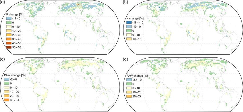
W. de Oliveira Garcia et al.: Impacts of enhanced weathering                                                              2109

worldwide soils (6.8 × 10⁹ ha of land) have unfavorable soil     geogenic P supply given by observation-based estimates of
conditions for agricultural production (Fischer et al., 2001).   soil inorganic labile P and organic P (Yang et al., 2014a);
Therefore, we assess if applications of rock mineral-based P     observation-based estimates of P release (Hartmann et al.,
sources could close eventual nutritional gaps in an environ-     2014) from weathering corrected to future temperature in-
ment with natural N supply (N-limited) and with N fertil-        creases, since the uncertainty in the future hydrological cycle
ization (N-unlimited), using a global afforestation scenario.    is too high (Goll et al., 2014); and estimated atmospheric P
In addition, we investigate the effects of coupling nutrient-    depositions from Wang et al. (2017) to derive the potential
supplying (EW) to nutrient-demanding (AR and BG) land-           geogenic P deficits (i.e, the P gap) during the 21st century.
based NETs by focusing on the efficiency of different up-        Since the geogenic P supply cannot cope with N-stock-based
per limits of basalt powder to supply nutrients. We hypothe-     P demand from the different AR scenarios within P gapped
size that large-scale EW deployment potentially changes soil     areas, the biomass production and biomass C sequestration,
texture. Therefore, threshold values for impacts on soil hy-     predicted by the AR scenarios, will be lower. Based on the
draulic conductivity and plant-available water will be deter-    amount of missing P, we estimated the C-stock reduction
mined.                                                           within P gapped areas by using stoichiometric C : P ratios.
                                                                 The C : P ratios were derived from simulated C-stock con-
                                                                 tent (Kracher, 2017) and inferred N-stock-based P demand.
2   Methods                                                         Necessary Mg, Ca, and K supply for balanced tree nu-
                                                                 trition based on P supply was derived from N-stock-based
Since phosphorus (P) is a limiting nutrient in a wide range of   Mg, Ca, and K additional demand normalized to the N-stock-
ecosystems (Elser et al., 2007), we performed a P budget for     based additional P demand (Fig. 1). The nutrient demand of
an N-stock-based P demand from an AR scenario consider-          bioenergy grass was estimated based on stoichiometric P : N
ing natural N supply (hereafter N-limited) and N fertilization   and K : N ratios, used in Bodirsky et al. (2012), for minimum
(hereafter N-unlimited). We selected two N supply scenar-        and maximum exported N proportional to harvest rates of the
ios since the related P demand is proportional to biomass N      1995–2090 period obtained from the agricultural production
stock, but in the main text we discuss only the N-limited AR     model MAgPIE (Fig. 1). Later on, the necessary amount of
scenario. We estimated the balanced supply of Mg, Ca, and K      rock to cover the P gaps of the AR scenario and to resupply
for each supplied P based on ideal Mg, Ca, and K demand of       the nutrients exported by BG harvest was estimated (Fig. 1).
AR derived from databases of biomass nutrient content. Bal-      In addition, the potential impact of deploying rock powder
anced nutrient supply is necessary to avoid shift of growth      into the topsoil hydrology was modeled.
limitation to other nutrients, which can occur according to
Liebig’s law (von Liebig and Playfair, 1843). Shift of growth    2.1     Global land-system model output
limitation to other nutrients is observed for some US forests
that changed from an N-limited to a P-limited system after an    2.1.1    Afforestation and reforestation
increase in atmospheric N deposition (Crowley et al., 2012).
Based on minimum and maximum harvest rates of bioenergy          The idealized simulations for the AR system from
grass (BG), we estimated the related P and K export by har-      Kracher (2017) performed by the land surface model JS-
vest from the fields. We decided on these nutrients for BG       BACH (Reick et al., 2013) for RCP4.5 were used (Thomson
since crops require large amounts of K and P, once N de-         et al., 2011). The RCP4.5 scenario assumes that the emis-
mand is covered. The amount of rock powder required for en-      sions peak is around 2040 and considers that forest lands ex-
hanced weathering (EW) to cover projected P gaps and to re-      pand from their present-day extent (Thomson et al., 2011).
plenish exported nutrients was estimated. The projected im-      The coupled terrestrial nitrogen–carbon cycle model assumes
pacts on soil hydrology due to EW deployment were carried        N-unlimited and N-limited conditions and considers harvest
out by pedotransfer functions since they are used to estimate    rates and transitions between different anthropogenic and
soil hydraulic properties (Schaap et al., 2001; Whitfield and    natural land cover types (Hurtt et al., 2011) for a Gaus-
Reid, 2013; Wösten et al., 2001) and such approximations         sian grid of approximately 2◦ × 2◦ resolution. Accounting
have proven to be a suitable approach (Vienken and Dietrich,     for the N cycle reduces the uncertainty in atmospheric car-
2011).                                                           bon sequestration prediction by AR models (Zaehle and Dal-
   The additional AR P demand, obtained for the 21st cen-        monech, 2011). In JSBACH, the N supply for plants is con-
tury for an N-unlimited and N-limited AR scenario (Kracher,      trolled by competition between plants and decomposing mi-
2017), was approximated by stoichiometric P : N ratios for       crobes, while other numerical models prioritize immobiliza-
mean and range (5th and 95th percentiles), which is a sim-       tion or plant growth (Achat et al., 2016).
ilar approach to that of Sun et al. (2017). The ratios were         The net primary productivity (NPP) calculation was based
derived from databases of hardwood and softwood (Pardo et        on atmospheric CO2 concentrations, stomatal conductance,
al., 2005) and foliar biome-specific nutrient content (Vergutz   and water availability. JSBACH considers mass conserva-
et al., 2012). We then compared the inferred P demand to         tion, a supply–demand ansatz, and fixed C : N ratios (Goll

www.biogeosciences.net/17/2107/2020/                                                    Biogeosciences, 17, 2107–2133, 2020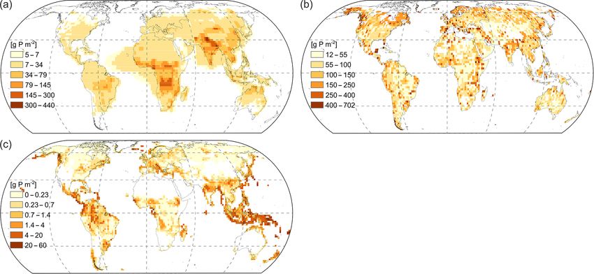
2110                                                               W. de Oliveira Garcia et al.: Impacts of enhanced weathering

Figure 1. Schematic steps and datasets used to derive geogenic nutrient demand from simulated biomass changes; P gaps; reduced C
sequestration; and Ca, K, and Mg supply for balanced tree nutrition. Black colors: outputs from land surface model JSBACH and agricultural
production model MAgPIE. Yellow colors: stoichiometric Mg : N, Ca : N, K : N, and P : N ratios used to obtain the N-stock-based nutrient
demand. Red colors: N-stock-based P, Mg, Ca, and K demand for wood and leaf (AR) or N harvest export-based P and K demand (BG).
Green colors: nutrient supply from geogenic sources (atmospheric P deposition and different soil P pools) or from enhanced weathering.
Blue colors: derived P gap for AR; derived stoichiometric C : P, Mg : P, Ca : P, and K : P ratios; P-based C-fixation reduction; and P-based
Mg, Ca, and K supply for balanced tree nutrition. Purple colors: related EW deployment impacts on soil hydrology estimated by pedotransfer
functions. AR: afforestation–reforestation; BG: bioenergy grass.

et al., 2012). The coupled terrestrial nitrogen–carbon cycle            sidered future CO2 increase leading to CO2 fertilization, and
model was selected since it (i) considered forest regrowth on           (v) explicitly considered large-scale afforestation.
abandoned croplands (which in the long term become acidic                  We retrieved the annual changes in N and C content of
and consequently favor leaching of nutrients and heavy met-             different pools, i.e., wood (above and below ground, also in-
als; Hesterberg, 1993), (ii) considered natural shift in natural        cluding litter) and foliar (above and below ground, also in-
vegetation, (iii) considered a natural N supply scenario (N-            cluding litter) for temperate, cold, tropical, and subtropical
limited) and an N-fertilized scenario (N-unlimited), (iv) con-          plant functional types climate growing forests and shrubs for
                                                                        the years 2006–2099 and annual model output.

Biogeosciences, 17, 2107–2133, 2020                                                           www.biogeosciences.net/17/2107/2020/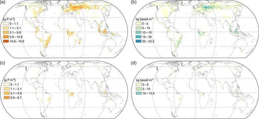
W. de Oliveira Garcia et al.: Impacts of enhanced weathering 2111
2.1.2 Biomass production from bioenergy grass
Simulations of BG nutritional needs from the agricultural
production model MAgPIE, a framework for modeling
global land systems (Dietrich et al., 2018; Lotze-Campen
et al., 2008; Popp et al., 2010), were used. The objective of
MAgPIE is to minimize total costs of production for a given
amount of regional food and bioenergy demand and a given
climate target (here RCP4.5 to correspond to the AR simu-
lations). In its biophysical core, the yields in the model are
based on LPJmL (Bondeau et al., 2007; Beringer et al., 2011;
Müller and Robertson, 2013), a dynamic global vegetation
model, which is designed to simulate vegetation composition
and distribution for both natural and agricultural ecosystems.
At the starting point of the simulation, the LPJmL bioen-
ergy grass yields have been scaled using agricultural land
use intensity levels (Dietrich et al., 2012) for different world
regions accounting for the yield gap between potential and
observed yields for the period 1995–2005. For the future
yields (2005–2090), the development is then driven by in-
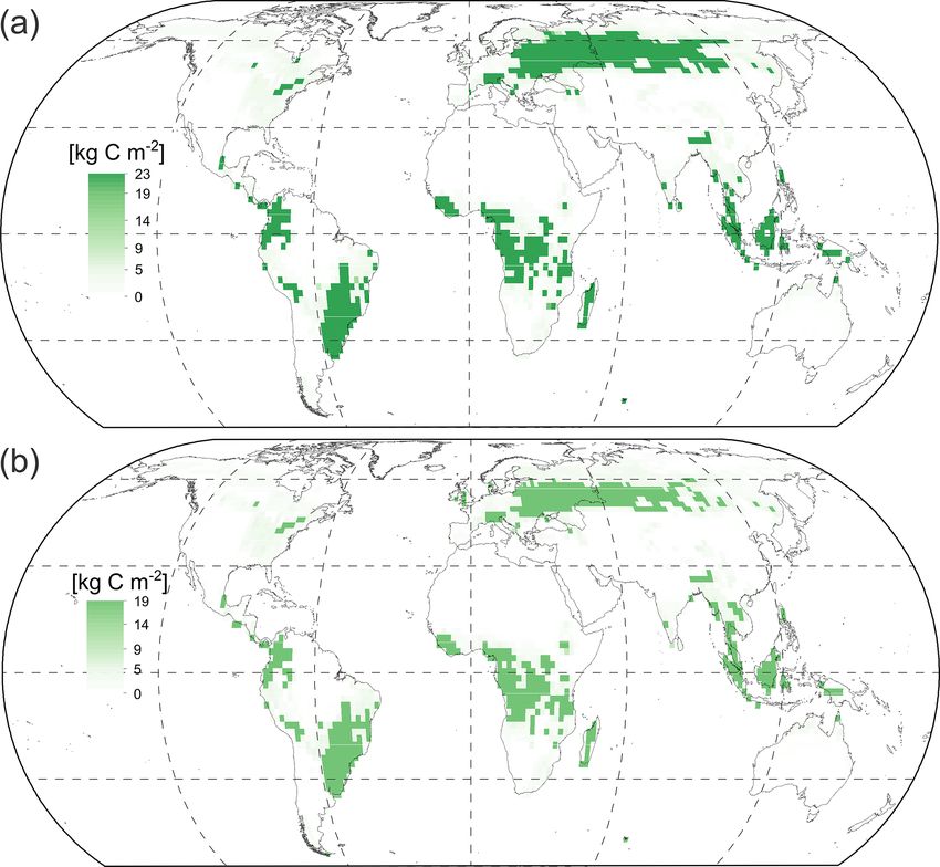
vestments into yield-increasing technologies (Dietrich et al., Figure 2. Carbon sequestered in different afforestation–
2014) based on the socioeconomic boundary conditions of reforestation scenarios for the 21st century period (2006–2099)
for an RCP4.5 scenario, according to Kracher (2017). (a) For an
the system.
N-unlimited AR scenario the global C sequestration is 224 Gt C.
The MAgPIE output had a frequency of 10 a, and the (b) For an N-limited AR scenario the global C sequestration is
global minimum and maximum of each output year were 190 Gt C. © ESRI.
taken to obtain the potential bioenergy grass minimum
(0.7 kg m−2 a−1 ) and maximum (3.6 kg m−2 a−1 ) harvest
rate for the simulation period for the areas with bioenergy (above and below ground, including litter) and foliar (above
plantations. and below ground, including litter).
The P, Mg, Ca, K, and N content of leaves obtained from
2.2 Nutrient demand
a global leaf chemistry database (Vergutz et al., 2012) was
2.2.1 Afforestation and reforestation used to derive the Mg : N, Ca : N, K : N, or P : N ratios (Ta-
ble 1), which were already biome classified. For wood, the
The P, Mg, Ca, and K additional demand is defined as the tree chemical composition database of US forests (Pardo et
amount of P, Mg, Ca, and K needed to realize the state of al., 2005) was used in order to derive the global ratios, which
ecosystem N variables in each grid cell and year according were assumed to represent the chemical composition of all
to JSBACH output (Fig. 1). It was estimated from the spa- biomes (Table 1).
tially explicit information on average forest N content of each The AR C content (Fig. 2) from Kracher (2017) and the
stock and plant functional type for an N-unlimited and an N- resulting N-stock-based Mg, Ca, and K demand were nor-
limited AR scenario from Kracher (2017). Since P limits for- malized by the N-stock-based P demand to estimate the mean
est growth in a wide range of ecosystems (Elser et al., 2007), and range of the C : P, Mg : P, Ca : P, and K : P ratios of each
we performed a P budget for each AR scenario. The ideal grid cell. The stoichiometric C : P, Mg : P, Ca : P, and K : P
P, Mg, Ca, and K biomass additional demands were based ratios were used to derive the C-fixation reduction due to P
on the difference in the simulated change in N pools at that deficiencies and the necessary Mg, Ca, and K supply for a
time with respect to the simulation year of 2006 multiplied balanced biomass nutrition based on supplied P (Fig. 1).
by their corresponding Mg : N, Ca : N, K : N, or P : N ratios
(rij ) and were calculated following Eq. (1): 2.2.2 Biomass production from bioenergy grass
Xn
1Mpool,i = 1Nij × rij , (1) The BG yield was obtained by the spatially explicit harvest
j =1
rates within a grid cell for an output frequency of 10 a and a
where 1Mpool,i (kg m−2 a−1 ) is the average N-stock-based period of 95 a (1995–2090). The minimum 0.7 and maximum
Mg, Ca, K, or P demand for a given time in the future simula- 3.6 kg m−2 a−1 harvest rates were used. With the information
tion time range (2007–2099) within a cell for biome i. 1Nij on exported N by each harvest rate, the exported K or P from
(kg m−2 a−1 ) is the average N-stock change in pool j . The cultivation fields (Eq. 2) was estimated based on the P : N and
number of N pools is n. The N pools considered are wood K : N stoichiometric ratios used in Bodirsky et al. (2012). We
www.biogeosciences.net/17/2107/2020/ Biogeosciences, 17, 2107–2133, 2020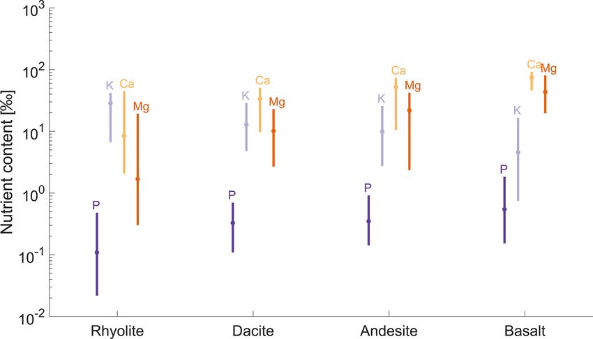
2112 W. de Oliveira Garcia et al.: Impacts of enhanced weathering
Table 1. Stoichiometric parameters for different pools and biomes used in this study.
Biome Tropical evergreen Tropical deciduous Temperate evergreen
Leafb Mean SD n 5th 95th Mean SD n 5th 95th Mean SD n 5th 95th
percentile percentile percentile percentile percentile percentile
C:N (–) 29.72 15.01 4 16.33 46.49 26.96a 10.53a 171a 14.50a 46.7a 49.11 12.15 8 33.54 65.69
P:N 0.06 0.02 59 0.04 0.10 0.07 0.03 43 0.04 0.13 0.09 0.03 23 0.05 0.13
K:N 0.97 0.80 2 0.46 1.48 1.26 0.93 22 0.23 2.45 0.47 0.09 12 0.33 0.58
Ca : N 2.73 3.44 2 0.54 4.91 1.55 0.78 22 0.52 2.90 0.73a 0.67a 150a 0.16a 1.94a
Mg : N 0.40 0.52 2 0.07 0.73 0.37 0.29 22 0.10 0.83 0.21a 0.21a 115a 0.05a 0.66a
Woodc Mean SD n 5th 95th Mean SD n 5th 95th Mean SD n 5th 95th
percentile percentile percentile percentile percentile percentile
C:N (–) 235 244 9 56 610 235 244 9 56 610 235 244 9 56 610
P:N 0.15 0.20 684 0.04 0.30 0.15 0.20 684 0.04 0.30 0.15 0.20 684 0.04 0.30
K:N 0.60 0.40 700 0.20 1.20 0.60 0.40 700 0.20 1.20 0.60 0.40 700 0.20 1.20
Ca : N 1.80 1.30 705 0.40 4.30 1.80 1.30 705 0.40 4.30 1.80 1.30 705 0.40 4.30
Mg : N 0.20 0.10 681 0.10 0.40 0.20 0.10 681 0.10 0.40 0.20 0.10 681 0.10 0.40
Biome Temperate deciduous Shrubs raingreen Shrubs deciduous
Leafb Mean SD n 5th 95th Mean SD n 5th 95th Mean SD n 5th 95th
percentile percentile percentile percentile percentile percentile
C:N (–) 55.30 12.02 2 47.65 62.95 26.31 6.83 2 21.97 30.65 26.96a 10.53a 171a 14.5a 46.70a
P:N 0.08 0.03 32 0.04 0.13 0.07 0.01 2 0.06 0.08 0.08a 0.05a 662a 0.04a 0.16a
K:N 0.43 0.13 23 0.24 0.61 0.38 0.02 2 0.37 0.39 0.59a 0.45a 207a 0.24a 1.50a
Ca : N 0.73a 0.67a 150a 0.16a 1.94a 0.44 0.08 2 0.39 0.50 0.73a 0.67a 150a 0.16a 1.94a
Mg : N 0.21a 0.21a 115a 0.05a 0.66a 0.09 0.04 2 0.06 0.12 0.21a 0.21a 115a 0.05a 0.66a
Woodc Mean SD n 5th 95th Mean SD n 5th 95th Mean SD n 5th 95th
percentile percentile percentile percentile percentile percentile
C:N (–) 235 244 9 56 610 235 244 9 56 610 235 244 9 56 610
P:N 0.15 0.20 684 0.04 0.30 0.15 0.20 684 0.04 0.30 0.15 0.20 684 0.04 0.30
K:N 0.60 0.40 700 0.20 1.20 0.60 0.40 700 0.20 1.20 0.60 0.40 700 0.20 1.20
Ca : N 1.80 1.30 705 0.40 4.30 1.80 1.30 705 0.40 4.30 1.80 1.30 705 0.40 4.30
Mg : N 0.20 0.10 681 0.10 0.40 0.20 0.10 681 0.10 0.40 0.20 0.10 681 0.10 0.40
a Values obtained from all biomes. b Stoichiometric ratios derived from a global leaf chemistry database (Vergutz et al., 2012). c Stoichiometric ratios derived from a US softwood and hardwood database (Pardo et al., 2005). See
file “S2.xlsx” in the Supplement for used database.
have chosen these nutrients since crops require large amounts lation to minimize distortions of location (Pontius, 2000).
of K and P, once N demand is covered. The nearest-neighbor interpolation method reliably retains
The simulated forests from the AR scenario are perennial, the overall proportions of an original fine-resolution map
unlike bioenergy grasses which are completely harvested (Christman and Rogan, 2012). As the uncertainty in which P
regularly due to their use as biomass feedstock for BECCS. pool is available for long-term plant nutrition is high (John-
Thus, the natural system’s nutrient supply is insufficient for son et al., 2003), two scenarios for soil P supply were in-
maintaining successive and constant yields, and the nutrients vestigated: scenario one, considering P from weathering and
exported by harvest need to be replenished (Cadoux et al., atmospheric P deposition, and scenario two, the same as sce-
2012) to maintain high yields. The exported nutrients were nario one plus inorganic labile P and organic P (Yang et al.,
calculated following Eq. (2): 2014a).
The atmospheric dry and wet P deposition rates were taken
Biox = rx × Nharvest , (2) from simulation outputs for the 2006–2013 period and for
the years 2030, 2050, and 2099 for an RCP4.5 scenario for a
where Biox corresponds to the exported nutrient P or K grid cell size of 1◦ (Wang et al., 2017). The simulations were
(kg m−2 a−1 ) by harvest. The P : N or K : N stoichiometric based on P emissions of sea salt, dust, biogenic aerosol parti-
ratio used in Bodirsky et al. (2012) is rx . Nharvest is the ex- cles, and P emitted by combustion processes and performed
ported N for a minimum 0.7 or a maximum 3.6 kg m−2 a−1 by the global aerosol chemistry–climate model LMDz-INCA
harvest rate. The harvest rate value was based on the MAg- (see Wang et al., 2017, for a detailed description of model
PIE output for each grid cell, representing the minimum and and model assumptions). The simulation gaps were closed
maximum projected global harvest rate for a period of 95 a. by linear regression, and the cumulative atmospheric P depo-
sition was calculated by summing up the deposition rate of
2.3 Geogenic P supply for AR
each cell for the 2006–2099 period according to Eq. (3):
The geogenic P source databases have different spatial res-
olutions (Table 2); we resampled each of them to a coarser X2099
2◦ × 2◦ spatial resolution field by nearest-neighbor interpo- Ptot = P,
i=2006 i
(3)
Biogeosciences, 17, 2107–2133, 2020 www.biogeosciences.net/17/2107/2020/W. de Oliveira Garcia et al.: Impacts of enhanced weathering 2113
Table 2. Geogenic P sources used for each geogenic P supply scenario.
P source Resolution Geogenic P supply Geogenic P supply Reference
scenario one scenario two
Soil organic P and inorganic labile P 0.5◦ X Yang et al. (2014a)
Atmospheric P deposition 1◦ X X Wang et al. (2017)
P from weathering 1 km2 X X Hartmann et al. (2014)
where Ptot (kg m−2 ) is the cumulative atmospheric P deposi- wood and leaves derived from the N-limited and N-unlimited
tion of the 2006–2099 period (Fig. 3a). P (kg m−2 a−1 ) is the AR scenario N stock as described in Sect. 2.2.1 is rC .
atmospheric P deposition of each year i within a grid cell. The Mg, Ca, and K necessary supply for balanced biomass
The total soil P map from Yang et al. (2014a) was used to nutrition (Mx (kg m−2 )) should be proportional to the sup-
estimate the projected long-term available P in the soil sys- plied P (PEW (kg m−2 )) and was calculated following Eq. (6):
tem (Fig. 3b). The total P supply by weathering for the 21st
century (2006–2099) was based on Hartmann et al. (2014)
maps (Fig. 3c) that depict the chemical weathering as a func- Mx = rx × PEW , (6)
tion of runoff and lithology, corrected for temperature and
with PEW being equal to the projected Pgap since it is covered
soil thickness (Hartmann et al., 2014) and calibrated on 381
by P from enhanced weathering according to Eq. (7).
catchments in Japan (Hartmann et al., 2009). A relationship
between air temperature and weathering rate was used, which PEW = Pgap , (7)
was derived from reconstructed weathering rates and differ-
ent climate change scenarios for the recent past (1860–2005) where rx is the used stoichiometric ratio Mg : P, Ca : P, or
using the weathering model applied here. The relationship K : P obtained by normalizing the N-stock-based additional
in which P weathering increases by 9 % per 1 ◦ C increase Mg, Ca, and K demand to the N-stock-based additional P
(Goll et al., 2014) implicitly accounts for changes in soil demand.
hydrology, without accounting for P concentration changes
in primary and secondary P minerals. Due to the large un- 2.5 Enhanced weathering Mg, K, Ca, and P potential
certainties in projected changes in soil hydrology, we omit- supply
ted a more detailed representation of hydrological effects on
To cover the potential of different igneous rocks for EW
weathering.
strategies, rhyolite and dacite (acidic rocks), andesite (in-
2.4 Estimating geogenic P gap; related C-fixation termediate rock), and basalt (basic rock) were selected to
reduction; and balanced Mg, Ca, and K supply for project necessary amounts to cover P gaps from the AR sce-
AR narios. Data on macronutrient concentrations (Mg, Ca, K, P)
in weight percent within these rocks were downloaded from
The potential P gap (Pgap (kg m−2 )) was estimated as the the EarthChem web portal (Fig. 4; http://www.earthchem.
difference between the mean and range (95th and 5th per- org, last access: 14 July 2017). The data were selected for
centiles) of additional P demand estimated from the N stock rocks categorized as rhyolite, dacite, andesite, and basalt, ne-
for the two different AR scenarios (see Sect. 2.2.1) and the glecting intermediate compositions between different litho-
geogenic P supply from the different supply scenarios (Psup types (i.e., a trachybasalt that has its chemical composition
(kg m−2 )) within the cover fraction for a grid cell of biome lying between trachyte and basalt). Rocks that were under
i (fi (–)), for the 21st century (2006–2099) according to any metamorphism grade (e.g., metabasalt) were neglected
Eq. (4): because metamorphism can change rock mineralogy. We ne-
glected rocks known to have a high content of minerals rich
Pgap = Psup × fi − 1Ppool,i . (4) in trace elements (e.g., an alkali basalt can have a P con-
centration > 3000 ppm (Porder and Ramachandran, 2013),
The plant C-fixation reduction was estimated based on the P but it is rich in olivine (John, 2001; Irvine and Baragar,
gap and calculated following Eq. (5): 1971), which contains elevated concentrations of nickel and
chromium (Edwards et al., 2017)). Nickel and chromium are
C = rC × Pgap , (5) trace elements problematic for agriculture (Edwards et al.,
2017). Thus, following the classification criteria, the num-
where C (kg m−2 ) is the reduced plant C fixation due to the bers of selected data to calculate descriptive statistics for
projected P gap. The used stoichiometric C : P ratio based on Mg, Ca, K, and P content within rocks were 2985 chemi-
the mean and range (5th and 95th percentiles) chemistry for cal analyses for rhyolite, 3008 chemical analyses for dacite,
www.biogeosciences.net/17/2107/2020/ Biogeosciences, 17, 2107–2133, 20202114 W. de Oliveira Garcia et al.: Impacts of enhanced weathering
Figure 3. Different sources of geogenic P. (a) Cumulative atmospheric P deposition for 2006–2099 according to Wang et al. (2017). (b) Total
inorganic labile P and organic P in the soil up to a depth of 0.5 m according to Yang et al. (2014a). (c) Cumulative weathering P release for
the 21st century (2006–2099) based on Hartmann et al. (2014), accounting for weathering rate changes related to temperature increase (Goll
et al., 2014). © ESRI.
(157 ppm) and 95th (1833 ppm) percentiles), as basalt is
abundant worldwide (Amiotte Suchet et al., 2003; Börker et
al., 2019) and has a high P content compared to acidic and in-
termediate rocks (Porder and Ramachandran, 2013). Median
P concentration can be > 3000 ppm for alkali basalts, but for
a broader basalt classification that considered 97 895 sam-
ples, it can be 916 ppm (Porder and Ramachandran, 2013).
The necessary mass of rock powder to supply macronutrients
(Mg, Ca, K, or P) was calculated following Eq. (8):
Mex
Rd = , (8)
fnut
Figure 4. Statistical data of major element concentration in rocks
with median values (filled circles) and range (5th and 95th per-
centiles; whiskers). Values from EarthChem web portal (http:// where Rd (kg rock m−2 or kg rock m−2 a−1 ) represents the
www.earthchem.org, last access: 14 July 2017). The numbers of mass of a rock type to cover AR or BG nutritional needs,
chemical analyses used to calculate the descriptive statistics were Mex (kg m−2 or kg m−2 a−1 ) is the mass of required nutrient
2985 chemical analyses for rhyolite, 3008 chemical analyses for
for AR or BG (e.g., P to cover a Pgap obtained by Eq. 4),
dacite, 11 099 chemical analyses for andesite, and 23 816 chemical
analyses for basalt.
and fnut (–) is the median and range (5th or 95th percentile)
fractions of interest nutrient within the selected rock.
However, the potential nutrient supply by EW for different
amounts of rock powder being deployed was also estimated
11 099 chemical analyses for andesite, and 23 816 chemical
following Eq. (9):
analyses for basalt.
The nutrient supply was estimated assuming complete
rock powder dissolution in the system considering the me- Nutin = Mrock × fnut , (9)
dian and range (5th or 95th percentile) of chemical com-
position. The duration of complete rock powder dissolu-
tion varies depending on the grain size (i.e., 1 a for grain where Nutin (kg m−2 or kg m−2 a−1 ) represents the macronu-
sizes between 0.6 and 90 µm for basalt; Strefler et al., 2018). trient input by dissolving a chosen rock. Mrock (kg rock m−2
The results and discussion will focus on basalt rock pow- or kg rock m−2 a−1 ) is the mass of rock added to the natural
der considering median P values (500 ppm) and range (5th system.
Biogeosciences, 17, 2107–2133, 2020 www.biogeosciences.net/17/2107/2020/W. de Oliveira Garcia et al.: Impacts of enhanced weathering 2115
2.6 Related impacts on soil hydrology from enhanced with
weathering deployment
θ1500t = −0.024 × S + 0.487 × C + 0.006 × OM
+ 0.005 × (S × OM) − 0.013 (C × OM)
Large-scale deployment of rock powder on soils is expected
to influence its texture. The deployed amount and texture + 0.068 (S × C) + 0.031, (15)
of rock powder will somehow affect hydraulic conductiv- θ33t = −0.251 × S + 0.195 × C + 0.011 × OM
ity, water retention capacity, and specific soil surface area. + 0.006 × (S × OM) − 0.027 × (C × OM)
Pedotransfer functions (PTFs) are used to estimate soil hy-
draulic properties (Schaap et al., 2001; Whitfield and Reid, + 0.452 (S × C) + 0.299, (16)
2013; Wösten et al., 2001), and such approximations have θ(S−33)t = 0.278 × S + 0.034 × C + 0.022 × OM
proven to be a suitable approach (Vienken and Dietrich, − 0.018 × (S × OM) − 0.027 × (C × OM)
2011). PTFs make use of statistical analysis (Saxton and
− 0.584 × (S × C) + 0.078, (17)
Rawls, 2006; Wösten et al., 2001), artificial neural networks,
ln (1500) − ln (33) −1
and other methods applied to large soil databases of mea-
λ= , (18)
sured data (Wösten et al., 2001). The equations from Sax- ln (θ33 ) − ln (θ1500 )
ton et al. (1986) performed the best estimations of soil hy-
draulic properties (Gijsman et al., 2002). Later on, Saxton where S and C, respectively, represent the soil texture corre-
and Rawls (2006) improved Saxton et al. (1986) PTFs, and sponding to sand and clay diameters (wt %); OM is the soil
they are used to estimate the effects on soil hydraulic proper- organic matter (wt %); and the moisture (wt %) is estimated
ties due to deployment of basalt powder (Eqs. 10–18). by θ1500 and θ33 , respectively, representing the soil moisture
The potential changes in soil hydraulic properties, due to for a pressure head of −1500 kPa (R 2 = 0.86) and −33 kPa
the application of a fine basalt texture (15.6 % clay, 83.8 % (R 2 = 0.63). θ(S−33) and θS , respectively, correspond to the
silt, and 0.6 % fine sand) or a coarse basalt texture (15.6 % 0 kPa to −33 kPa moisture (R 2 = 0.36), and to the saturated
clay, 53.8 % silt, and 30.6 % fine sand), were estimated as (0 kPa) moisture (R 2 < 0.25). KS (mm h−1 ) represents the
a function of rock powder deployment for soils correspond- saturated soil hydraulic conductivity, and λ is the slope of the
ing to P gap areas from the N-unlimited AR scenario. Ac- logarithmic tension–moisture curve. The numbers in front of
cording to the international organization for standardization, each described variable are regression coefficients (Saxton
the synthetic materials can be classified according to their and Rawls, 2006).
grain sizes; therefore, here the clay comprises grain diam- The initial hydrologic properties of topsoil were estimated
eters ≤ 2 µm, silt comprises grain diameters 2–63 µm, and for a depth of 0.3 m, as it is the average depth at which
fine sand comprises grain diameters 63–200 µm (ISO 14688- usual machinery can homogeneously mix topsoil (Fageria
1:2002, 2002), but since full dissolution is assumed, the and Baligar, 2008). Greater depths can be reached but under
ground basalt fine sand encompasses grain sizes of diame- higher energy and labor costs (Fageria and Baligar, 2008).
ter 63–90 µm remaining within the ISO 14688-1:2002 clas- The global dataset of derived soil properties (Batjes, 2005),
sification. The N-unlimited AR scenario was selected since which had textural information (sand, silt, and clay content)
it would have the highest P deficiencies requiring more rock for shallow soil depths (0.3 m), was used. The raster had a
powder to cover the P gaps (i.e., it represents the maximum resolution of 0.5◦ , and the soil properties for the interest ar-
effect). The estimations are for a homogeneous mixture of eas of biomass growth limitation (the same as the areas dis-
rock powder and topsoil depth of 0.3 m. Downward trans- played in Fig. S7a in the Supplement) were included by a
port of fine-grained material is neglected for simplification. spatial join (using Esri ArcMap 10.8). The nutrient-deficient
The considered values represent upper limits of rock powder areas encompass soils of different textures and organic mat-
application. The impacts on plant-available water (PAW) is ter content, which had their initial KS estimated separately
given by the difference between water content at a pressure based on Eq. (14). The sum of clay, silt, and sand fractions
head of −33 kPa (Eq. 11) and −1500 kPa (Eq. 10), while the within each cell should always be a unity and were corrected
impact on soil hydraulic conductivity is given by (Eq. 14) when necessary by Eq. (19):
(Saxton and Rawls, 2006): (Gini × Msoil_cell )
Gcor = P , (19)
(Gini × Msoil_cell )
θ1500 = θ1500t + (0.14 × θ1500t − 0.02), (10) with
2
θ33 = θ33t + 1.283 × (θ33t ) − 0.374 × (θ33t − 0.015), (11) Msoil_cell = Vcell × ρbulk_cell , (20)
θ(S−33) = θ(S−33)t + (0.636 × θ(S−33)t − 0.107), (12)
where Gini represents the initial topsoil texture (sand, silt,
θS = θ33 + θ(S−33) − 0.097 × S + 0.043, (13) and clay content) of a specific raster cell (–). Vcell (km3 ) is
KS = 1930 × (θS − θ33 )(3−λ) , (14) the raster cell volume obtained by multiplying the area (km2 )
www.biogeosciences.net/17/2107/2020/ Biogeosciences, 17, 2107–2133, 20202116 W. de Oliveira Garcia et al.: Impacts of enhanced weathering
to the soil depth of 0.3 × 10⁻³ km. ρbulk_cell (kg km−3 ) is the 3 Results
raster cell topsoil bulk density. Msoil_cell (kg) is the total soil
mass of a raster cell. Gcor (–) is the corrected soil texture 3.1 Afforestation and reforestation P gaps and
(sand, silt, and clay content). enhanced weathering as nutrient source
The necessary rock powder mass was estimated by Eq. (8)
to close the Pgap obtained by Eq. (4). The effect of basalt The global C sequestration for the N-limited AR scenario
powder application in soil KS and PAW was estimated by as- is 190 Gt C, while for the N-unlimited AR scenario it is
suming a homogeneous mixture between applied basalt pow- 34 Gt C higher. The AR model from Kracher (2017) shows
der and topsoil. The changes in initial soil organic matter an increase in biomass production in tropical and temper-
(SOM) concentration within a raster grid cell were obtained ate zones (Fig. 2). The results only focus on the N-limited
by normalizing the SOM to the sum of applied basalt mass, scenario since it considered natural N supply, but the re-
mass of soil, and initial SOM mass by Eq. (21). This was nec- sults for the N-unlimited scenario are presented in the Sup-
essary since the SOM concentration at the moment of basalt plement (Sect. Bii). The calculated P budgets according to
deployment would have a relative decrease compared to ini- Eq. (4) for the AR time of 2006–2099 (Fig. 5) considered
tial SOM concentration: different geogenic supply scenarios (scenario one – P from
OMcell weathering and atmospheric P deposition; scenario two –
OMc = × 100, (21) the same as scenario one plus inorganic labile P and or-
Mb_cell + Msoil_cell + OMcell
ganic P) and the average and range of the N-stock-based P
with demand (calculated following Eq. 1) for the AR simulation
OMcell = OMwt % × Msoil_cell , (22) from Kracher (2017).
The ideal P biomass additional demand (calculated from
where OMc (wt %) is the corrected soil organic matter con- Eq. 1) to sequester 190 Gt C (N-limited AR scenario)
tent, OMcell (kg) is the organic matter mass within the raster amounts to 200 Mt P on a global scale for a mean wood and
cell. Mb_cell and Msoil_cell , both in kilograms, are the mass of leaves P content; for the 5th and 95th percentile, the esti-
basalt and mass of soil for a specific raster cell. mated P demand would be 71 and 345 Mt P, respectively.
The impacts on soil texture by rock powder application The P budget (estimated from Eq. 4) for geogenic P supply
considered the textures of applied basalt mass added to the scenario one suggests that P deficiency areas are distributed
initial soil mass by Eq. (23). A content of 15.6 % clay, 83.8 % around the world but with more frequent occurrences in the
silt, and 0.6 % fine sand for fine basalt powder and 15.6 % Northern Hemisphere (Fig. 5a) and the P gaps can poten-
clay, 53.8 % silt, and 30.6 % fine sand for a coarse basalt tially reach up to ∼ 17 g P m−2 (∼ 4–∼ 30 g P m−2 for the
powder was assumed. 5th and 95th percentiles of wood and leaves chemistry; Ta-
ble 3) or a global P gap of ∼ 77 Mt P (∼ 9–181 Mt P2 for the
5th and 95th percentiles of wood and leaves chemistry; Ta-
Gini × Msedcell + Mbcell × Gbasalt
Gbs = P , (23) ble 3). However, for geogenic P supply scenario two, the P
Gini × Msedcell + Mbcell × Gbasalt
deficiency areas are predominantly located in the Southern
where Gbasalt corresponds to the texture fractions of the fine Hemisphere (Fig. 5c) and the P gaps can potentially reach up
or coarse basalt powder. Gbs corresponds to the texture frac- to ∼ 7 g P m−2 (∼ 2–∼ 12 g P m−2 for the 5th and 95th per-
tions of the resulting mixture of basalt plus soil. Thus, the centiles of wood and leaves chemistry; Table 3) or a global
texture fractions of the resulting mixture of basalt plus soil P gap of ∼ 10 Mt P (1–∼ 35 Mt P2 for the 5th and 95th per-
obtained by Eq. (23) were replaced within Eqs. (15–17) centiles of wood and leaves chemistry; Table 3).
to estimate the impacts on soil hydraulic conductivity by The P and N limitations cause an average C reduction of
Eq. (14) and PAW by subtracting the outcome from Eq. (11) 47 % for the geogenic P supply scenario one and 19 % for the
to the outcome from Eq. (10), with clay size (grains > 1 and geogenic P supply scenario two (obtained by accounting for
< 3.9 µm) being the finest grain size we can consider. the C reduction from N limitation, which is 34 Gt C plus the
Besides texture and organic matter, intrinsic grain prop- C reduction from Table 3, and then normalizing by the global
erties (e.g., the shape of grains and pores, tortuosity, spe- sequestration for the N-unlimited scenario of 224 Gt C) or
cific surface area, and porosity) should be considered (Bear, ∼ −1.1 and ∼ −0.5 Gt C a−1 , respectively. In some areas,
1972). The equations from Beyer (1964) are based on the the C sequestration can be reduced by up to 100 % compared
nonuniformity of grain size distribution and density of the to the predicted C sequestration of the AR models (Fig. 6).
grain packing to estimate soil properties. Carrier (2003) uses Accounting for N and P limitation on AR suggests that the
information on the particle grain size distribution, the parti- biomass production will be affected, consequently decreas-
cle shape, and the void ratio in his equations to estimate soil ing the C sequestration potential of AR strategies (Table 3
properties. However, such detailed information on a global and Fig. 6). Therefore, supplying the demanded P would pos-
scale is missing, making Beyer (1964) and Carrier (2003) itively contribute to biomass reaching the predicted growth of
equations not applicable to our analysis. the specific AR scenario.
Biogeosciences, 17, 2107–2133, 2020 www.biogeosciences.net/17/2107/2020/W. de Oliveira Garcia et al.: Impacts of enhanced weathering 2117
Figure 5. Areas with potential P gap for the nutrient budget of the N-limited AR scenario (after 94 a of simulation), assuming P concentrations
within foliar and wood material corresponding to mean values (Table 1). (a) Geogenic P supply scenario one (geogenic P from weathering
plus atmospheric P deposition as source of P). (b) Basalt deployment necessary to close P gaps from P budget scenario of Fig. 5a. (c) Geogenic
P supply scenario two (geogenic P from soil inorganic labile P and organic P pools plus atmospheric P deposition and P from weathering as
source of P). (d) Basalt deployment necessary to close P gaps from P budget scenario of Fig. 5c. © ESRI.
Table 3. Global P gap, maximum estimated P gap, maximum C sequestration reduction, and global C reduction for the natural N supply
(N-limited) AR scenario (projected C sequestration of 190 Gt C).
N supply Geogenic P Maximum estimated P gap Global P gap (Mt P) Maximum C sequestration Global C reduction (Gt C)
supply (g P m−2 ) reduction (kg C m−2 )
Wood and leaves P content
5th Mean 95th 5th Mean 95th 5th Mean 95th 5th Mean 95th
percentile percentile percentile percentile percentile percentile percentile percentile
Limited Scenario one 4.1 16.6 30.2 9.2 76.6 181.0 9.7 14.5 15.6 23.0 71.0 98.0
Scenario two 1.6 6.7 12.2 1.0 9.9 34.7 4.7 6.2 6.5 3.0 9.5 19.0
Besides removing carbon from the atmosphere, EW can P supply scenario one and ∼ 20 Gt basalt for geogenic P
also amend soils by supplying nutrients and increasing alka- supply scenario two. Basalt has a carbon capture potential
linity fluxes (Leonardos et al., 1987; Nkouathio et al., 2008; of ∼ 0.3 t CO2 t−1 basalt (Renforth, 2012), resulting in ∼
Beerling et al., 2018; Hartmann et al., 2013; Anda et al., 46 Gt CO2 (∼ 12.4 Gt C) and 6 Gt CO2 (1.6 Gt C) capture by
2015). Since basalt has higher P content compared to acidic closing the P gaps from Fig. 5a and c, respectively. If wood
and intermediate rocks (Porder and Ramachandran, 2013), it and leaves P concentration corresponds to 5th percentiles
could be used as raw material for EW to cover the estimated (Table 1), ∼ 2 Gt basalt would be needed for closing the P
P gaps of Fig. 5a and c. For a median basalt P content of gaps from a geogenic P supply scenario two (Fig. S1), which
500 ppm (cf., Sect. 2.5), it would be necessary to apply ∼ 33 would potentially sequester ∼ 0.6 Gt CO2 (∼ 0.2 Gt C) due
and ∼ 13 kg basalt m−2 (Fig. 5b and d) in areas of high P de- to weathering. If wood and leaves P concentration corre-
ficiency (∼ 17 and ∼ 7 g P m−2 ; Fig. 5a and c, respectively), sponds to 95th percentiles (Table 1), ∼ 362 Gt basalt for
considering the AR time span, the deployment rates would closing the P gaps from a geogenic P supply scenario one
be less than 1 kg basal m−2 a−1 if full congruent dissolution (Fig. S3) would be necessary, which would potentially se-
occurs as assumed for further given scenarios. quester ∼ 98 Gt CO2 (∼ 27 Gt C) due to weathering. The
The total amount of basalt powder to close the esti- amount of basalt needed was estimated for a P content of
mated P gaps seen in Fig. 5 would depend on the assumed 500 ppm, and an increase in basalt P concentrations would
geogenic P supply scenario and chemical composition of represent a decrease in the necessary amounts of basalt
wood and leaves, but for a mean P chemical composition, powder. The incongruent dissolution of basalt might occur,
at least ∼ 153 Gt basalt would be necessary for geogenic
www.biogeosciences.net/17/2107/2020/ Biogeosciences, 17, 2107–2133, 20202118 W. de Oliveira Garcia et al.: Impacts of enhanced weathering
Table 4. Minimum and maximum soil hydraulic conductivity for
areas coincident with the P gap areas of each geogenic P supply
scenario, for the N-unlimited AR scenario (Fig. S7a).
Geogenic P supply Geogenic P supply
scenario one scenario two
Hydraulic conductivity (K; m s−1 )
Min 1.5 × 10⁻⁷ 2.7 × 10−7
Max 1.7 × 10−4 7.8 × 10⁻⁵
Plant-available water (PAW; %)
Min 4 6
Max 32 28
antee maximum bioenergy grass yield, the exported nutrients
should be replaced. For a high nutrient content (95th per-
centile), deploying up to 1.5 kg basalt m−2 a−1 could meet
Figure 6. Reduction of forest C sequestration due to geogenic P the K needs of bioenergy grass (Fig. 9) and would be able
limitation. C reduction estimated from stoichiometric C : P ratios to replenish up to 75 % of the exported P if the maximum
for the N-limited AR scenario assuming P concentrations within fo- bioenergy grass yield is considered (Fig. 9). Industrial fer-
liar and wood material corresponding to mean values (Table 1). In tilizer coapplication would be indicated to completely re-
Fig. 2b we present the C sequestration potential if geogenic P sup- plenish exported P, reducing industrial fertilizer dependency.
ply is not limiting biomass growth. (a) C reduction based on P gaps Deploying 8 kg basalt m−2 a−1 would be enough to replenish
in Fig. 5a, obtained for geogenic P supply scenario one (geogenic
exported K and P by harvest, assuming median nutrient con-
P from weathering plus atmospheric P deposition as source of P).
tent of basalt powder and congruent and complete dissolution
(b) C reduction based on P gaps of Fig. 5c, obtained for geogenic
P supply scenario two (geogenic P from soil inorganic labile P and (Fig. 9).
organic P pools plus atmospheric P deposition and P from weather-
ing as source of P). For resulting global C reduction check Table 3. 3.3 Impacts on soil hydrology
© ESRI.
The baseline hydraulic properties for soils within the P gap
consequently increasing the necessary amounts of deployed areas from the N-unlimited AR scenario, since this scenario
basalt to cover the estimated P gaps. represents the maximum effect, were estimated by Eq. (10),
Basalt deployment can also guarantee a balanced supply and they show high variability. The projected hydraulic con-
of Mg, Ca, and K for different deployment rates (Fig. 7), po- ductivity (KS ) of topsoils for areas corresponding to those of
tentially preventing the shift of growth limitation to some of the P budget from geogenic P supply scenario one (Fig. S7a),
these nutrients within the P gapped areas (Fig. 5). Rhyolite, for the N-unlimited AR scenario, encompasses values rang-
dacite, or andesite could be used as alternatives to basalt as ing from 1.5×10⁻⁷ to 7.8×10⁻⁵ m s−1 and with PAW of 4 %
a source of P, but these rocks generally have lower P content and 32 % (Table 4). Neglecting the topography, soils having
(Fig. 4). As a consequence, the necessary amount of rhyolite, low KS , (e.g., values of 1.5 × 10⁻⁷ m s−1 ) would experience
dacite, or andesite would be higher than that of basalt. Even the lowest water infiltration rate. The impacts of deploying
though, for a median rock nutrient content, if these rocks are a fine basalt texture (15.6 % clay, 83.8 % silt, and 0.6 % fine
used to close the projected P gaps, they can potentially sup- sand) or a coarse basalt texture (15.6 % clay, 53.8 % silt, and
ply the necessary amount of Ca, Mg, and K for balanced tree 30.6 % fine sand), which are in the range of commercial pow-
nutrition (Fig. 8). ders (Nunes et al., 2014), on soil hydrology were estimated
by Eq. (10) for different application upper limits.
3.2 Enhanced weathering coupled to bioenergy grass The effects of rock powder deployment could be
production neglected, on average, for upper limits of 50 and
205 kg basalt m−2 for a fine- and coarse-textured rock pow-
For the simulation time span of 1995–2090 the minimum der, respectively. However, deviations from what is expected
and maximum biomass growth yields amount to 0.7 and for the mean might occur (Figs. 10 and 11). The average val-
3.6 kg m−2 a−1 , which represent a K export of 4.2–22 g m−2 ues of PAW increase together with the increase in the up-
and a P export of 0.7–3.6 g m−2 according to Eq. (2). To guar- per limits of rock powder application, but for a coarse basalt
Biogeosciences, 17, 2107–2133, 2020 www.biogeosciences.net/17/2107/2020/W. de Oliveira Garcia et al.: Impacts of enhanced weathering 2119 Figure 7. Mg, Ca, K, and P supply by basalt dissolution (logarithmic curve) given as medians and ranges (5th and 95th percentiles; dark grey areas). Horizontal filled boxes indicate the nutrient demand for the maximum (17.1 g P m−2 ) and minimum ( 1 g P m−2 ) gap of each geogenic P supply scenario for P and derived Mg, Ca, and K demand for balanced tree nutrition assuming mean foliar and wood material chemistry (Table 1). (a) Based on minimum and maximum P gap values of < 1 and 16.6 g P m−2 , which were obtained for a geogenic P supply scenario one (geogenic P from weathering plus atmospheric P deposition as source of P). (b) Based on minimum and maximum P gap values of < 1 and 6.7 g P m−2 , which were obtained for a geogenic P supply scenario two (geogenic P from soil inorganic labile P and organic P pools plus atmospheric P deposition and P from weathering as source of P). powder some areas might experience a decrease in PAW (Fig. S12). If the geogenic P supply from scenario one, for (Figs. 10 and 11). the N-unlimited AR scenario (Fig. S7a), is assumed and a Closing the observed P gap areas in the N-unlimited fine basalt powder is applied, the changes in hydraulic con- AR scenario would require a maximum deployment of ductivity range between 58 % and −11 % (Fig. 12a). A de- 34 kg basalt m−2 if geogenic P supply scenario one is as- crease in PAW could be neglected for most of the deployment sumed and 13 kg basalt m−2 if geogenic P supply scenario areas, but some would have an increase of up to 31 % from two is assumed (Fig. S7). Filling the P gaps from scenario 13.8 % to 18.2 % (Fig. 12c). A coarse basalt powder would, two by a coarse or fine basalt powder (given the complete in general, cause fewer impacts to soil hydraulic properties dissolution of P-bearing minerals), the related changes in soil (Fig. 12b and d). hydrology would remain below ±10 % for most of the areas www.biogeosciences.net/17/2107/2020/ Biogeosciences, 17, 2107–2133, 2020
You can also read