How animals distribute themselves in space: energy landscapes of Antarctic avian predators - Movement Ecology
←
→
Page content transcription
If your browser does not render page correctly, please read the page content below
Masello et al. Movement Ecology      (2021) 9:24
https://doi.org/10.1186/s40462-021-00255-9

 RESEARCH                                                                                                                                           Open Access

How animals distribute themselves in
space: energy landscapes of Antarctic avian
predators
Juan F. Masello1* , Andres Barbosa2, Akiko Kato3, Thomas Mattern1,4, Renata Medeiros5,6, Jennifer E. Stockdale5,
Marc N. Kümmel7, Paco Bustamante8,9, Josabel Belliure10, Jesús Benzal11, Roger Colominas-Ciuró2,
Javier Menéndez-Blázquez2, Sven Griep7, Alexander Goesmann7, William O. C. Symondson5 and Petra Quillfeldt1

  Abstract
  Background: Energy landscapes provide an approach to the mechanistic basis of spatial ecology and decision-
  making in animals. This is based on the quantification of the variation in the energy costs of movements through a
  given environment, as well as how these costs vary in time and for different animal populations. Organisms as
  diverse as fish, mammals, and birds will move in areas of the energy landscape that result in minimised costs and
  maximised energy gain. Recently, energy landscapes have been used to link energy gain and variable energy costs
  of foraging to breeding success, revealing their potential use for understanding demographic changes.
  Methods: Using GPS-temperature-depth and tri-axial accelerometer loggers, stable isotope and molecular analyses
  of the diet, and leucocyte counts, we studied the response of gentoo (Pygoscelis papua) and chinstrap (Pygoscelis
  antarcticus) penguins to different energy landscapes and resources. We compared species and gentoo penguin
  populations with contrasting population trends.
  Results: Between populations, gentoo penguins from Livingston Island (Antarctica), a site with positive population
  trends, foraged in energy landscape sectors that implied lower foraging costs per energy gained compared with
  those around New Island (Falkland/Malvinas Islands; sub-Antarctic), a breeding site with fluctuating energy costs of
  foraging, breeding success and populations. Between species, chinstrap penguins foraged in sectors of the energy
  landscape with lower foraging costs per bottom time, a proxy for energy gain. They also showed lower
  physiological stress, as revealed by leucocyte counts, and higher breeding success than gentoo penguins. In terms
  of diet, we found a flexible foraging ecology in gentoo penguins but a narrow foraging niche for chinstraps.
  Conclusions: The lower foraging costs incurred by the gentoo penguins from Livingston, may favour a higher
  breeding success that would explain the species’ positive population trend in the Antarctic Peninsula. The lower
  foraging costs in chinstrap penguins may also explain their higher breeding success, compared to gentoos from
  Antarctica but not their negative population trend. Altogether, our results suggest a link between energy
  landscapes and breeding success mediated by the physiological condition.
  Keywords: Antarctica, Breeding success, Chinstrap penguin Pygoscelis antarcticus, Energy costs, Energy landscapes,
  Gentoo penguin Pygoscelis papua, Physiological condition, Physiological stress, Population trends, Sub-Antarctic

* Correspondence: juan.f.masello@bio.uni-giessen.de
1
 Department of Animal Ecology & Systematics, Justus Liebig University
Giessen, Heinrich-Buff-Ring 26, D-35392 Giessen, Germany
Full list of author information is available at the end of the article

                                        © The Author(s). 2021 Open Access This article is licensed under a Creative Commons Attribution 4.0 International License,
                                        which permits use, sharing, adaptation, distribution and reproduction in any medium or format, as long as you give
                                        appropriate credit to the original author(s) and the source, provide a link to the Creative Commons licence, and indicate if
                                        changes were made. The images or other third party material in this article are included in the article's Creative Commons
                                        licence, unless indicated otherwise in a credit line to the material. If material is not included in the article's Creative Commons
                                        licence and your intended use is not permitted by statutory regulation or exceeds the permitted use, you will need to obtain
                                        permission directly from the copyright holder. To view a copy of this licence, visit http://creativecommons.org/licenses/by/4.0/.
                                        The Creative Commons Public Domain Dedication waiver (http://creativecommons.org/publicdomain/zero/1.0/) applies to the
                                        data made available in this article, unless otherwise stated in a credit line to the data.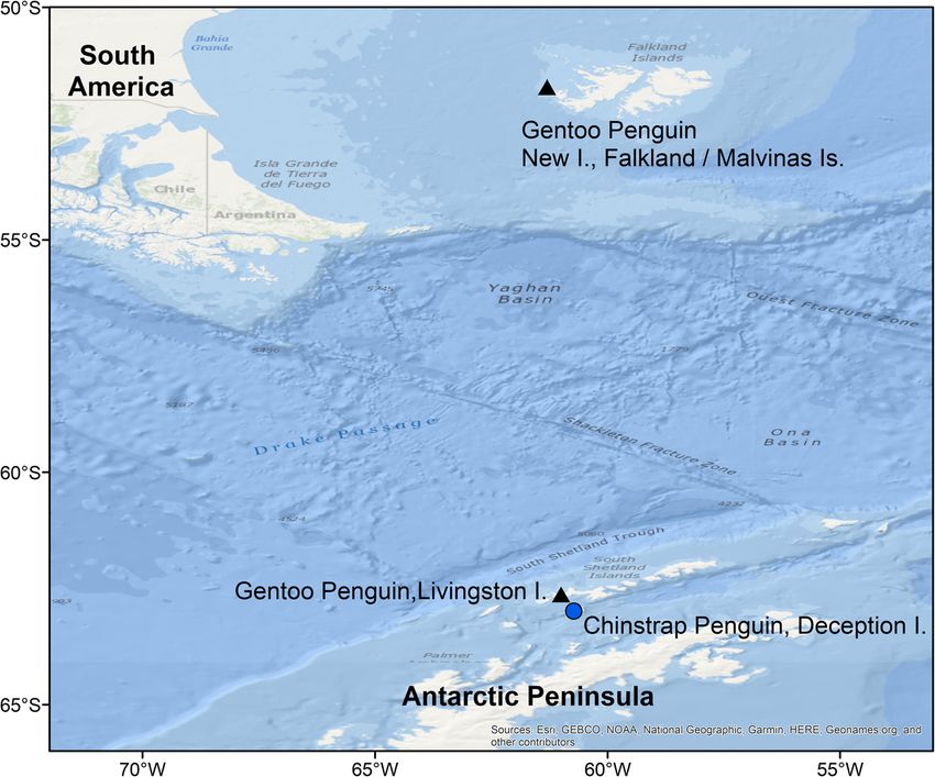
Masello et al. Movement Ecology   (2021) 9:24                                                                    Page 2 of 25

Background                                                    of the energy landscape that result in minimized costs
The current degree of anthropogenic space use, both           and maximised energy gain [19, 21, 23, 25–27].
at sea and land, and climate change make it impera-              In seabirds, variable oceanographic conditions and fluc-
tive to understand animal movement, if meaningful             tuating food availability can affect the costs of moving and
conservation and management measures are to be                energy landscapes capture this variation successfully [21].
taken [1–3]. Animals move to find critical resources          For instance, considering the energetic costs and duration
[4] but increasingly, they have to negotiate habitats         of flights, dive and inter-dive phases, Wilson et al. [23]
that are intensively-used, fragmented, impoverished,          found that imperial cormorants Phalacrocorax atriceps se-
or modified by climate change, which may determine            lected foraging areas that varied greatly in the distance
individual survival and thus, population dynamics and         from the breeding colony and in water depth, but always
persistence [5–7]. Simultaneously, a growing availabil-       indicated minimal energetic cost of movement compared
ity of high-resolution animal tracking technologies has       with other areas in the available landscape. Likewise,
greatly enhanced our ability to describe animal move-         evaluating the daily energy requirements of an individual
ments [4, 8, 9], which in turns guides and refines            using the biophysical properties of bodies (body shape and
conservation and management measures [10, 11].                its heat flux) exposed to specific microclimatic conditions
Moreover, current technologies offer a unique oppor-          (sea surface temperature, SST, air temperature, cloud
tunity to explore pioneering questions in ecology, and        cover, relative humidity and wind speed), Amélineau et al.
to explain in depth the causes and fundamental                [27] found that little auks Alle alle targeted areas with
mechanisms of movement patterns and their signifi-            moderately elevated energy landscapes in winter. In gen-
cance for ecological and evolutionary processes [8, 9,        too penguins Pygoscelis papua (hereafter gentoos), when
12].                                                          considering mass-specific costs of foraging to dive to a
  The first systematic attempts to understand the role of     particular depth plus commuting to a certain distance,
behaviour in the distribution of animals originated from      and energy gained in terms of diving bottom time, the en-
optimal foraging theory [13, 14]. In this context, animals    ergy landscapes around two nearby colonies varied
should exhibit behaviours that maximize energetic effi-       strongly between years. Yet, the birds consistently used
ciency, selecting patches where the gain per unit cost is     the areas of the energy landscape that resulted in lower
high, and the energy expenditure to reach them is mini-       foraging costs. However, for these gentoos the breeding
mized. As movement accounts for such a large propor-          success was low in a year of higher energy expenditure,
tion of animal energy budgets, energetic constraints with     while it was high during a year of lower energy expend-
respect to space use, migration and foraging range are        iture, suggesting the usefulness of energy landscapes to
foreseeable factors [15–17]. Unnecessary movements            understand demographic changes and their consequences
and resulting energy deficits might increase the risk of      for conservation [21].
predation, reduce body condition, increase physiological         We combined information from previous work on the
stress, affect fitness, and since the sum of individual re-   energy landscape in gentoos [21] with novel data on move-
sponses is ultimately reflected at the population-level, be   ment and diet and 1) studied the response of moving ani-
the cause of population declines [12, 18–22]. Animal          mals to different energy landscapes and resources, and 2)
movement has also been investigated in terms of the           compared populations with contrasting population trends.
physical mechanics of motion (biomechanical paradigm),        Gentoos are facing strong environmental change both in
the movement-related decisions made by the individuals        Antarctic and sub-Antarctic regions. The Antarctic Penin-
(cognitive paradigm), and the theories of random walk,        sula is one of the places where current environmental
diffusion, and anomalous diffusion (random paradigm)          change is fastest [28]. In both regions, gentoos are known
[6]. More recently, the paradigm of energy landscape has      to show considerable plasticity in their diet, diving, and for-
opened a new approach to the mechanistic basis of             aging behaviour [29, 30], providing a buffer against changes
spatial ecology and decision-making in wild animals           in prey availability [31]. However, gentoos exhibit strikingly
[12]. The energy landscape paradigm (sensu Wilson             different population trends in sub-Antarctic and Antarctic
et al.) [23] allows the quantification of the variation in    populations. Since 1990, gentoos at the Falkland/Malvinas
the energy costs of the movement through a given envir-       Islands showed a great degree of inter-annual variability in
onment [12], as well as how these costs vary in time and      the number of breeding individuals, which has been related
for different animal populations moving there [21], using     to the Southern Oscillation Index (SOI) and the El Niño
for instance environmentally dependent costs of trans-        Southern Oscillation (ENSO), yet the underlying mecha-
port generated by parameters such as incline, substrate       nisms remain unknown [32]. In contrast, gentoos have been
type, vegetation, current speed, or direction [24]. Re-       increasing at breeding colonies along the Antarctic Penin-
search conducted in organisms as diverse as fish, mam-        sula and expanded southwards since 1979 [33–35]. This
mals, and birds showed that animals will move in areas        positive population trend was understood as gentoos being
Masello et al. Movement Ecology        (2021) 9:24                                                                                      Page 3 of 25

the ‘winners’ among Pygoscelis penguins of the reduction in                 where low energy is required, b) in suboptimal breeding
the sea-ice cover in the region because it positively affects               sites like the Falkland/Malvinas Islands (fluctuating popu-
its winter survival (sea-ice hypothesis) [36]. An alternative               lations) gentoos are forced to forage in more expensive
hypothesis postulated that penguin population dynamics in                   conditions in the poorer years, and c) foraging in areas of
Antarctica were instead controlled through “top-down” fac-                  the energy landscapes that result in minimized energetic
tors such as competition for prey [37], while another related               costs will lead to better individual condition, as shown by
hypothesis suggested a link between penguin population                      physiological parameters such as leucocyte counts. To
trends and changes in the abundance of their main prey,                     understand our results in a wider context, we also investi-
Antarctic krill Euphausia superba [38]. However, it has                     gated the diet and the energy landscape in chinstrap pen-
been shown that sea-ice cover and krill abundance are in-                   guins Pygoscelis antarcticus (hereafter chinstraps), an
terrelated [39, 40]. Even more, other aspects need to be                    Antarctic species with currently declining populations [35,
considered, such as fine-scale spatial heterogeneity in popu-               43, 44]. We tested the hypothesis that d) chinstraps show
lation dynamics observed on the Antarctic Peninsula [41],                   higher energy expenditure than Antarctic gentoos.
intra-specific competition [40], and adaptive shifts in
trophic position [42]. But, regardless of this research, no                 Methods
study has yet considered the cost of foraging. The energy                   Study sites and species
landscape approach could provide a way to better under-                     We collected data on three penguin populations: gentoos
stand the ecological processes involved, as the energetic                   from an Antarctic and a sub-Antarctic breeding site, and
balance between costs and benefits will affect how and                      chinstraps from an Antarctic breeding site. We studied a
which foraging areas are selected or avoided, and the condi-                population of gentoos breeding at a colony located in Devils
tion of the birds which in turn will affect reproductive suc-               Point, Byers Peninsula, Livingston Island, South Shetland
cess and ultimately population dynamics.                                    Islands, maritime Antarctica (hereafter Livingston; 3000
   In our present study we tested the following hypotheses:                 nests; 62°40′S, 61°13′W; Fig. 1) [45]. Byers is characterised
a) in optimal sites (Antarctic Peninsula and islands around                 by a high biological diversity due to relatively mild climatic
it) gentoos forage in sectors of the energy landscapes                      conditions and a large ice-free area in summer [45]. This

 Fig. 1 Overview of the location of the studied gentoo penguin Pygoscelis papua colonies at Devils Point, Byers Peninsula, Livingston Island, South
 Shetland Islands, maritime Antarctica, and New Island, Falkland/Malvinas Islands, and the chinstrap penguin Pygoscelis antarcticus colony at
 Vapour Col rookery, Deception Island, South Shetland Islands, maritime Antarctica
Masello et al. Movement Ecology            (2021) 9:24                                                                                               Page 4 of 25

breeding population is located in an optimal breeding site,                          species see Table 1. We captured the birds mostly by
as gentoos are increasing in numbers in this location in the                         hand, in the nests, with the occasional help of a hook at-
last decades [45], following the population increase and                             tached to a rod [21] or a long-handle net [47]. To pro-
area expansion in this region [33, 41]. We furthermore in-                           tect them from predators, we also captured the chicks
vestigated energy landscapes of chinstraps at Vapour Col                             during the handling of the adult. We kept handling time
rookery on the west side of Deception Island, South Shet-                            mostly below 15 min and always below 20 min. We took
land Islands (hereafter Deception; 20,000 breeding pairs;                            extreme care to minimize stress to the captured birds,
63° 00′S, 62°40′W; Fig. 1) [43], a species declining on the                          covering the head during handling in order to minimize
Antarctic Peninsula [41, 44]. We further studied the for-                            the risk of adults regurgitating. During this procedure
aging strategies and mechanism of gentoos of a fluctuating                           none of the birds regurgitated. We attached the loggers
population, New Island in the Falkland/Malvinas Islands                              on the adult penguin with adhesive Tesa® 4651 tape [21].
(hereafter New Island) [21, 32]. On New Island, we investi-                          The loggers used (GPS-TD: 75 to 145 g and Axy-2: 19 g;
gated two breeding colonies: one located at the North End                            Axy-Trek: 60 g) represented a maximum of a 3% of the
(around 5000 breeding pairs; 51° 41.402′ S 61° 15.003′ W),                           adult gentoo body mass (mean for Livingston 5212.8 ±
and one at the South End (around 2000 breeding pairs 51°                             478.2 g, n = 25) or 4% of the adult chinstrap body mass
44.677′ S 61°17.683′ W) [46]. The data previously obtained                           (mean for Deception 3743.5 ± 425.4 g, n = 20), and had a
at New Island [21], as well as samples analysed in current                           shape that matched the body contour to reduce drag
study, are used for the comparisons between optimal and                              [48]. In a previous study [49], we showed that handling
suboptimal breeding sites.                                                           and short-term logger attachments like the ones in this
                                                                                     study showed limited effect on the behaviour and physi-
Instrumentation and fieldwork procedures                                             ology of the birds. After the deployment procedure and
We simultaneously deployed a combination of GPS-                                     immediately before the release of the adult bird, we
temperature-depth (GPS-TD; earth&OCEAN Technolo-                                     returned the chicks to the nest, and released the adults
gies, Kiel) and micro tri-axial accelerometer loggers                                some 20 m from their nests. All birds returned to their
(Axy-2; Technosmart Europe, Rome, Italy) or Axy-Trek                                 nests and attended their chicks shortly after being re-
loggers only (including GPS, accelerometer, and both                                 leased. The loggers recorded detailed position (longitude,
pressure and temperature sensors), on the penguins dur-                              latitude; sampling interval: 5 min), dive depth (reso-
ing chick guard. For sample sizes per study site and                                 lution: 3.5 cm; sampling interval: 1 s), time of day and

Table 1 Parameters of foraging trips used for the calculations of energy landscapes
                               Gentoo                                                                                                          Chinstrap
                               Dec 2013              Dec 2014                                     Dec 2016                                     Jan 2017
                               New I., South         New I., South          New I., North         Livingston I.                                Deception I.
                                                                                                  Short trips            Long trips
Individuals tagged             16                    8                      8                     26                                           18
Number of complete trips       13                    4                      6                     26                     19                    18
                                      b                     a, b                 a                      c                     a
Median trip length [km]        125.6                 88.7                   59.1 (52.2–61.7)      27.1 (19.9–33.4)       66.6 (59.2–71.0)      37.7 d (21.7–49.5)
                               (87.4–161.8)          (40.8–144.7)
Kruskal-Wallis                 χ2 = 72.1, df = 5, P < 0.001
Median maximum distance 66.9 b (63.2–75.6)           47.7 a, b              29.6 a, b (19.8–45.1) 11 c (8.6–13.4)        25.7 a (23.5–32.1)    15.5 d (8.7–20.2)
from colony [km]                                     (23.7–75.6)
Kruskal-Wallis                 χ2 = 75.3, df = 5, P < 0.001
Median trip duration [min]     1727.3 a              1579.6 a               1129 a                503.4 b                1049 a                595.5 b
                               (1062.4–2432.6)       (765.2–2508.0)         (850.3–1538.9)        (373.2–641.7)          (866.1–1182)          (371.2–641.6)
Kruskal-Wallis                 χ2 = 67, df = 5, P < 0.001
Median start time of           03:41:46 c          16:49:26 a, b       09:15:50 a, b, c    14:52:48 a          09:31:41 b, c       15:38:53 a
foraging (local time)          (03:05:46–14:18:14) (11:47:02–18:25:55) (03:14:24–17:13:55) (10:10:34–17:45:36) (03:10:05–16:00:29) (07:16:19–18:34:34)
Kruskal-Wallis                 χ2 = 17.3 df = 5, P < 0.001
The data correspond to gentoo penguins Pygoscelis papua breeding at New Island (Falkland/Malvinas Islands), during chick guard (December) in 2013 and 2014,
gentoo penguins breeding at Devils Point, Byers Peninsula, Livingston Island, South Shetland Islands, Antarctica, during chick guard (December 2016), and
chinstrap penguins Pygoscelis antarcticus breeding at Vapour Col rookery, Deception Island, South Shetland Islands, Antarctica, during chick guard (January 2017).
See also Figs. S7 and S8 in Additional file 1
Note: Sample sizes vary with respect to deployments, as not all parameters could be calculated for all individuals, mainly due to some batteries running out
before the finalization of an ongoing trip. Statistically significant values are marked bold. Dunn’s homogenous subgroups are indicated in superscript
similar letters
Masello et al. Movement Ecology (2021) 9:24 Page 5 of 25
acceleration (sampling interval: 50 Hz) measured in three distance between the furthest point of the recorded trip
directions (x, y, z, i.e. surge, sway, heave) [21]. The de- and the geographical coordinates of the departure col-
vices operated for three to 9 days and had to be recov- ony, determined by GPS [21, 51]. We calculated trip
ered to access recorded data. We recaptured the birds in duration as the time difference between the onset of the
their nests. After device removal, we measured flipper first dive performed after leaving and the end of the last
and bill length, bill depth, and body mass, and collected dive event before arriving back at the colony. For the
blood samples (200 μl) from the foot (Antarctica) or the identification of foraging dives, we used purpose-written
brachial (New Island) vein, and four small feathers from scripts in Matlab (The Mathworks Inc., Nattick, USA)
the lower back of the adults. Blood and feather samples and in IGOR Pro 6.3. (WaveMetrics, Lake Oswego,
were used for the study of stable isotopes (see Stable iso- USA). Following Mattern et al. [55] and in order to
tope analysis of the diet below) and molecular sexing avoid depth measurement inaccuracy in the upper part
(following standard methods) [50]. As in previous stud- of the water column, we accepted dive events only when
ies [21, 51], we detected no adverse effects related to depths > 3 m were reached. We defined the bottom
blood sampling. One drop of blood was smeared and air phase as a period of the dive between a steady pressure
dried on a glass slide directly after sampling, and fixed increase at the beginning of the dive (i.e. descent) and
with absolute methanol and stained with Giemsa dye the continuous pressure decrease indicating the pen-
later in the laboratory [52]. Blood smears were used for guins’ ascent back to the surface [55, 56]. We also calcu-
differential leucocyte counts (see Condition parameters lated the maximum depth (in m) reached during a dive
below). Additionally, we collected fresh scat samples op- event (hereafter event maximum depth), and the number
portunistically during the handling of the birds, as well of dive events during a particular foraging trip. For each
as from randomly located ice or rock substrates around dive, we calculated a geographical position either by
the penguin colonies, immediately after defecation. To using the half way point between GPS fixes recorded im-
avoid external contamination, we took special care to mediately before and after the dive, or by calculating the
collect the central part of the scat and not the part that relative position along a linear interpolated line between
was in direct contact with the substrates. We kept scat the last fix obtained and before the first fix after the dive
samples cool with ice packs during fieldwork, froze them occurred based on the time the dive occurred relative to
once back at the field station, and transported frozen these fixes. Because in previous studies we found that
until processed in the laboratory. gentoos at New Island take both benthic and pelagic
prey [21, 51], we split the foraging dives performed by
Spatial and temporal data the individuals in benthic and pelagic ones for further
We downloaded tri-axial acceleration data and GPS files, analyses. We did this by calculating the index of benthic
comprising location (WGS84) and time, and a separate diving behaviour developed by Tremblay & Cherel [56].
file containing dive depth and water temperature data This method assumes that benthic divers dive serially to
from the recovered loggers (Table 1). Sample sizes a specific depth, and therefore consecutive dives reach
(Table 1) varied due to logger failures that prevented to the same depth zone. These are called intra-depth zone
produce complete data sets for some individuals. Fail- (IDZ) dives [56]. As in previous studies, we defined the
ures corresponded to 1) loggers damaged by salt water IDZ as the depth ± 10% of the maximum depth reached
reaching the electronic components, 2) broken GPS an- by the preceding dive [21]. During the current study,
tennas, and 3) batteries that were unexpectedly depleted. gentoos performed a varying proportion of benthic and
As in previous studies [21, 51], we defined foraging trips pelagic dives, which we considered in following analyses.
from the time when the birds departed from the colony As the inspection of histograms showed that the data for
to the sea until returning to the colony. To obtain bathy- pelagic dives was left shifted, we used the median dive
metric data for Antarctica, we used the International depth per colony per year for further calculations involv-
Bathymetric Chart of the Southern Ocean (IBCSO) [53], ing pelagic dives (Table 2; Additional file 1, Figs. S1, S2).
while for the Falkland/Malvinas Islands, we used ba- We show the distribution of benthic and pelagic dives in
thymetry data from the global sea floor topography from Figs. S3, S4 (Additional file 1). We also calculated the
satellite altimetry and ship depth soundings (Global median number of dives performed during the foraging
Topography) [21, 54]. We used QGIS 3.4 (QGIS Devel- trips (Table 2). In previous studies [21, 51], we found
opment Team) to plot and analyse positional data of the that gentoos showed no sexual differences in foraging
trips performed by the birds. We calculated trip length behaviour parameters. Gentoos from Livingston showed
as the total cumulative linear distance between all pos- also no sexual differences in foraging (Additional file 1,
itional fixes along the foraging trip, outside of the col- Figs. S5). Therefore, in this study, we pooled the data of
ony. For each trip, we determined the maximum males and females. We used the nonparametric fixed
distance from the colony as the linear grand circle kernel density estimator to determine the 50% (coreMasello et al. Movement Ecology (2021) 9:24 Page 6 of 25
Table 2. Dive parameters used for the calculations of energy landscapes
Gentoo Chinstrap
Dec 2013 Dec 2014 Dec 2016 Jan 2017
New I., South New I., South New I., North Livingston I. Deception I.
Short trip Long trip
Maximum dive depth [m] 188.3 178.2 156.3 79.9 109.9 111.9
Median dive depth of pelagic dives [m] 15.8 e (3–185.9) 12.7 a,b (3–176.6) 21.1 c (3–156.5) 14.9 a (3–79.9) 15.4 b 12.3 d
(3–109.9) (3–105.3)
Kruskal-Wallis χ2 = 322.3 df = 5, P < 0.001
Median proportion of benthic dives 24 (19–30) 46 (33–66) 63 (50–67) 48 (39–53) 26 (24–39) 31 (24–43)
(pBD) [%]
Median proportion of pelagic 76 d (70–81) 54 a,b (34–67) 37 a (33–50) 52 a (47–61) 74 c,d (61–76) 69 b,c (57–76)
dives (pPD) [%]
Kruskal-Wallis χ2 = 24.6 df = 5, P < 0.001
Median number of dives per 283 a, c 291 a, b, c
(193–471) 298 a, b, c (241–331) 215 a (156–268) 402 b (299–744) 369 c
foraging trip (MND) (202–337) (205–497)
Kruskal-Wallis χ2 = 19.6 df = 5, P = 0.002
Median dive duration (DD), 156 a (142–177) 155 a (150–199) 176 a (157–202) 81 b
(71–96) 90 b (82–95) 70 c (60–85)
benthic dives [s]
Kruskal-Wallis χ2 = 61.2 df = 5, P < 0.001
Median dive duration (DD), 103 a (92–119) 123 a, b
(117–125) 130 a (127–138) 67 c (63–73) 83 b (72–88) 55 d (51–69)
pelagic dives [s]
Kruskal-Wallis χ2 = 69.8 df = 5, P < 0.001
Minimum benthic bottom 2 3 2 2 3 2
time (mBBT) [s]
Parameters correspond to gentoo penguins Pygoscelis papua breeding at New Island (Falkland/Malvinas Islands), during chick guard (December) in 2013 and 2014,
gentoo penguins breeding at Devils Point, Byers Peninsula, Livingston Island, South Shetland Islands, Antarctica, during chick guard (December 2016), and
chinstrap penguins Pygoscelis antarcticus breeding at Vapour Col rookery, Deception Island, South Shetland Islands, Antarctica, during chick guard (January 2017).
Only the first foraging trip of each individual was included in the calculations in order to avoid individuals with more than one trip having more weight in the
analyses. See also Figs. S1 to S4 in Additional file 1
Notes: Statistically significant values are marked bold. Dunn’s homogenous subgroups are indicated in superscript similar letters
area) and 95% (home range) density contour areas (esti- by the studied penguins. With the data obtained from
mated foraging range) [57, 58] of dive locations (i.e. GPS the deployed penguins, we calculated the energy land-
position at the onset of a dive event). Kernel densities in- scapes for a grid of the marine area around the islands
dicate the places in a foraging trip where birds spent with the breeding colonies for which detailed bathymet-
most of their time [57]. For these calculations we used ric data was available. We carried out the quantification
both the Geospatial Modelling Environment (Spatial as in Masello et al. [21], to allow comparisons, and
Ecology LLC, http://www.spatialecology.com/gme/) and followed a series of steps.
QGIS 3.4 (QGIS Development Team).
As for trip and dive parameters (Tables 1 and 2) nor-
mality and equality of variance were not satisfied (P < Step 1, calculation of the overall dynamic body acceleration
0.05; Additional file 1, Figs. S7, S8), we investigated dif- Since the major variable factor in modulating energy ex-
ferences using the Kruskal–Wallis test (one-way penditure in vertebrates is movement and measurements
ANOVA on ranks) and Dunn’s homogenous subgroups of body acceleration correlate with energy expenditure
implemented in the R package dunn.test v1.3.5 (R Devel- (reviewed in [60]), we used tri-axial acceleration data to
opment Core Team, https://www.r-project.org/) [59]. calculate the Overall Dynamic Body Acceleration
(ODBA) for all first foraging trips of the deployed indi-
Calculation of energy viduals. ODBA is a linear proxy for metabolic energy
Using tri-axial acceleration data (Additional file 1, Fig. that can be further converted into energy expenditure
S6), we quantified energy landscapes as the mass-specific [16, 23, 60, 61] but see also [62]. As in previous studies
total cost of foraging, including diving and commuting, [21, 51], only the first foraging trip of each individual
relative to the bottom time, which we selected as a proxy was included in the calculations to avoid individuals with
of energy gained from feeding. We considered the differ- more than one trip having more weight in the analyses,
ent proportion of benthic and pelagic dives carried out and to allow comparisons.Masello et al. Movement Ecology (2021) 9:24 Page 7 of 25
We calculated ODBA (expressed as gravitational force Step 3, calculation of the cost of travelling
g) using a purpose-written script for IGOR Pro 6.3 In seabirds like penguins, which cover large distances to
(WaveMetrics, Lake Oswego, USA) and the sum of the reach their foraging grounds, it is important to include
absolute values of dynamic acceleration from each of the the energy cost of travelling for any calculations of the
three spatial axes (i.e. surge, sway, and heave; sampling cost of foraging. In previous work [21, 51], we found that
interval: 50 Hz) after subtracting the static acceleration gentoos performed foraging trips of up to 282 km, while
(= smoothed acceleration; smoothing window: 1 s) from up to 139 km were reported for chinstraps [67]. We first
the raw acceleration values following Wilson et al. [23]: calculated the distance between each point in the marine
area grid around the islands with the penguin breeding
colonies (see Step 2) with the Geospatial Modelling En-
ODBA ¼ jAxj þ jAyj þ jAzj ð1Þ
vironment and QGIS 3.4. Using this distance and the
mean swimming speed previously calculated for gentoos
Ax, Ay and Az are the derived dynamic accelerations at (2.3 m s− 1) [68], we were able to calculate the travel time
any point in time corresponding to the three orthogonal needed for the birds to reach each of the 8130 locations
axes of the Axy-2 or the Axy-Trek acceleration loggers around the islands for which bathymetric data were
deployed on the penguins. available. The travel time (TT, in s), and their minimum
metabolic cost of transportation previously determined
in a swim canal and at sea (16.1 W kg− 1) [68, 69],
Step 2, calculation of benthic and pelagic ODBAs allowed us subsequently to calculate the minimum cost
In diving seabirds, power costs during dive vary with the of travelling (CT, in J kg− 1) to each location in the grid
depth exploited [63, 64], and penguins take both benthic used to construct the energy landscapes:
and pelagic prey [21, 51, 65]. For both reasons, we split
the foraging dives performed by the individuals in ben- CT ¼ TT16:1 W kg‐1 ð2Þ
thic and pelagic ones, calculated the corresponding ben-
thic and pelagic ODBAs, and interpolated them for the
available bathymetric data points around the breeding Step 4, calculation of the cost of a dive
colonies. To quantify the cost of a dive, including the cost of the
For this step, we first investigated the relationship be- pursuit of prey during a dive, we first had to measure its
tween the ODBAs calculated in Step 1 and penguins’ energy expenditure. The rate of oxygen consumption Vo
maximum dive depth. We found that the sum of ODBA (in ml min− 1) is an indirect measure of energy expend-
during the dives carried out by the penguins was related iture commonly used under laboratory conditions (for
to the maximum dive depth they reached (0.70 < R2 < examples see [60]) but difficult, if not impossible, to use
0.78; see also Additional file 1, Figs. S9-S12). However, in diving seabirds like penguins. An alternative tech-
using a general additive model implemented in the R nique for free-ranging animals is to use ODBAs as a cali-
package GAM [66] we found that this relationship dif- brated proxy for the rate of oxygen consumption Vo [61,
fered between benthic and pelagic dives both for gentoos 70], which can be used to calculate the total energy ex-
and chinstraps (Additional file 1, Table S1). Thus, we penditure during a dive.
determined the regressions with the best fit for the dif- Previous research demonstrated a linear relationship
ferent dive types, benthic and pelagic, in SigmaPlot 10 between ODBA and energy expenditure in all species ex-
(Systat Software, San Jose, USA). We provide the regres- amined to date (summarised in [23]; but see [62, 71]).
sion descriptions and corresponding parameters in Table Following the method developed by Wilson et al. [70]
S2 (Additional file 1). We used the regressions between and tested by Halsey et al. [61] in several species, we first
the sum of ODBA during the dive of the deployed pen- calculated Vo:
guins and the maximum dive depth (Additional file 1,
Table S2), together with the bathymetric data points Vo ¼ 9:16 þ ODBA16:58ðfor gentoosÞor Vo
from IBCSO [53] to calculate benthic ODBAs for a grid ¼ 7:15 þ ODBA12:04ðfor chinstrapsÞ ð3Þ
of the marine area around the penguin colonies (ap-
proximately 100 km around the islands; n = 8130; grid We calculated the intercept and slope in (3) also fol-
spatial resolution as in IBCSO: 500 × 500 m, based on a lowing Halsey et al. [61]. These authors found that the
polar stereographic projection) separately for each spe- intercept and the slope for the relationship between
cies. To calculate the pelagic ODBA, we used the regres- ODBA and Vo (in ml * min− 1) in all species studied
sions (Additional file 1, Table S2) and the median dive could be calculated as: intercept, y = 2.75 * BM0.73 (R2 =
depth (Table 2), as pelagic dive depth data were not nor- 0.89), slope, y = 3.52 * BM0.94 (R2 = 0.94), with BM being
mally distributed but left-shifted. the mean adult body mass in kg.Masello et al. Movement Ecology (2021) 9:24 Page 8 of 25
The uptake of 1 l of oxygen can be converted into an Step 6, integrating the cost of diving and commuting
energy expenditure estimate of approximately 20 kJ [72], The parameters calculated in Step 5, together with previ-
such that 1 ml O2/min equals 0.333 J s− 1. Finally, to de- ous calculations of CT (Step 4), allowed us to calculate
rive the energy expenditure (in J kg− 1 s− 1) relative to the the total cost of foraging (TCF, in J kg− 1) as:
body mass of the penguins (also called mass-specific
power, MP, e.g. [21, 23]), we divided the energy expend-
TCF ¼ MPMND benthic þ MPMND pelagic þ CT2 ð7Þ
iture by the mean weight of the penguins (gentoos: 5.2
kg; chinstraps: 3.7 kg; individuals measured in this
study): CT is multiplied by two to account for the return to
the breeding colony.
MP ¼ Vo 0:333=BM ð4Þ
Step 7, calculating the energy gained during foraging
Previous studies on several penguin species have
The equation in (4) allowed us to calculate the MP
found a positive relationship between bottom times
separately for benthic dives (MPbenthic, using benthic
(duration in s of bottom dive phase) and prey cap-
ODBA from Step 2 in Eq. 3) and pelagic dives (MPpelagic,
ture: Southern rockhoppers Eudyptes chrysocome have
using pelagic ODBA from Step 2 in Eq. 3) for each point
been found to maximise bottom time, which in this
in the grid around the islands used to construct the en-
species equalled feeding time [56]; chinstraps showed
ergy landscapes.
a positive linear relationship between bottom time
and the number of underwater beak-opening events
Step 5, integrating the cost of the actual number of dives
during dives, and that most (86%, n = 4910 events) of
performed
beak-openings occurred during the bottom times [73];
Subsequently, we calculated the MP for each point of
king Aptenodytes patagonicus and Adélie Pygoscelis
the marine area’s grid around the islands with the stud-
adeliae penguins ingested prey mostly during the bot-
ied breeding colonies for the number of benthic and pe-
tom phase of diving [74]; and little penguin Eudyp-
lagic dives carried out by the penguins. In the case of
tula minor showed longer bottom times associated
chinstraps, we used the median number of dives per for-
with dives where prey was captured [75]. Thus, sev-
aging trip (MND; Table 2) together with the mean dive
eral studies have successfully used bottom time as a
duration (DD, duration in s of the dive event; Table 2),
proxy for prey acquisition and energy gained both in
assuming a gradient of bottom depths from 3 m (mini-
penguins [21, 76] and other seabirds [77]. To build
mum depth consider a dive, see the justification in
energy landscapes that also include the energy gained
Spatial and temporal data) to the maximum depth (=
during foraging, we calculated bottom times and
bathymetric depth) for benthic dives, and a gradient of
minimum benthic bottom times (mBBT; Table 2).
bottom depths from 3 m to median dive depth for pela-
The bottom times from the first foraging trip of each
gic dives as follows:
individual showed a relationship with maximum dive
depth. This relationship also differed between benthic
MPMND benthic ¼ DDbenthic MPbenthicð3 m depthÞ þ MPbenthic MND=2pBD and pelagic dives (GAM; Additional file 1, Table S4).
ð5Þ Again here, we determined the regressions with the
best fit for the different dive types in SigmaPlot 10.0
(Additional file 1, Table S5; Figs. S14-S17). The re-
MPMNDpelagic ¼ DDpelagic MPpelagicð3 m depthÞ þ MPpelagic MND=2pPD
gressions between bottom time and maximum dive
ð6Þ depth (Additional file 1, Table S5), allowed us to cal-
culate the sum of benthic bottom time (BBT) for
where pBD is the mean proportion of benthic dives and each point of the grid of the marine area around the
pPD the mean proportion of pelagic dives (Table 2), in- islands with the studied breeding colonies used to
cluded accounting for the proportion of benthic and pe- construct the energy landscapes, separately for each
lagic dive in a single foraging trip. species. For pelagic bottom times (PBT), we used the
In the case of gentoos, which in addition to pelagic corresponding regressions (Additional file 1, Table S5)
and benthic dives performed short and long trips and and the median dive depth per species (Table 2). To
showed a relationship between the number of dives and calculate the total bottom time (TBT, in s), we took
the maximum distance from the colony during a for- into account that the birds start diving close to the
aging trip (Additional file 1, Fig. S13), we used the re- colony (as also found in [21, 51]) and increase dive
gression in Table S3 (Additional file 1) to compute depth while gaining distance. A mean is calculated
MND. and the mean multiplied per MND:Masello et al. Movement Ecology (2021) 9:24 Page 9 of 25
TBT ¼ ðmBBT þ BBTÞ=2MNDpBD þ PBTMNDpPD ð8Þ to reference sequences in the National Center for Bio-
technology Information (NCBI) GenBank nucleotide
We also included pBD and pPD here to account for database, using a cut-off of 90% minimum sequence
the proportion of benthic and pelagic dive in a single identity and a maximum e-value of 0.00001. For the bio-
foraging trip. informatics analyses of the samples from Antarctica, we
carried out all those analyses using a custom workflow
Step 8, construction of the energy landscapes in GALAXY (https://www.computational.bio.uni-giessen.
Finally, dividing TCF (7) by TBT (8), we were able to de/galaxy) [84]. As next step, we manually discarded
calculate the total relative cost (TRC, in J kg− 1 s− 1), MOTUs that corresponded to regular fieldwork contam-
which is the mass-specific total cost of foraging (diving inants in faecal samples, such as bacteria, soil fungi, hu-
plus commuting) relative to the energy gained. Using man or predator DNA. We based taxonomic assignment
TRC values calculated for the grid of the marine area on the percentage similarity of the query and the refer-
around the islands with the breeding colonies, we con- ence sequences. Since short fragments are less likely to
structed the energy landscape by applying the inverse contain reliable taxonomic information, we only retained
distance weighted (IDW) interpolation in to the result- sequences with a minimum length of 190 bp and a
ing data grid. As in our previous study [21], the IDW BLASTn assignment match greater than 98% [85, 86].
interpolation was chosen as 1) a large set of sample We assigned MOTUs to species-level in cases when all
values was available, and 2) the sample data points rep- retained hits of a MOTU with the same quality criteria
resented the minimum and maximum values in our sur- (sequence identity, sequence length, e-value) corre-
face [78]. In brief, the energy landscapes here presented sponded to the same species, if not we assigned the
are based on the bathymetry of the area and the total MOTU to the lowest shared taxonomic level, e.g. genus
cost of foraging (diving plus commuting) relative to the or family, as in Kleinschmidt et al. [87]. We performed
bottom time (= energy gained, in J kg− 1 s− 1), and take further filter steps to avoid contamination/false positives
into account the different proportion of benthic and pe- and to obtain reliable data [88] as follows: we accepted
lagic dives carried out by the penguins. MOTUs in a sample only if they contained a minimum
of 10 sequences or accounted for > 1% of the maximum
Molecular analysis of the diet total of hits. Additionally, we also discarded taxa with
We collected a total of 247 faecal samples from gentoos very distant or ecologically irrelevant distribution ranges
from the colony at Livingston, chinstraps from the col- (e.g. deserts). Negative controls were included and did
ony at Deception, two colonies at New Island, and po- not show any contaminations. For each taxonomical
tential prey samples to obtain detailed information on level found, we calculated the frequency of occurrence
diet composition (Additional file 1, Tables S6 and S7). (FO) [89]. To visualize differences in diet compositions
Details on deoxyribonucleic acid (DNA) extraction, for the penguin species and for adults and chicks, we
primers used, polymerase chain reaction (PCR) amplifi- performed non-metric multidimensional scaling
cations, library preparations, and next generation se- (NMDS) with the function metaMDS in the R package
quencing (NGS) are provided in the Additional File 1 VEGAN [90]. NMDS uses rank orders to collapse infor-
(Table S8 and Additional Methods). mation from multiple dimensions into usually two-
We used the raw Illumina sequence data to produce a dimensions to facilitate visualization and interpretation,
list of molecular operational taxonomic units (MOTUs). and is generally considered as the most robust uncon-
Bioinformatics analyses included the following steps: strained ordination method in community ecology [91,
assessing sequence quality with FASTQC (http://www. 92]. The function metaMDS allowed us to investigate
bioinformatics.babraham.ac.uk/projects/fastqc), adapter the agreement between the two-dimension configuration
and quality trimming of the paired-end reads with and the original configuration through a stress param-
TRIMMOMATIC (minimum quality score of 20 over a eter. If the stress is < 0.05 the agreement is excellent, <
sliding window of 4 bp) [79], merging of the overlapping 0.1 is very good, < 0.2 provides a good representation. In
paired-end read pairs using FLASH [80], transforming our models the stress was always < 0.04 (excellent). We
sequence files to FASTA with the FASTX-Toolkit performed permutational multivariate analysis of vari-
(http://hannonlab.cshl.edu/fastx_toolkit/), and extracting ance using distance matrices (PERMANOVA) with the
amplicons in MOTHUR [81]. We used USEARCH [82] function adonis and checked for the multivariate homo-
to remove identical replicates (dereplicate; derep_full- geneity of group dispersions (variances) with the func-
length), to detect and to remove chimeric sequences tion betadisper. We also used the functions ordihull and
(uchime_denovo) and to cluster sequences into molecu- ordiellipse to add convex hulls and ellipses to the NMDS
lar operational taxonomic units (MOTUs). Using the plots and improve visualization. To compare the diet
BLASTn algorithm [83] we matched MOTU sequences composition for a certain number of sampledMasello et al. Movement Ecology (2021) 9:24 Page 10 of 25
individuals, we additionally used species accumulation Condition parameters
curves (SAC) with the function specaccum in the R The ratio of two types of leucocytes, the heterophils and
package VEGAN [90]. lymphocytes (H/L ratio), has been successfully used as
an indicator of physiological status and effort (high ra-
tios = high stress) [98, 99]. Following Merino et al. [100],
Stable isotope analysis of the diet differential leucocyte counts were carried out with a
We analysed carbon (δ13C) and nitrogen (δ15N) stable light microscope (× 1000) in parts of the blood smears
isotope ratios of red blood cells. Stable isotope ratios where erythrocytes had separated in a monolayer. The
allowed us to compare the diet the penguins fed during samples were crossed from down to up to minimize dif-
the study period, as red blood cells have a half-life of ca. ferences in the thickness of the blood smear. Leucocytes
30 days [93]. We carried out carbon and nitrogen isotope were counted following Dein [101] and Hawkey and
analyses on 0.65–0.75 mg sample aliquots, weighed into Dennett [102]. A total of 100 leucocytes were counted in
tin cups. Subsequently, we determined carbon and nitro- each smear, thus obtaining percentages of the different
gen isotope ratios by a mass spectrometer (Delta V Plus of leucocyte types and the H/L ratio.
with a Conflo IV interface, Thermo Scientific, Bremen,
Germany) coupled to an elemental analyser (Flash 2000, Additional data
Thermo Scientific, Milan, Italy) at the LIENSs laboratory We obtained the location of other gentoo and chinstrap
from the University of La Rochelle, France. Replicate penguin colonies in the South Shetland Islands, Antarc-
measurements of internal laboratory standards indicated tica, from the Mapping Application for Penguin Popula-
measurement errors < 0.15 ‰ for δ13C and δ15N. Re- tions and Projected Dynamics [103] and Naveen et al.
sults are expressed in the δ unit notation as deviations [104], and the locations of Fur Seal Arctocephalus
from standards (Vienna Pee Dee Belemnite for δ13C and gazella colonies from Hucke-Gaete et al. [105]. We
N2 in air for δ15N) following the formula: δ13C or downloaded Antarctic Krill Euphausia superba abun-
δ15N = [(Rsample/Rstandard) - 1] × 103, where R is 13C/12C dance data for the sector between 60 and 65°S and 55–
or 15N/14N, respectively. Internal laboratory standards 65°W from KRILLBASE [106], and obtained Antarctic
(acetanilide) were used to check accuracy. Measurement Krill catches for the Commission for the Conservation
errors were < 0.15‰ for both δ13C and δ15N. of Antarctic Marine Living Resources (CCAMLR) Area
We compared the isotopic niches of penguins using 48 from the Krill Fishery Report 2018 [107]. Breeding
SIAR (Stable Isotope Analyses in R) [94] and SIBER success data corresponds to the number of chicks per
(Stable Isotope Bayesian Ellipses in R) [95]. The loca- nest at the crèche, and was obtained as part of ongoing
tion of the centroid (mean δ13C, mean δ15N) indicates projects (Vapour Col rookery, Deception, [43, 108] and
where the niche is centred in isotope space. We used AB unpubl. Data; New Island, [21] and PQ unpubl. Data;
a Bayesian approach based on multivariate ellipse ) or from studies in the West Antarctic Peninsula region
metrics to calculate the Bayesian standard ellipse area that followed the same methodology we used (Peter-
(SEAb), which represents the core isotope niche width mann Island, [109]; Goudier Island, [110]). Other avail-
as described by Jackson et al. [95]. In addition, we able studies for the region were excluded, as their
calculated standard ellipse areas based on Maximum methodology clearly differed from the one here used.
Likelihood (SEA), and corrected for sample size Due to logistics limitations of our expedition to Antarc-
(SEAc). We depicted ellipses using the draw.ellipse tica, breeding success data at Livingston, could not be
command of the R package PLOTRIX [96], with the gathered.
lengths of the two semi-major axes and the angle of
the semi-major axis of the ellipse with the x-axis as Results
parameters. To describe the spread of the data points, Foraging trips and dive parameters
we calculated parameters as described by Layman In Antarctica, both gentoos and chinstraps foraged rela-
et al. [97]. As proxies of intra-population trophic di- tively close to their own colonies (Fig. 2), using the col-
versity, we also calculated the mean distance to cen- ony’s ‘hinterland’ (sensu Cairns [111]) and hence,
troid (CD) and the mean nearest-neighbour distance avoided areas closer to the neighbouring colonies and
(NND). We give information on the trophic length of those from potential predators (Additional file 1, Fig.
the community as the δ15N range (NR), and provide S18), and performed trips with the usual loop shape (Fig.
an estimate of the diversity of basal resources by the 2). Gentoos from Livingston performed short (19.9–33.4
δ13C range (CR). We split the data from gentoos into km) and long (59.2–71 km) trips, which strongly differed
male and female adults, and first and second hatched in both length (median, short trip: 27.1 km, long trips
chicks but, due to low samples size, we were not able 66.6 km; Table 1, Fig. 2a), and in the extent of the core
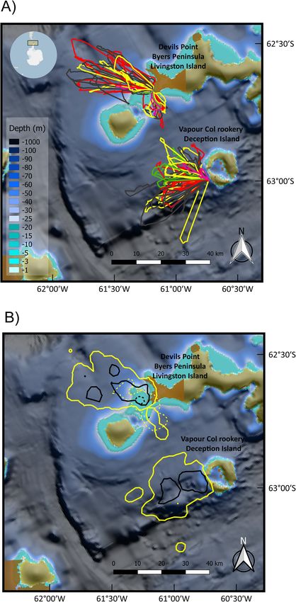
to split chinstrap data. areas and home ranges used (Fig. 2b; Additional file 1,Masello et al. Movement Ecology (2021) 9:24 Page 11 of 25 Fig. 2 Foraging trips (a) and kernel density distribution of dive locations (b). Data from gentoo penguins Pygoscelis papua breeding at Devils Point, Byers Peninsula, Livingston Island, South Shetland Islands during chick guard (December 2016), and chinstrap penguins Pygoscelis antarcticus breeding at Vapour Col rookery, Deception Island, South Shetland Islands, during chick guard (January 2017). Trip lines are colour coded. Dark grey: first recorded trips, red: second trips; yellow: third trips, green: fourth trips; pink: fifth trips. The 50% core areas are denoted by black lines, while 95% home ranges by yellow lines. Kernels from gentoo penguins are further coded for short (dashed lines) and long trips (solid lines). Kernels from chinstrap penguins are denoted by solid lines only, as no distinction between short and long trips could be found. Depth (in m) is based on data from the International Bathymetric Chart of the Southern Ocean (IBCSO) [53] Fig. S19). The short trips carried out by gentoos from but substantially different than the much longer trips Livingston were shorter than any of the trips performed performed by New Island birds during 2013 (median, by New Island birds (minimum trip: 40.8 km), while the 125.6 km; Table 1). The trips performed by chinstraps long trips were similar to those carried out by New Is- from Deception (median 37.7 km) were intermediate be- land birds in 2014 (median, South: 88.7, North: 59.1 km) tween the long and short trips from gentoos from
Masello et al. Movement Ecology (2021) 9:24 Page 12 of 25
Livingston (Table 1). Other related trip parameters are (up to 137.6 J kg− 1 s− 1) or those from New Island South
provided in Table 1. 2013 and 2014 (up to 232) but similar to those from New
In Antarctica, the maximum dive depth was recorded Island North 2014 (up to 151.9) (pairwise Kruskal-Wallis
in chinstraps (111.9 m, Table 2). However, maximum rank sum test in Additional file 1, Table S9; all P-values <
dive depth achieved by both gentoos (109.9 m) and chin- 0.001 except for New Island North, P = 0.364).
straps from Antarctica were lower than those from gen-
toos from New Island (188.3 m, Table 2), regardless of Molecular analysis of the diet
the much deeper waters present in marine areas close to Gentoos from Livingston (Antarctica) and from New Is-
Livingston and Deception (up to 1000 m depth, Fig. 2). land (sub-Antarctic) consumed different prey, with the
When we considered the depth of the pelagic dives sep- birds from Antarctica consuming a less diverse diet
arately, we found that chinstraps dived less deep (me- (Table 3, Additional file 1, Table S10). When consider-
dian: 12.3 m) than gentoos (median, long trips: 15.4 m, ing the quantitative data from Antarctic penguins, we
short trips: 14.9 m). This is in line with the higher pro- found that chinstraps had a more restricted diet than
portion of benthic dives carried out by chinstraps (31%) gentoos preying mainly on Antarctic Krill, while gentoos
in comparison with gentoo long trips (26%). Gentoos from Antarctica, in addition to Antarctic Krill, included
from Livingston carried out the highest number of dives fish more frequently (NMDS: F60,1 = 3.7, P < 0.023, where
per foraging trip during their long trips (median: 402 di- the species explained 6% of the overall variation, R2 =
ves) followed by the chinstraps (369 dives). During short 0.059; Table 3; Additional file 1, Fig. S23). When consid-
trips, gentoos from Livingston carried out a similar ering age in our analyses, we found that the diet com-
number of dives per foraging trip (215 dives) as the birds position differed among the groups (adult gentoo, chick
from New Island (medians ranging from 283 to 298 di- gentoo, adult chinstrap, chick chinstrap; F60,3 = 2.2, P =
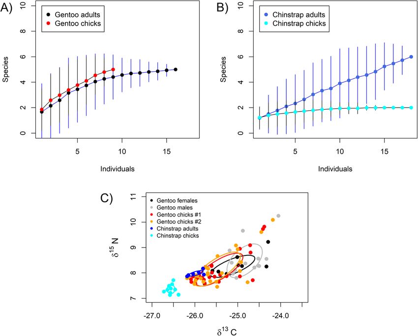
ves, Table 2). 0.028; R2 = 0.10; Additional file 1, Fig. S24). Gentoo
chicks had a slightly richer diet composition than adults,
Calculation of energy as they were fed more frequently with fish (Fig. 5a,
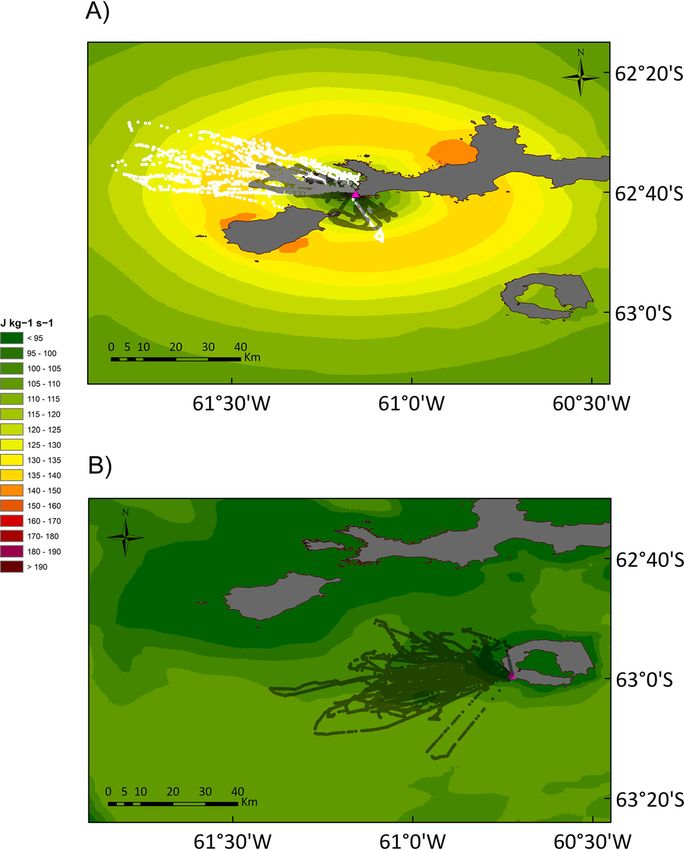
Gentoos from Livingston used areas of the energy land- Table 3). In chinstraps, chicks were fed more frequently
scape that resulted in the lowest foraging costs relative with Thysanoessa macrura, which is taken only very oc-
to energy gain during foraging (up to 137.6 J kg− 1 s− 1), casionally in adults, and adults had a richer diet compos-
avoiding areas equally distant where the costs were ition by consuming occasionally some fish (Fig. 5b,
higher (150 to 160 J kg− 1 s− 1, Fig. 3a). Moreover, the en- Table 3). However, permutation tests were not signifi-
ergy landscapes in the marine areas around Livingston cant when gentoos (F24,1 = 1.4, P = 0.203, R2 = 0.059) or
(Fig. 3a) implied much lower costs than those around chinstraps (F35,1 = 1.1, P = 0.254, R2 = 0.032) were ana-
New Island (up to 232 J kg− 1 s− 1, Additional file 1, Figs. lysed apart (Additional file 1, Figs. S25, S26).
S20 to S22). During short trips, gentoos from Livingston
incurred in foraging costs per bottom time gain with a Stable isotope analysis of the diet
median value of 115.2 J kg− 1 s− 1 (94.9 to 136.7, Fig. 4a). Mean isotope values differed among the Antarctic
The median foraging cost per bottom time gain during penguin groups (Kruskal Wallis ANOVA for δ13C:
the long trips performed by gentoos from Livingston χ2 = 35.1, d.f. = 5, P < 0.001, for δ15N: χ2 = 46.9, d.f. =
was 130.5 J kg− 1 s− 1 (95.3 to 137.6, Fig. 4b). In the case 5, P < 0.001; Fig. 5c, Additional file 1, Table S11). In
of New Island, gentoos incurred in variable foraging gentoos, the differences in δ13C signature were related
costs per bottom time gain: 1) South End colony 2013, to higher values in adult males than in chicks (Fig.
167.1 (106.1 to 232.0; Fig. 4d), 2) South End 2014, 112.7 5c, Additional file 1, Table S11), indicating a more
(78.7 to 183.1, Fig. 4e), 3) North End 2014, 99.0 (82.9 to benthic diet for adults, as also shown by the analyses
151.9, Fig. 4f) (medians and ranges in J kg− 1 s− 1). In this of dive parameters in Table 2. Gentoos had also sig-
way, the foraging costs per bottom time gain of the short nificantly higher δ13C than chinstraps (Fig. 5c, Add-
trips were lower than those of the long trips, while those itional file 1, Table S11), indicating again a more
from New Island South 2013 were the highest and those benthic diet for gentoos, in line with the significant
from New Island North End 2014 the lowest (Kruskal- differences in dive parameters (Table 2). In the case
Wallis χ2 = 23,852, d.f. = 5, P < 0.001; pairwise analyses of δ15N, the differences among the groups were re-
in Additional file 1, Table S9). lated to higher values in chinstrap adults than in their
Chinstraps used marine areas around Deception where chicks (Fig. 5c, Additional file 1, Table S11), which is
the foraging costs per bottom time gain were below 105 J in line with the observation that chinstrap chicks
kg− 1 s− 1 (median 96.5, range 80.8 to 103.7; Figs. 3b and were only fed with Euphausiacea (Table 3; Additional
4c). Chinstraps incurred significantly lower foraging costs file 1, Fig. S26). All niche metrics (Fig. 5c, Additional
per bottom time gain than the gentoos from Livingston file 1, Table S11) were larger in gentoos than inYou can also read