GABI DATABASES 2019 EDITION - UPGRADES & IMPROVEMENTS - GABI SOFTWARE
←
→
Page content transcription
If your browser does not render page correctly, please read the page content below
Please read this document carefully, as it contains:
 - Important information regarding changes in the databases
 - Details on changes in process datasets and on cross-cutting changes
 - Information on new datasets
 - Information on discontinued datasets

GaBi Databases
2019 Edition
Upgrades & improvements

                                                    February 2019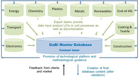
About this document

This document covers relevant changes in the upgraded LCI datasets of the GaBi Databases. The
document will address both methodology changes and changes in technology, if any, and is struc-
tured by material or topic, e.g., electricity, metals, plastics, renewables. It also covers newly added
datasets to the database.

In the Annex you will find the list of datasets that are no longer updated.

thinkstep uses a professional issue tracking software (JIRA), so the issue numbers in the tables are
issue numbers from this software.

Key changes and affected datasets

In the following paragraphs, you will find a short summary of the most important changes that
took place in this year’s upgrade.

Important database-wide changes made in the 2019 database edition include:

-   Energy update: all energy-related datasets, such as electricity, thermal energy, fuels and
    the like, have been updated in line with the latest available, consistent international energy
    trade and technology data. Please see Chapters 2.6 and 2.7 for more information.
-   Land use: Land use for underground mining has been implemented in the database.
-   Capital goods: Building infrastructure is now implemented for waste water treatment, com-
    plementing the situation for the various types of renewable and fossil power plants and for
    waste incineration. Separate datasets for transport infrastructure and production sites are
    available, which now allow users to calculate the impact of building infrastructure consist-
    ently throughout the entire life cycle.
-   Halogenated substances: Since the use of certain halogenated substances has been
    banned following the implementation of the Montreal Protocol, the following emissions are
    not present anymore in the updated thinkstep datasets: Halon (1301), R 11 (trichlorofluo-
    romethane), R 114 (dichlorotetrafluoroethane) and R 12 (dichlorodifluoromethane) and R
    22 (chlorodifluoromethane). Particularly R22, which has been removed, has the profound
    effect of reducing the remaining, already greatly reduced ODP impacts by several orders
    of magnitude for most datasets. This consequently further reduces the impact results for
    ODP for many datasets in the database.
-   Primary energy correction of wood and wood-based datasets: when using an economic al-
    location along the life cycle, primary energy needs to be adjusted to guarantee a proper energy
    balance. For wood and wood-based datasets, the primary energy has been adjusted accordingly,
    based on the fresh mass of the related material considering the upper calorific value (measured
    at oven-dry status and upscaled linearly for water content). The related elementary flow docu-
    menting the renewable primary energy is the flow “Primary energy from solar energy.”
                                                   2
Additionally, the following issues resulted in noteworthy changes, which we would like to high-
light:
- Update of the quantity “Price”: The quantity “Price” was updated using mainly Euro-
stat data, and some unit conversion errors have been corrected. This leads to certain
changes in the database, where economic allocation on these specific flows is used.
However, concerning the update of GaBi datasets, the change due to this price update
was mostly moderate to low. For a complete list of the changes, please see the table
in Annex III of this document. 1
- BF Steel water balance: The topic of water assessment in LCA generally made a
significant step toward better definition and standardization of methods and character-
ization. Therefore, the water balance of BF steel could be improved. To close the water
balance of the blast furnace steel route, rain water was added and the blue water con-
sumption double checked and corrected in relationship to the most recent water ele-
mentary flows. Previously too, a lot of water was being emitted compared to the water
entering production. This has now been corrected. This change led to an improvement
toward a correct water balance and blue water consumption (for some steel sheet and
steep pipe datasets, the blue water consumption changed from negative to positive
values, from about -0.7 kg to 1.4 kg per kg of product).
- Infrastructure and land use information for waste incineration: For waste incinera-
tion, building (as capital good) and land use information was added. This addition
slightly increases the impact of all waste incinerations and introduces land use values
for this step. In waste incineration for ferro metals, another effect appears that de-
creases the (overall very small) impact of GWP by another 30%. Ferro metals do not
cause CO2 emissions because of the lack of substantial embodied C and only during
the consumption of auxiliary energy to run the plant. Therefore, the crediting of the
recovered iron components is influencing the overall low absolute GWP value. The
1
Any update will overwrite prices that have been changed by clients. Should this affect you and to avoid this in the future, please always
create own quantities for your needs.
3effect is caused by slight change in the supply chain logistics of the recovered—and
thus credited—iron ore and certain regionalization effects of the applied waste water
treatment.
- Waste water treatment plant update: Due to our cooperation with End-of-Life experts
from TH Bingen, this year the waste water treatment plants received an update and
correction. With new advancements in measuring technology leading to new data from
a relevant scientific paper, diffuse emissions to air could now be included. Infrastructure
and land use were added to the datasets for consistency purposes, however they do
not significantly influence the overall results. Electricity consumption and the most im-
portant emissions to water could now be matched with the latest DWA (Deutsche Ver-
einigung für Wasserwirtschaft, Abwasser und Abfall e.V.) statistics for German waste
water treatment plants in 2016. Additionally, the calculation of the sludge output of the
pre-thickening and dewatering was recalculated and consistently reduced, as prior as-
sumptions could be identified as being too conservative. In the supply chain, a waste
water plant is generally of rather low absolute significance. Therefore, even slight
changes in details cause high relative changes in the waste water plant as such. The
sludge update leads to a relative decrease of about 80% of the GWP. When applicable,
regional waste water treatment plants are now used in the country-specific datasets.
This change especially improves the precision of US-specific datasets in the EP cate-
gory, where impacts increase due to the regional differentiation.
- Use of global copper dataset: Copper is produced and traded globally. In order to be
more representative, the GLO: copper mix dataset will replace the German copper mix
dataset. This substitution mainly influences the AP and PM impact categories, and de-
pending on the amount of copper used, the impacts will increase moderately to sub-
stantially (up to a maximum of 150% for AP and 140% for PM).
- German cement update: The German cement datasets have been updated using in-
formation from VDZ (Year 2015). 2 The main changes were done in the clinker produc-
tion, such as with the fuel mixture and emissions update. The resulting decrease can
be seen mainly when looking at Portland Cement: here AP decreases by about 40%,
POCP by about 30% and EP by about 15%.
- Update of ships: Emission factors were updated and now use consistently data ac-
cording to the IMO GHG report 2014. 3 The fuel consumption calculation related to DWT
was updated and new discrete fuel consumption values from IMO GHG report 2014
2
VDZ Umweltdaten 2015
3
Third IMO Greenhouse Gas Study 2014
4are now used. Impacts decrease slightly overall, except for the category related to par-
ticle emissions, where the impacts increase up to 90% because of the updated emis-
sion factors.
- US trucks update: Relevant emission factors from EPA MOVES have been used to
update the US truck datasets. Apart from updating existing emission factors in these
US datasets, additional ones, such as Benzene and Nitrogen monoxide for VIUS da-
tasets and benzene and ammonia for SmartWay datasets, have been added. CO2 and
SO2 calculations remain unchanged, because they are calculated from fuel consump-
tion and are not based on emission factors from MOVES.
- End-of-Life update of building technology: End-of-Life for building technology da-
tasets were updated, as the amount and kind of used steel in the initial production was
harmonized with the related amount of steel and stainless steel in EOL for more appro-
priate crediting concerning the different recovered steel types.
- Aluminium: For datasets from Brazil and Ukraine, the ingot production was updated.
Recently available and updated IAI data was used.
- Gypsum mining: Dust emissions were added to the mining step. Now the gypsum
mining - like all other mineral mining processes in GaBi - is also inventoried with the
related dust emissions consistently.
- Update of Australian EPDs: 45 new EPD datasets from FWPA in Australia are now
available in addition to over 100 updated ones in the Professional database.
Further details and the related rationale are provided in Chapters 2 ff.
5Authors:
Dipl.-Ing. Steffen Schöll steffen.schoell@thinkstep.com
Dipl.-Geoökol. Ulrike Bos ulrike.bos@thinkstep.com
MSc. Morten Kokborg morten.kokborg@thinkstep.com
Prof. Dr.-Ing. Thilo Kupfer thilo.kupfer.ext@thinkstep.com
Dr.-Ing. Martin Baitz martin.baitz@thinkstep.com
Dr. Lionel Thellier lionel.thellier@thinkstep.com
Dipl.-Ing. Alexander Stoffregen alexander.stoffregen@thinkstep.com
Dipl.-Ing. Jasmin Hengstler jasmin.hengstler@thinkstep.com
Dr.-Ing. Marc-Andree Wolf marc-andree.wolf.ext@thinkstep.com
______________________________________________________________________________________________________________________________________________
thinkstep AG
Hauptstr. 111 – 113, 70771 Leinfelden-Echterdingen, Germany
Phone: +49 711 341 817-0 Fax: +49 711 341 817-25
E-mail: info@thinkstep.com
Websites: www.thinkstep.com www.gabi-software.com
_______________________________________________________________________________________________________________________________________________
6List of Contents
List of Figures ....................................................................................................... 9
List of Tables ........................................................................................................ 9
Abbreviations ...................................................................................................... 10
1 Introduction to the upgrade of databases available with GaBi .......... 11
2 GaBi Databases 2019 Edition ............................................................... 12
2.1 Principles ........................................................................................................... 12
2.2 Reasoning behind this document ....................................................................... 13
2.3 Regionalization .................................................................................................. 14
2.3.1 Land Use ........................................................................................................... 14
2.3.2 Regionalized Water ........................................................................................... 14
2.4 LCIA Method and factor updates and corrections .............................................. 14
2.4.1 ISO 14067 for GHG reporting ............................................................................ 14
2.4.2 Environmental Footprint (EF) ............................................................................. 14
2.4.3 Single substances.............................................................................................. 15
2.5 New datasets ..................................................................................................... 17
2.6 Inventories for electricity, thermal energy and steam ......................................... 18
2.7 Inventories for primary energy carriers............................................................... 32
2.8 Organic and inorganic intermediates.................................................................. 36
2.9 Inventories for metal processes ......................................................................... 41
2.10 Inventories plastic processes ............................................................................. 43
2.11 Inventories for End-of-life processes .................................................................. 44
2.12 Inventories for electronic processes ................................................................... 46
2.13 Inventories for renewable processes.................................................................. 48
2.14 Inventories for transport processes .................................................................... 51
2.15 Inventories for construction processes ............................................................... 54
2.16 Inventories for US regional processes ............................................................... 58
3 Industry data in GaBi ............................................................................. 62
4 General continuous improvements ...................................................... 67
4.1 Editorial ............................................................................................................. 67
4.2 LCIA Methods, Normalisation and Weighting factors ......................................... 68
4.3 Fixing and improvements of cross cutting aspects ............................................. 71
References .......................................................................................................... 75
7Annex I: “Version 2018” discontinued datasets – Explanations and
Recommendations ................................................................................. 76
Annex II: EPDs with expired validity ................................................................. 82
Annex III: Price quantity changes ..................................................................... 84
Annex IV: Biogenic carbon content quantity changes .................................... 88
8List of Figures
Figure 1: Process structure in GaBi databases 11
Figure 2: Development grid mix in Germany (left) and EU-27 (right) [Eurostat 2018] 19
Figure 3: Development grid mix United States [EIA 2017] 19
Figure 4: PED, GWP, EP, POCP and AP of electricity grid mixes DE, EU-27 and US 24
Figure 5: Changes in GWP of electricity grid mix datasets in GaBi Professional 2019
Edition 25
Figure 6: Absolute GWP of electricity grid mix datasets in GaBi Professional 2018 &
2019 Edition 25
Figure 7: Development GWP for electricity supply in selected countries 28
Figure 8: Changes in GWP electricity grid mix datasets in GaBi Extension Module
Energy 2019 28
Figure 9: Absolute GWP of electricity grid mix datasets in GaBi Extension module
Energy 2018 & 2019 29
Figure 10: Development GWP for electricity supply in selected countries 29
Figure 11: Absolute GWP of electricity grid mix datasets in GaBi Extension module
Full US 2018 & 2019 30
Figure 12: Changes in GWP electricity grid mix datasets in GaBi Extension Module
Full US 2019 31
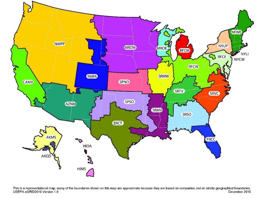
Figure 13: 26 eGRID subregions 32
List of Tables
Table 1: Energy carrier mix for electricity generation—selected EU countries
(calculated based on [IEA 2018]) 20
Table 2: Energy carrier mix for electricity generation—selected non-EU countries
(calculated based on [IEA 2018]) 20
Table 3: Energy carrier mix for electricity generation—countries with significant
changes (calculated based on [IEA 2018]) 21
9Abbreviations
AP Acidification Potential
ADP Abiotic Depletion Potential
BAT Best Available Technique
B2B Business-to-Business
B2C Business-to-Customer
CHP Combined Heat and Power Plant
CML Centrum voor Milieuwetenschappen (Institute of Environmental Sciences)
EF Environmental Footprint
EP Eutrophication Potential
EPS Environmental Priority Strategies (LCIA method)
EPD Environmental Product Declaration
GWP Global Warming Potential
ILCD International Reference Life Cycle Data System
LCA Life Cycle Assessment
LCI Life Cycle Inventory
LCIA Life Cycle Impact Assessment
ODP Ozone Depletion Potential
PED Primary Energy Demand
POCP Photochemical Ozone Creation Potential
UBP Umweltbelastungspunkte (Ecological Scarcity Method)
For chemical elements, the IUPAC nomenclature is applied. Country codes use the ISO 3166-1
alpha 2 2-letter code, plus a few 3-letter codes for regions, such as RER for Europe, RNA for North
America and GLO for global. The different combinations of the European Union, reflecting its growth
over time, are identified by the prefix EU and the Number of Member States (potentially plus “EFTA”
when including the countries of the European Free Trade Association, i.e., Iceland, Liechtenstein,
Norway and Switzerland).
101 Introduction to the upgrade of databases available
with GaBi
In total, around 50 thinkstep employees were involved in the upgrade of several thousand unit pro-
cesses and aggregated LCI datasets. The invested time, knowledge and dedication of our employees
resulted in the new GaBi Databases 2019 Edition, with about 12,500 plans and processes of the
regular Professional and Extension Databases, plus more than 2,000 processes as Data-on-Demand-
only datasets.
The process of continuous upgrades to the GaBi Databases is enabled and supported with domain
expertise along the team structure within thinkstep, which is illustrated in the figure below.
Figure 1: Process structure in GaBi databases
In the GaBi Databases, process documentation is directly integrated in the datasets. Additional infor-
mation about the modelling principles applied to all datasets can be found in the document GaBi Da-
tabases and Modelling Principles. 4 Furthermore, specific modelling information on specific topics can
equally be accessed on the GaBi Software website.
This document covers relevant changes in the upgraded LCI datasets of the GaBi Databases. The
document will address both methodology changes and changes in technology, if any, and is structured
by material or topic, e.g., electricity, metals, plastics, renewables. In general, all thinkstep-related da-
tasets have been upgraded.
4
http://www.gabi-software.com/index.php?id=8375
11Methodological changes do not automatically imply endorsement by thinkstep, but have been intro-
duced when necessary. Methodological changes are only useful if these changes or improvements
are supported by relevant best practise cases, evolving or edited standards or by relevant stakeholder
initiatives with a respective practice approval.
2 GaBi Databases 2019 Edition
“Facts do not cease to exist because they are ignored.” – Aldous Huxley
2.1 Principles
thinkstep introduced the annual upgrade of the GaBi databases for three reasons:
• To keep your results as up-to-date and close to evolving supply chains as possible, including
automated upgrades of your valued work in alignment with the most current state.
• To avoid disruptive changes caused by multi-year intervals that are often hard to communicate
and interpret and that prolong the time that user results are affected by known data errors.
• To keep track of necessary methodological changes and implement them promptly.
thinkstep’s databases are based on technical facts and are internationally accepted and broadly ap-
plied. We preferably use standardized methods established by industry, science and regulatory au-
thorities. New methods are applied when they have proven to be based on a relevant standard, on
broadly and internationally accepted approaches or when enforced by relevant regulations.
Changes in datasets are often the result of many effects in supply chains. But “technical” reasons
should be carefully separated from methodological reasons. Necessary methodological adoptions due
to evolving standards, knowledge and frameworks may be useful, however, GaBi databases do not
undertake methodological trials on the basis of databases that aim to reflect technological reality.
Changes in the environmental profile of the datasets, from the predecessor GaBi Databases to the
most recent GaBi Databases, may be attributed to one or more of the following factors:
• Upgrade of the foreground and/or background systems. The market situation or newly
available technologies result in changed impacts. The environmental profile for the supply of
energy carriers or intermediates may be subject to short-term changes and affect the environ-
mental profile of virtually all materials and products to a varying extent. For example, a change
of the energy carrier mix or of the efficiency for electricity supply, changes the environmental
profile of all materials or products using that electricity supply.
• Improvements and changes in the technology of the production process. Improvements
or developments in production processes might achieve, for example, higher energy efficiency
or a reduction of material losses and of process emissions. Sometimes, the technology is sub-
jected to higher quality requirements that are defined further downstream at the final product-
level (e.g., more end-of-pipe measures to reduce emissions, stricter desulphurization of fuels)
and improved use phase performance. In addition, certain production routes might have been
phased out, have changed the production mix of a material, substance or energy. A frequently
12changing and quite dynamic example are the electricity grid mix datasets, as some countries
reduce or phase-out certain types of energy or fuels in the electricity supply mix, which require
the introduction of alternative sources of fuels and energy.
• Further standardization and the establishment of regulative modelling approaches.
Modelling of realistic technology chains has always been the core focus of the GaBi database.
Further harmonization and improvement in the LCA methodology and feedback from clients
and employees have enhanced the modelling approach for the GaBi Databases. Detailed in-
formation is given in the document GaBi Databases and Modelling Principles. 5 Methodological
adoptions are carried out extremely carefully, passing through multiple levels of reviews by
thinkstep experts responsible for standardization, technology knowledge and quality assur-
ance. This internal review process was audited within the continuous improvement process by
our external verification partner DEKRA. GaBi database updates and upgrades focus on reli-
ability through consistency to ensure clients system models and results are not jeopardized
due to random methodological changes.
The degree of influence of each of these factors is specific to each process and cannot be generalized
for all cases, nor can a single factor be highlighted. However, as technological excellence is a core
value of thinkstep data, our focus is to update and apply ALL RELEVANT AND IMPORTANT improve-
ments and changes in technology and the supply chain and THE NECESSARRY AND ESTABLISHED
improvements and changes in the methodology.
Supply chain modelling of a single material involves hundreds or even thousands of single operations.
Therefore, even opposing effects (improvements of some processes and higher impacts of other pro-
cesses along the chain) may occur.
2.2 Reasoning behind this document
GaBi systems—e.g., leading to a single aggregated dataset—consists of multiple datasets within one
supply chain. This means, users could identify many reasons for changes within a single supply chain.
GaBi models must be able to reflect, in first instance, the necessary complexity of the reality to provide
realistic data. Reduction of complexity is only credible if the reality of the supply chains is still ade-
quately mirrored. The change analysis is a time consuming, but important process within thinkstep,
and the results are documented in this report.
However, the relevance of changes in the GaBi database related to the user’s own systems is highly
dependent on the goal and scope in the specific user application. This means the same dataset may
lead to significant changes for one user, whereas in another user’s system, the changes might be
irrelevant. To shorten the time for users to reflect on the relevancy of the GaBi database changes for
their own systems, the analyst function of GaBi Software may support you in an effective way. As a
means of guiding users to the relevant changes in their models that are due to changes in external
factors and GaBi background data upgrades, thinkstep also provides the present document “GaBi
Databases 2019 Edition - Upgrades and Improvements” in addition to the document “GaBi Databases
5
http://www.gabi-software.com/index.php?id=8375
13and Modelling Principles,” complemented by close to 14,000 interlinked electronical documentation
files of the processes supplied with thinkstep databases.
The following sections will address the most relevant changes in the GaBi Databases for the different
areas.
2.3 Regionalization
2.3.1 Land Use
For land use assessment, the regionalization in mining and renewable resources datasets (agricultural
and wood biomass) as well as incineration, which cover the most important sectors of land occupation
and transformation, was further implemented and harmonized. Land use inventory flows for all culti-
vation and forestry processes as well as mining and waste incineration processes were checked and
updated, and missing information has been integrated. Land occupation [m²*a] and land transfor-
mation [m²] inventory information for mining processes were improved through updating the produc-
tion quantity and size of open pit mines and implementing land use flows for underground mining.
Furthermore, the occupied land use mining area was separated into “dump site”, “mineral extraction
site” and industrial area.” Thus, a more complete and further differentiated evaluation of land use
impacts is possible.
2.3.2 Regionalized Water
The regionalization of water flows was further implemented and expanded to the waste water treament
plants. The input and output water flows (input: ground water, river water, lake water; output: pro-
cessed water to groundwater, processed water to lake, processed water to river) are regionalized by
the country of the waste water treatment plant.
For further information regarding water assessment and how to ensure correct and coherent region-
alization at the input and output side, please see documentation in “Introduction to Water Assessment
in GaBi.”
2.4 LCIA Method and factor updates and corrections
2.4.1 ISO 14067 for GHG reporting
Four new quantities from ISO 14067 GWP (based on IPCC AR5) are now available. They use the
same characterization values as IPCC AR5, but split into fossil, biogenic, land use and aviation.
2.4.2 Environmental Footprint (EF)
The Environmental Footprint (EF) set of impact factors have been updated to version 2.0. Apart from
various more specific changes, the most visible update is the introduction of three sub-impacts to
climate change, namely fossil, biogenic and land use. These three impacts sum up to the total impact.
IMPORTANT NOTE:
14With release of the GaBi Databases 2019 Edition, the official EF 2.0 characterisation factors are pro-
vided, as well as the mapping to the official units and official elementary flows via the ILCD export/im-
port function.
EF 2.0 is the only version to be used for PEF/OEF results and to create EF data as ILCD export file.
Do not use previous versions of EF characterisation factors and ILCD zip archives anymore! Earlier
versions of EF/ILCD LCIA methods and flow lists have no official status and datasets developed with
earlier versions may not be claimed EF-compliant. In case you have been using a previous version
of EF characterisation factors, please update any created dataset by re-export, respectively re-
calculate results using the EF 2.0 in GaBi (datasets created by users should also be double-
checked with recent official EF documents, before claiming compliance). In case you need any
support with this topic, please contact content@thinkstep.com
Additional information: EF 3.0 is in parallel online at the EC website, since December 2018. This
version may be used exclusively in context of new to-be-developed PEFCRs/OEFSRs in the transition
phase (and is hence not yet included in GaBi).
2.4.3 Single substances
• GWP characterization factors for the substances HCFC 142b and R 134a were corrected.
• Long-term emission of halogenated substances flows carry now GWP factors: R 134a (tetra-
fluoro ethane), R 143a (trifluoroethane), R 113 (trichloro trifluoroethane), R 141b (dichloro-1-
fluoroethane), R 152a (difluoroethane), R 114 (dichlorotetrafluoroethane), R 142b (chlorodi-
fluoroethane), R 124 (chlorotetrafluoroethane), R 115 (chloropentafluoroethane), R 116 (hex-
afluoroethane), R 125 (pentafluoroethane), Halon (1211), Halon (1301), R 13 (chlorotrifluoro-
methane), R 32 (difluoromethane), Tetrafluoromethane.
• A set of characterization factors for unspecified Cresol were calculated as an average of the
three isomers (ortho-, meta- and para-cresol) for ReCiPe, CML and USEtox.
• The long-term emissions of phosphorus are now available for several impact categories.
• The energy flow ‘Gas, mine, off-gas, process, coal mining’ used to be characterized via the
net calorific value in primary energy categories similar to, for example, natural gas in the GaBi
implementation of EF 1.8. However, the flow is not present in the official list of characterization
factors from EF 1.8 and EF 2.0 and has now been removed.
• Ecoinvent provided updated calorific values for three elementary energy flows which increased
by 30-50% in the Ecoinvent 3.5 database: hard coal, brown coal and peat. The primary energy
characterization of these flows will increase. Crude oil and natural gas changed very little (2-
3%).
• Several land use flows related to GWP were re-introduced into the GaBi database to remain
consistent with the EF2.0 flow list:
o Carbon dioxide, from soil or biomass stock (long-term)
o Carbon monoxide, from soil or biomass stock
o Carbon monoxide, from soil or biomass stock (long-term)
o Methane, from soil or biomass stock
o Methane, from soil or biomass stock (long-term)
15• UK land use flows are removed, because they were already present as GB flows. The differ-
ence in land use characteristics between the two (Great Britain vs United Kingdom) is assumed
negligible.
• Land use flows without regional specification in the LANCA methodology were regionalized,
some causing changes of 30-100% to the LANCA impacts.
• The EPD flows PERM, PENRM, PERE and PENRE have been deleted. They are not used in
EPD-pilot solutions and carry a significant risk of double counting primary energy if not used
properly.
• Water flows with regional characterization were added for Saudi Arabia
• EPD EN 15804 flows were not linked to the respective EN 15804 impacts—this has been
corrected. If GaBi users were implementing EPD results directly using the EN 15804 flows,
these were previously ignored, but are now characterized. This is only relevant if users were
manually implementing finished EPD results (LCIA results). No standard datasets were af-
fected.
• Waste heat [Other emissions to air] had a characterization factor for POCP in ReCiPe 2016
v1.1, which was removed.
• SOx was not characterized as emission in ReCiPe 2016 v1.1 and is now corrected.
• Four water input flows used in the Ecoinvent database were a factor of 1,000 too low in the
WSI and AWARE water methodologies. Since output flows were correctly characterized, this
led to negative water consumption for Ecoinvent processes. This has been corrected.
• The Ecoinvent flow for water and turbine use, unspecified natural origin was wrongly charac-
terized in the GaBi implementation of UBP 2013 water resource quantity, leading to negative
water consumption for Ecoinvent processes. This has been corrected.
• Other water flows were corrected in UBP2013 leading to a 30-50% decrease in the character-
ized water footprint.
• Land use flows to/from/use as permanent crops in Costa Rica were not characterized in
LANCA, which has now been corrected.
• Phosphorus as emissions to water (P total) had mistakingly received a toxic classification in
ReCiPe 1.08. This has been corrected, leading to a nearly 100% decrease in toxicity for this
specific flow. Other impact methods are not affected.
• CAS number of 1-butene was corrected to 000106-98-9 with 025167-67-3 as synonym.
• Butane and iso-Butane both with CAS 000075-28-5 were merged and characterization factors
aligned.
• CAS code of SO3 was corrected from 007746-11-9 to 007446-11-9.
• Two flows of tin ore were not consistently characterized. The flows were merged.
• Vulcanized natural rubber had wastewater emissions set as water vapour. This has been cor-
rected.
• Flow duplicates were merged:
o Aldehydes to fresh water
o Aluminium to air
o Aluminium to sea water
16o Sodium to fresh water
o Sodium to industrial soil
o Sodium to agricultural soil
• Phosphorus minerals had been characterized for resource depletion with the inverse value
(1.81E05 instead of 5.52E-06) in ‘CML’ and ‘ILCD 1.09 Resource use, minerals and metals’
and was corrected. The effect could go from being completely dominating on the resource
depletion to being close to zero.
• The name of the flow Butylglycol was changed to 2-Butoxyethanol
2.5 New datasets
With this year’s upgrade, 379 new processes and 141 new plans are available:
Professional DB:
3 new plans, 162 new processes
Third party datasets, GLO: copper mix, production of ships, different electricity,
regionalized tap water…
Extension DBs:
II “Energy”: 1 new plan, 84 new processes
Future electricity grid mixes (2025, 2030, 2040), gasoline mix E5 and E10, differ-
ent “EU-28 electricity from …” mixes
IXa “End of Life”: 13 new processes
Bulk waste truck, US: hazardous waste incineration plants, open biomass burn-
ing,…
New extension database IXb “End of Life parametrized models”:
137 new plans, over 40 unique new processes, plus many complementing pro-
cesses of energy sources, consumables, for crediting
XIV “Construction”: 24 new processes
CN/BR/SA Portland cement, several EPDs
XVII “Full US”: 27 new processes
Different waste incineration plants, Iron ore mix…
XX “Food&Feed,” XXI ”India,” XI “Electronics,” Ib “Inorganics”: jointly 25
new processes
IC produced in India, corn and grain drying, Ammonia, canola oil…
17Details on the new datasets are available in this MS Excel file: http://www.gabi-software.com/filead-
min/GaBi_Databases/Database_Update_2019_DB_content_overview.xlsx and access to the com-
plete dataset documentation is available for searching and browsing by extension database online
under http://www.gabi-software.com/international/databases/gabi-data-search/.
2.6 Inventories for electricity, thermal energy and steam
Relevant changes in energy carrier mix for electricity generation after the upgrade
In the GaBi databases 2019, the reference year is 2015 for all electricity grid mixes and energy
carrier mixes. As an exception, the electricity grid mixes in the Extension Module XVII: Full US
(electricity grid mixes for US sub-grids and subregions under eGRID) have been updated from
reference year 2014 to 2016, using the most recent version of eGRID [EPA 2018].
Relevant changes in the life cycle inventory (LCI) of the upgraded national grid mix datasets
occur for a couple of countries, because of changes in the energy carriers that were used for
electricity generation, as well as changes in the amount of imported electricity and the country
of origin of these imports. The changes in the LCI data sets reveal the following trends:
• An ongoing trend in some countries is to increase the share of renewable energy in their
electricity generation, which is the case for Austria, Belgium, Denmark, Estonia, Finland,
Germany, Great Britain, Greece, Ireland, Lithuania, Romania and Sweden, for example.
• Annual fluctuation in electricity generation from hydropower (availability of water for elec-
tricity generation) due to meteorological conditions. In 2015, lower water availability for
hydropower compared to 2014 resulted in higher shares of fossil fuels, for example in
Austria, Croatia, Italy, Latvia, Portugal, Serbia, Slovenia and Venezuela. In contrast,
higher water availability in Finland, Sweden and Turkey resulted in distinct higher elec-
tricity output from hydro power plants.
• As in previous years, several transition countries have an ongoing demand for increased
electricity production: In countries like China, India, Egypt, Saudi-Arabia, Vietnam or Tur-
key, electricity production has increased by 4 to 12%. In China, in contrast to previous
years, the extra electricity demand was not covered by electricity from coal. Around one
third of the 180 TWh of the increased electricity generation (5,860 TWh total gross pro-
duction) was generated by hydropower. The remaining increase in China was predomi-
nantly generated from nuclear, wind, natural gas and photovoltaic. In India, Egypt, Saudi
Arabia and Vietnam, the increased electricity demand was met by production from fossil
fuels, mostly coal or natural gas.
The following three figures present the development of the energy carrier mix for electricity gen-
eration in Germany, the European Union and the United States between 2000 and 2015.
18Figure 2: Development grid mix in Germany (left) and EU-27 (right) [Eurostat 2018]
Figure 3: Development grid mix United States [EIA 2017]
Compared to 2014, the use of renewable energy sources for electricity generation in Germany
has increased from 27.0% to 30.0% 6 in 2015. The main driver of this increase in renewable
energies was electricity from wind. Generation from combustible, fossil fuels decreased from
56.4% to 54.7%.
For the EU28, the share of natural gas in the power mix increased from 14.5% in 2014 to 15.5%
in 2015, after a significant reduction from 22.8% in 2010. The generation from renewable energy
6
50 % of electricity from waste is accounted as renewable energy
19carriers increased slightly, from 29.4% in 2014 to 30.0% in 2015. The increase was mainly driven
by an increase in wind power generation.
In the U.S., the trend of coal substitution by natural gas was also happening in 2015, decreasing
the share of coal use in the grid mix significantly, from 38.5% to 33%. The share of natural gas
for electricity generation increased from 27.4% to 32.5%.
In the following tables, the energy carrier mixes for 2014 and 2015 are displayed for selected,
economically most-relevant countries, or those with important changes.
Table 1: Energy carrier mix for electricity generation—selected EU countries (calculated based on [IEA
2018])
France Germany Great Britain Italy Poland Spain
[ %]
2014 2015 2014 2015 2014 2015 2014 2015 2014 2015 2014 2015
Nuclear 77.6 77.0 15.5 14.2 18.8 20.7 0.0 0.0 0.0 0.0 20.6 20.4
Lignite 0.0 0.0 24.9 23.9 0.0 0.0 0.3 0.3 33.6 32.0 1.1 1.2
Hard coal 1.7 1.7 19.0 18.3 29.8 22.3 15.2 15.0 47.9 47.1 14.7 17.1
Coal gases 0.4 0.4 1.7 1.8 0.3 0.3 1.1 0.8 1.3 1.5 0.5 0.5
Natural gas 2.3 3.5 10.0 9.8 29.7 29.5 33.5 39.3 3.4 3.9 17.0 18.7
Heavy fuel oil 0.3 0.4 0.9 1.0 0.5 0.6 5.1 4.7 1.0 1.3 5.1 6.1
Biomass (solid) 0.3 0.4 1.9 1.7 4.1 5.7 1.4 1.4 5.8 5.5 1.4 1.4
Biomass (Biogas) 0.3 0.3 5.0 5.2 2.4 2.1 4.5 4.6 0.5 0.6 0.3 0.3
Waste 0.7 0.7 2.2 2.0 1.2 1.9 1.7 1.7 0.0 0.0 0.5 0.5
Hydro 12.3 10.5 4.1 3.9 2.6 2.7 21.6 16.6 1.7 1.5 15.4 11.2
Wind 3.1 3.7 9.2 12.3 9.4 11.9 5.4 5.3 4.8 6.6 18.7 17.6
Photovoltaic 1.1 1.3 5.8 6.0 1.2 2.2 8.0 8.1 0.0 0.0 2.9 2.9
Solar thermal 0.0 0.0 0.0 0.0 0.0 0.0 0.0 0.0 0.0 0.0 2.0 2.0
Geothermal 0.0 0.0 0.0 0.0 0.0 0.0 2.1 2.2 0.0 0.0 0.0 0.0
Peat 0.0 0.0 0.0 0.0 0.0 0.0 0.0 0.0 0.0 0.0 0.0 0.0
Table 2: Energy carrier mix for electricity generation—selected non-EU countries (calculated based on
[IEA 2018])
20Brazil China India Japan Russia USA
[ %]
2014 2015 2014 2015 2014 2015 2014 2015 2014 2015 2014 2015
Nuclear 2.6 2.5 2.3 2.9 2.8 2.7 0.0 0.9 17.0 18.3 19.2 19.3
Lignite 1.3 1.3 0.0 0.0 15.6 11.3 0.0 0.0 5.7 5.7 2.1 2.0
Hard coal 1.8 2.0 71.1 68.8 59.3 63.9 29.8 29.3 8.6 8.6 37.3 32.1
Coal gases 1.4 1.4 1.3 1.3 0.1 0.1 3.7 3.7 0.4 0.5 0.1 0.1
Natural gas 13.7 13.7 2.0 2.5 4.9 4.9 40.4 39.4 50.1 49.6 26.8 31.8
Heavy fuel oil 6.0 5.0 0.2 0.2 1.8 1.7 11.2 9.8 1.0 0.9 0.9 0.9
Biomass (solid) 7.7 8.3 0.8 0.9 1.8 1.7 2.8 3.3 0.0 0.0 1.1 1.1
Biomass (Biogas) 0.1 0.1 0.0 0.0 0.1 0.1 0.0 0.0 0.0 0.0 0.3 0.3
Waste 0.0 0.0 0.2 0.2 0.1 0.1 0.6 0.7 0.3 0.3 0.4 0.4
Hydro 63.3 61.9 18.7 19.3 10.2 10.0 8.4 8.8 16.6 15.9 6.5 6.3
Wind 2.1 3.7 2.7 3.2 2.9 3.1 0.5 0.5 0.0 0.0 4.2 4.5
Photovoltaic 0.0 0.0 0.5 0.8 0.4 0.4 2.4 3.4 0.0 0.0 0.5 0.7
Solar thermal 0.0 0.0 0.0 0.0 0.0 0.0 0.0 0.0 0.0 0.0 0.1 0.1
Geothermal 0.0 0.0 0.0 0.0 0.0 0.0 0.2 0.2 0.0 0.0 0.4 0.4
Peat 0.0 0.0 0.0 0.0 0.0 0.0 0.0 0.0 0.1 0.1 0.0 0.0
Table 3: Energy carrier mix for electricity generation—countries with significant changes (calculated
based on [IEA 2018])
Belgium Denmark Greece Netherlands Portugal Turkey
[ %]
2014 2015 2014 2015 2014 2015 2014 2015 2014 2015 2014 2015
Nuclear 46.6 37.2 0.0 0.0 0.0 0.0 4.0 3.7 0.0 0.0 0.0 0.0
Lignite 0.0 0.0 0.0 0.0 51.0 42.6 0.0 0.0 0.0 0.0 14.9 12.4
Hard coal 3.1 3.2 34.4 24.5 0.0 0.0 28.6 36.1 22.6 28.1 14.6 16.0
Coal gases 3.0 2.9 0.0 0.0 0.0 0.0 2.8 2.6 0.0 0.0 0.8 0.8
Natural gas 26.7 32.5 6.5 6.3 13.4 17.5 49.9 42.3 12.9 20.2 47.9 38.0
Heavy fuel oil 0.3 0.3 1.0 1.1 11.0 10.9 1.8 1.3 2.6 2.5 0.9 0.9
Biomass (solid) 3.6 5.1 9.2 9.7 0.0 0.0 2.0 1.7 4.8 4.8 0.0 0.0
Biomass (Biogas) 1.3 1.5 1.4 1.7 0.4 0.4 1.0 0.9 0.5 0.6 0.4 0.5
Waste 2.9 3.0 5.0 5.8 0.2 0.2 3.4 3.3 0.9 1.1 0.0 0.0
Hydro 2.1 2.0 0.0 0.1 9.1 11.9 0.1 0.1 31.1 18.7 16.1 25.7
Wind 6.4 7.9 40.6 48.8 7.3 8.9 5.6 6.9 22.9 22.1 3.4 4.5
Photovoltaic 4.0 4.4 1.9 2.1 7.5 7.5 0.8 1.0 1.2 1.5 0.0 0.1
Solar thermal 0.0 0.0 0.0 0.0 0.0 0.0 0.0 0.0 0.0 0.0 0.0 0.0
Geothermal 0.0 0.0 0.0 0.0 0.0 0.0 0.0 0.0 0.4 0.4 0.9 1.3
Peat 0.0 0.0 0.0 0.0 0.0 0.0 0.0 0.0 0.0 0.0 0.0 0.0
21The following list summarizes countries with significant changes in their energy carrier mix for
electricity generation:
• Belgium (BE) Due to a shutdown of several nuclear reactors (Doel 1, Doel3 & Ti-
hange2) in 2014 the generation from nuclear power decreased significantly from 46.6%
to 37.2%, the lower output was compensated for with natural gas (increase from 26.7%
to 32.5%), generation from renewables (increase from 19% to 22.5%) and higher elec-
tricity imports.
• Croatia (HR) Relevant lower output from hydro power stations (decrease from 67.3%
to 57.5%) resulted in higher generation from combustible fossil fuels (increase from
25.8% to 32.7%).
• Denmark (DK) An ongoing trend to increase the installed wind capacity and a higher
rate of annual full load hours resulted in a distinctly higher share of wind power at the
grid mix (increase from 40.6% to 48.8%). The share of renewable energies increased
from 55.6% in 2014 to 65.2% in 2015, substituting electricity from hard coal.
• Estonia (EE) The share of generation from oil shale has been reduced from 82.8% to
76.7%. In absolute terms, generation from oil shale decreased from 10.3 TWh to 8 TWh.
A significant part of the decreased generation from oil shale power plants was compen-
sated for with imports.
• Great Britain (GB) Output from all renewable energy technologies rose, resulting in
an increase from 20.3% in 2014 (7.6% in 2010) to 25.6 % in 2015. Wind power increased
from 9.5% in 2014 to 11.9% in 2015. Electricity from hard coal dropped from 29.8% to
22.3%.
• Greece (GR) The share of generation from lignite power plants dropped from 51% in
2014 to 42.6% in 2015, compensated for with natural gas, hydro power and wind power.
• Netherlands (NL) A part of the electricity from natural gas (decrease from 49.9% in
2014 to 42.3% in 2015) was substituted by electricity from coal (increase from 28.6% in
2014 to 36.1% in 2015).
• Portugal (PT) The electricity output from hydro power stations dropped significantly
from 16.4 to 9.8 TWh, the relative share decreasing from 31.1% to 18.7%. Generation
from renewable energies without hydro power stayed stable at around 30%. To compen-
sate for the lower generation of hydro power, generation from fossil fuels (mainly hard
coal and natural gas) increased from 38.2% to 50.8%.
22• Sweden (SE) Higher electricity output from hydro power stations and wind power
increased the share of renewable energy sources in the grid mix from 55.7% in 2014 to
63.1% in 2015. The electricity from hydro and wind power substituted mainly electricity
from nuclear power (decrease from 42.2% to 34.8%).
• Slovenia (SI) Due to the lower output from hydro power stations, the share of elec-
tricity from lignite has increased from 19.3% to 26.5%.
• Turkey (TR) The share of electricity from natural gas dropped from 47.9% to 38.0%
due to higher output from hydro power plants.
Development GWP and other impact categories for electricity grid mix datasets
The following figures illustrate the absolute primary energy demand (PED), as well as global
warming potential (GWP7), acidification potential (AP7), eutrophication potential (EP7) and pho-
tochemical ozone creation potential (POCP7) per kWh of supplied electricity in Germany, the
European Union and the United States. In the 2019 edition databases, the emission factors for
the combustion of fuels in power plants have been kept unchanged compared to the 2018 edi-
tion, with the exception of the eGRID subregions (Extension Module XVII: Full US - electricity
grid mixes for US sub grids and subregions under eGRID) for which new data from eGRID 2016
was available. Therefore, the results are mainly influenced by the changes in the energy grid
mix, by changes in the power plant efficiencies and by changes upstream in the supply chains.
In Germany, the GWP for the electricity mix decreased from 592 g CO2-eq./kWh in 2014 to
569 g CO2-eq./kWh in 2015, mainly due to increased gross production from wind power and
photovoltaics. Whereas the production from fossil combustible fuels remained stable, at 353
TWh, and a slight reduction of nuclear power, from 97 TWh to 92 TWh, generation from renew-
ables increased from 169 TWh to 194 TWh. Increasing overall gross production from 628 TWh
in 2014 to 647 TWh in 2015. The increase in renewable PED was driven by the increase of
electricity from renewable energy sources. Changes in AP, EP and POCP are low and are linked
to changes of the energy carrier mix.
For the EU28, the GWP (417 g CO2-eq./kWh in 2014 vs. 418 g CO2-eq./kWh in 2015), but also
AP, EP and POCP, remained almost unchanged. For electricity generation, the use of renewa-
ble resources increased only slightly, from 29.4% to 30.0%, natural gas increased from 14.5%
to 15.5% and nuclear decreased from 27.6% to 26.6%.
7
CML 2001, Updated Januar 2016
23In the U.S., the GWP decreased from 614 g CO2-eq./kWh in 2014 to 585 g CO2-eq./kWh in
2015. The main reason for the decrease in GWP is an ongoing trend in the U.S. to substitute
hard coal (decrease from 37.3% in 2014 to 32.1% in 2015) with natural gas (increase from
26.8% in 2014 to 31.8% in 2015). EP has been decreased by 8%, AP by 12% and POCP by 9%
due to reduced combustion emissions from fossil power plants (mainly coal power plants).
Figure 4: PED, GWP, EP, POCP and AP of electricity grid mixes DE, EU-27 and US
24The following figures present the percentile changes of the greenhouse gases for the upgraded
electricity grid mixes in the GaBi Professional database and the Extension Module Energy com-
pared to the 2018 edition (reference year 2014) data, as well as the absolute greenhouse gas
emissions per kWh in the 2018 and 2019 edition databases (reference year 2015).
Figure 5: Changes in GWP of electricity grid mix datasets in GaBi Professional 2019 Edition
Figure 6: Absolute GWP of electricity grid mix datasets in GaBi Professional 2018 & 2019 Edition
For most cases, the changes in the national electricity grid mix datasets are related to the up-
graded energy carrier mix or imports:
25• Austria (AT) Due to lower electricity from hydro power station (decrease from 68.5%
to 62.2%), compensated for mainly with natural gas, the GWP increased from
309 g CO2-eq./kWh in 2014 to 356 g CO2-eq./kWh in 2015.
• Belgium (BE) Due to a temporarily shut down of several reactors (Doel 1& 3, Tihange
2) during most of 2015, the share of nuclear power dropped in the grid mix from 46.6%
in 2014 to 37.2% in 2015. Around two thirds of the electricity was substituted by natural
gas, the rest by renewable sources (mainly wind and biomass).
• Denmark (DK) The carbon intensity of the electricity supply in Denmark has been
further decreased from 352 g CO2-eq./kWh in 2014 to 248 g CO2-eq./kWh in 2015. The
30% decrease in greenhouse gases per supplied kWh electricity is related to higher a
generation from renewable sources (55.6% in 2014 to 65.2% in 2015), mainly realized
through higher capacities and output from wind power plants (share in domestic electric-
ity generation increased from 40.6% to 48.8%). Like the year before, relevant parts of
the electricity supply have been imported (36%), mostly from Sweden and Norway (84%)
with low carbon intensities. Importion from Germany, with a distinct higher carbon inten-
sity than the domestic production, has been reduced from 32% to 16%.
• Finland (FI) Compared to 2014, the GWP per supplied unit of electricity in Finland
has decreased by 17.5% from 212 g CO2-eq./kWh in 2014 to 175 g CO2-eq./kWh in
2015. The decrease is related to higher electricity outputs from hydro power plants, a
higher production from wind power plants and a decrease from coal power plants, from
11.7% in 2014 to 7.5% in 2015.
• Great Britain (GB) Due to an increase of electricity generation from renewable
sources (20.3% in 2014 to 25.6% in 2015) and an accompanied decrease of power gen-
eration from coal (29.8% in 2014 compared to 22.3% in 2015), the GWP decreased from
477 g CO2-eq./kWh to 417 g CO2-eq./kWh.
• Greece (GR) Electricity production from lignite was significantly reduced from 51% in
2014 to 42.6% in 2015, partly compensated for with higher production from natural gas
power plants and renewable resources. The GWP per kWh of electricity decreased from
987 g CO2-eq. in 2014 to 861 g CO2-eq. in 2015.
• Portugal (PT) As with years past, e.g., 2011/2012, lower water availability for power
generation (decrease from 31.1% in 2014 to 18.7% in 2015) resulted in higher output
from fossil power stations (hard coal and natural gas) and an increase of the carbon
intensity for power generation (380 g CO2-eq./kWh in 2014 compared to 472 g CO2-
eq./kWh in 2015).
26• Spain (ES) Similar to Portugal, lower water availability for hydro power generation
resulted in higher GWP values (increase from 345 g CO2-eq./kWh in 2014 to 415 g CO2-
eq./kWh in 2015). The lower output from hydro power stations was compensated for with
fossil power stations (hard coal and natural gas).
• Sweden (SE), France (FR) The big relative GWP change for France and Sweden is
a result of the high sensitivity of changes in the energy carrier mix on electricity grid
mixes with low carbon intensities. In Sweden, the GWP decreased from 45g CO2-
eq./kWh in 2014 to 37g in 2015 due changes related the amount and origin of imported
electricity. In France, the GWP increased from 56 g CO2-eq./kWh in 2014 to 64 g in 2015,
mainly due to lower generation from hydro power, which was partly compensated for
with natural gas generation.
• Switzerland (CH) The increase from 131 g CO2-eq./kWh in 2014 to 163 g CO2-
eq./kWh in 2015 is related to higher imports (28 TWh in 2014 compared to 34 TWh in
2015) and a higher share of imports from Germany. Exports to Italy remained stable at
around 35 TWh.
• Slovenia (SI) The carbon intensity of the Slovenian grid mix has been increased from
335 g CO2-eq./kWh in 2014 to 386 g CO2-eq./kWh in 2015 because of lower output from
hydro power stations, compensated for with lignite power stations.
The following Figure 7 illustrates the GWP of the electricity supply in selected countries over the
last six years. Compared to 2008, the GWP in Germany has been reduced by 9% and in the EU
by 14%. The share of renewables for power generation has increased significantly, from 15% in
2008 to 30% in 2015, substituting mostly nuclear power and electricity from natural gas power
stations. In the U.S., the substitution of electricity from hard coal by electricity from natural gas
as well as a higher share of electricity from renewables, has decreased the GWP per kWh of
supplied electricity by 12%. In some of the EU Member States, relevant GWP reductions have
been achieved over the last seven years, mainly because of a substitution of fossil fuels by
renewable sources, e.g., Denmark -52%, Estonia -33%, Finland -44%, Great Britain -29%, Italy
-24%, Malta -34% and Romania -29 %. Small contributions to changes over the past 6 years
stem from error corrections and method adoptions.
27Figure 7: Development GWP for electricity supply in selected countries
The following three figures illustrate the relative and absolute changes of the GWP for the elec-
tricity grid mix datasets in the extension module Energy, as well as the changes over time.
Figure 8: Changes in GWP electricity grid mix datasets in GaBi Extension Module Energy 2019
28Figure 9: Absolute GWP of electricity grid mix datasets in GaBi Extension module Energy 2018 & 2019
• Argentina (AR) The increasing GWP (483 g/kWh in 2014, 540 g/kWh in 2015) is a
consequence of lower output from hydropower plants and increased demand, compen-
sated by higher generation from natural gas and fuel oil.
• Turkey (TR) Electricity output from hydro power increased from 40 TWh to 67 TWh,
resulting in a relative share of 25.7% in 2015 compared to 16.1% in 2014, reducing the
share of natural gas in the grid mix from 48% to 38%. Consequently, the GWP dropped
from 694 g CO2-eq./kWh in 2014 to 613 g in 2015.
• Venezuela (VE) Electricity output from hydro power stations dropped from 87 TWh
(68.3%) in 2014 to 75 TWh (63.7%) in 2015, increasing the carbon intensity of the elec-
tricity supply.
Figure 10: Development GWP for electricity supply in selected countries
29Extension module XVII: Full US – electricity grid mixes US subregions
Figure 11 and Figure 12 illustrate the absolute and relative changes in GWP of the eGRID sub-
regions, as well as the five sub grids and the US average using data from eGRID2016 instead
of IEA data to calculate the energy grid mix. For the subregions (see Figure 13 to get an over-
view) and sub grids in GaBi, the reference year has been updated from 2014 in GaBi data sub
grids to 2016 in GaBi database 2019.
Figure 11: Absolute GWP of electricity grid mix datasets in GaBi Extension module Full US 2018 & 2019
The changes in GWP are mostly related to the updated energy grid mixes and partly to changes
in combustion plant efficiencies, updates in the supply of energy carriers and infrastructure.
• AKGD Increase in GWP from 543 g CO2-eq./kWh in 2014 to 688 g in 2016 is mainly
related to a decrease in conversion efficiency for natural gas power plants and to a minor
extent related to changes in the energy grid mix.
• AZNM The increasing GWP (483 g CO2-eq./kWh in 2014 to 562 g in 2015) is pre-
dominantly influenced by lower output from low-carbon-intensive electricity generation
(nuclear, hydro, photovoltaics) compensated for with power generation from coal (share
increase from 21.3% in 2014 to 29.7% in 2016).
• HIMS & HIOA The increase in GWP is for both subregions related to lower conversion
efficiencies of fuel oil power plants.
30• NYCW Change in GWP due to lower output from nuclear power stations, compen-
sated for with natural gas power stations. Increase of GWP from 367 g CO2-eq./kWh in
2014 to 417 g in 2016.
• NYUP Decrease in GWP is a result of lower generation from hard coal power plants
and a higher share of nuclear and renewables.
• RMPA The share of electricity from hard coal power plants was significantly reduced
from 68.1% in 2014 to 51% in 2016 due to distinct higher output from hydro power sta-
tions (3.1% in 2014, 12.5 in 2016), higher generation from wind power and substitution
of coal by natural gas. Consequently, the GWP per kWh dropped from 831 g CO2-eq. in
2014 to 677 g in 2016.
• SPSO Similar to RMPA, the share of electricity from hard coal was significantly re-
duced, reducing the GWP from 744 g CO2-eq./kWh in 2014 to 666 g in 2016.
• Alaska Mostly influenced by changes within subregion AKGD.
• Hawaii See explanation for HIMS & HIOA.
Figure 12: Changes in GWP electricity grid mix datasets in GaBi Extension Module Full US 2019
Other impact categories, such as acidification or eutrophication, are in addition to the updated
energy carrier mixes also affected by updated emission factors for combustion power plants.
31You can also read