Version 2 of the EUMETSAT OSI SAF and ESA CCI sea-ice concentration climate data records - The Cryosphere
←
→
Page content transcription
If your browser does not render page correctly, please read the page content below
The Cryosphere, 13, 49–78, 2019
https://doi.org/10.5194/tc-13-49-2019
© Author(s) 2019. This work is distributed under
the Creative Commons Attribution 4.0 License.

Version 2 of the EUMETSAT OSI SAF and ESA CCI sea-ice
concentration climate data records
Thomas Lavergne1 , Atle Macdonald Sørensen1 , Stefan Kern2 , Rasmus Tonboe3 , Dirk Notz4 , Signe Aaboe1 ,
Louisa Bell4 , Gorm Dybkjær3 , Steinar Eastwood1 , Carolina Gabarro5 , Georg Heygster6 , Mari Anne Killie1 ,
Matilde Brandt Kreiner3 , John Lavelle3 , Roberto Saldo7 , Stein Sandven8 , and Leif Toudal Pedersen7
1 Research   and Development Department, Norwegian Meteorological Institute, Oslo, Norway
2 Integrated  Climate Data Center, CEN, University of Hamburg, Hamburg, Germany
3 Danish Meteorological Institute, Copenhagen, Denmark
4 Max-Planck Institut für Meteorologie, Hamburg, Germany
5 Barcelona Expert Center, ICM-CSIC, Barcelona, Spain
6 Institute of Environmental Physics, University of Bremen, Bremen, Germany
7 Danish Technical University-Space, Copenhagen, Denmark
8 Nansen Environmental and Remote Sensing Center, Bergen, Norway

Correspondence: Thomas Lavergne (thomas.lavergne@met.no)

Received: 20 June 2018 – Discussion started: 16 July 2018
Revised: 26 October 2018 – Accepted: 18 November 2018 – Published: 9 January 2019

Abstract. We introduce the OSI-450, the SICCI-25km and             1   Introduction
the SICCI-50km climate data records of gridded global sea-
ice concentration. These three records are derived from pas-       Satellite-retrieved records of Arctic and Antarctic sea-ice
sive microwave satellite data and offer three distinct advan-      concentration differ widely in their estimates of a specific
tages compared to existing records: first, all three records       sea-ice concentration on a given day in a given region (e.g.
provide quantitative information on uncertainty and possi-         Ivanova et al., 2015; Comiso et al., 2017a). Integrated over
bly applied filtering at every grid point and every time step.     the entire Arctic, these differences accumulate up to a 20 %
Second, they are based on dynamic tie points, which capture        uncertainty in the long-term trends of sea-ice extent and sea-
the time evolution of surface characteristics of the ice cover     ice area (Comiso et al., 2017b), which hinders a robust evalu-
and accommodate potential calibration differences between          ation and bias correction of climate models, and in particular
satellite missions. Third, they are produced in the context of     hinders a robust estimate of the future evolution of the Arc-
sustained services offering committed extension, documen-          tic sea-ice cover. For example, Niederdrenk and Notz (2018)
tation, traceability, and user support. The three records differ   found that observational uncertainty is the main source of
in the underlying satellite data (SMMR & SSM/I & SSMIS             uncertainty for estimating at which level of global warming
or AMSR-E & AMSR2), in the imaging frequency channels              the Arctic will lose its summer sea-ice cover. This is because
(37 GHz and either 6 or 19 GHz), in their horizontal resolu-       both the bias correction of large-scale climate models and
tion (25 or 50 km), and in the time period they cover. We in-      the extrapolation of observed relationships between forcing
troduce the underlying algorithms and provide an evaluation.       and sea-ice coverage can only be carried out robustly if ob-
We find that all three records compare well with indepen-          servational uncertainty is sufficiently small. In this contribu-
dent estimates of sea-ice concentration both in regions with       tion, we introduce three new climate data records of gridded
very high sea-ice concentration and in regions with very low       global sea-ice concentration that address some of the short-
sea-ice concentration. We hence trust that these records will      comings of existing records, and in particular provide addi-
prove helpful for a better understanding of the evolution of       tional information that allows users to judge the robustness
the Earth’s sea-ice cover.                                         of the sea-ice concentration estimates.

Published by Copernicus Publications on behalf of the European Geosciences Union.
50                                     T. Lavergne et al.: Version 2 of the EUMETSAT OSI SAF and ESA CCI SIC CDRs

   Our focus on sea-ice concentration is to a substantial de-      60 km) passive microwave (PMW) satellite data that are
gree driven by the fact that information on sea-ice concen-        available from October 1978 onwards. These data are also
tration is key to the vast majority of approaches for under-       at the heart of the two currently most widely used sea-
standing the changing sea-ice cover of our planet. This im-        ice concentration algorithms, namely the NASA Team al-
portance of sea-ice concentration derives both from the avail-     gorithm (Cavalieri et al., 1984) and the bootstrap algorithm
ability of a long, continuous record of the underlying passive-    (Comiso et al., 2017b). OSI-450 has been released by the
microwave data and from the central importance of sea-ice          European Organisation for the Exploitation of Meteorolog-
concentration for many physical processes connected to the         ical Satellites (EUMETSAT) Ocean and Sea Ice Satellite
sea-ice cover. For example, the albedo of the polar oceans         Application Facility (OSI SAF, http://www.osi-saf.org/, last
is strongly influenced by sea-ice concentration (e.g. Brooks,      access: 15 June 2018) and is a fully revised version of its
1925), as is much of the heat and moisture transfer between        predecessor OSI-409 (Tonboe et al., 2016). The second and
the ocean and the atmosphere (e.g. Maykut, 1978).                  third CDRs are called SICCI-25km and SICCI-50km. They
   Information on sea-ice concentration is also used to derive     are based on medium-resolution (15–25 km) PMW satellite
total sea-ice area or extent. In the Arctic the latter has been    data available from June 2002 onwards. These two SICCI
found to be linearly related to global-mean temperature (e.g.      CDRs are released by the European Space Agency (ESA)
Gregory et al., 2002; Niederdrenk and Notz, 2018), atmo-           Climate Change Initiative (CCI, http://cci.esa.int/, last ac-
spheric CO2 concentration (e.g. Johannessen, 2008; Notz and        cess: 15 June 2018) programme.
Marotzke, 2012) and anthropogenic CO2 emissions (Zick-                All three sea-ice concentration (SIC) CDRs share the same
feld et al., 2012; Herrington and Zickfeld, 2014; Notz and         algorithms, processing chains, and data format. In particu-
Stroeve, 2016). These linear relationships allow one to esti-      lar, they were all developed with their primary application as
mate the future evolution of Arctic sea ice directly from the      climate-data records in mind, putting very narrow constraints
observational record (e.g. Notz and Stroeve, 2016; Nieder-         on the permissible long-term drift of the records. As such, the
drenk and Notz, 2018), to evaluate the sea-ice evolution           underlying algorithms are based on earlier work by the Eu-
in coupled climate models, and to bias correct estimates           ropean sea-ice remote-sensing community (Andersen et al.,
from climate models for improved projections of the future         2007; Tonboe et al., 2016) and provide sea-ice concentra-
sea-ice cover (e.g. Mahlstein and Knutti, 2012; Screen and         tion estimates with (a) low sensitivity to atmospheric noise
Williamson, 2017; Sigmond et al., 2018). For any of these          including liquid water content and water vapour, (b) low
applications, the reliability of the underlying sea-ice concen-    sensitivity to surface noise including wind roughening of
tration record is crucial.                                         the ocean surface, and variability of sea-ice emissivity and
   This importance of a reliable sea-ice concentration record      temperature, (c) the capability to adjust to the climatologi-
is also reflected in the definition of sea-ice essential climate   cal changes in the above-mentioned noise sources, and (d) a
variables (ECVs) by the Global Climate Observing System            quantification of the remaining noise at each time step for
(GCOS), a body of the World Meteorological Organization            each pixel. Together, the three new climate-data records are
(WMO). In their most recent update (GCOS-IP, 2016), they           a unique joint contribution of the two leading European Earth
request that reliable observational records of sea-ice concen-     Observation agencies for addressing the requirements of the
tration are made available to the climate research community.      climate research community and climate information ser-
However, the reliability and long-term stability of existing       vices. The three CDRs are summarized in Table 1, and the
records is often not clear. This is, for example, reflected by     satellite data used as input are in Table 2. The values in Ta-
substantial differences between existing estimates of sea-ice      bles 1 and 2 will all be introduced in the course of the paper.
concentration from various algorithms (e.g. Ivanova et al.,           In this contribution, we outline the underlying algorithms
2015; Comiso et al., 2017b).                                       and the philosophy behind them. We also provide an evalua-
   With our three new climate data records of sea-ice con-         tion of the resulting climate-data records. We start in Sect. 2
centration we aim to provide the users with new reference          by describing the satellite and ancillary data used as input.
data sets that have three clear advantages over most existing      Section 3 describes the algorithms and processing steps im-
records. First, all our three records provide quantitative in-     plemented to process the data records. Afterwards, Sect. 4 is
formation on uncertainty and access to filtered as well a raw      devoted to the resulting data records, their evaluation results,
values at every grid point and every time step. Second, they       and known limitations. Discussion, outlook, and conclusions
are based on dynamic tie points, which capture the time evo-       are covered in Sect. 5.
lution of surface characteristics of the ice cover and help to
minimize the impact of sensor drift and change in satellite
sensor. Third, they are produced in the context of sustained       2   Data
services offering committed extension, documentation, trace-
ability, and user support.                                         This section summarizes the satellite as well as the numeri-
   The first of our three climate data records (CDRs) is re-       cal weather prediction (NWP) data used in the climate data
ferred to as OSI-450. It is based on coarse-resolution (30–        records. Each of these data sources are fully described in ded-

The Cryosphere, 13, 49–78, 2019                                                           www.the-cryosphere.net/13/49/2019/
T. Lavergne et al.: Version 2 of the EUMETSAT OSI SAF and ESA CCI SIC CDRs                                                                  51

Table 1. Summary of the three SIC CDRs presented in this paper. The values entered in the table are all described in the course of the paper.

                     Instruments & [channels]       Time period         Grid spacing     Originator      DOI
      OSI-450        SMMR, SSM/I, SSMIS             January 1979–       25 × 25 km       OSI SAF         https://doi.org/10.15770/EUM_
                     [19V , 37V , 37H ]             December 2015                                        SAF_OSI_0008
      SICCI-25km     AMSR-E, AMSR2                  June 2002–          25 × 25 km       ESA CCI         https://doi.org/10.5285/f17f146a
                     [19V , 37V , 37H ]             October 2011                                         31b14dfd960cde0874236ee5
                                                    July 2012–
                                                    May 2017
      SICCI-50km     AMSR-E, AMSR2                  June 2002–          50 × 50 km       ESA CCI         https://doi.org/10.5285/5f75fcb
                     [6V , 37V , 37H ]              October 2011                                         0c58740d99b07953797bc041e
                                                    July 2012–
                                                    May 2017

icated technical documentation, web resources, and scientific            teristics like channel frequencies, spatial resolution, view an-
literature, so that we provide only the key information di-              gle and area covered by the polar observation hole are also
rectly relevant to the discussion in this paper. Figure 1 shows          documented there. Table 2 documents that the instrument se-
the temporal coverage of the data sources entering the three             ries might have quite different characteristics (e.g. channel
SIC CDRs. Two ESA CCI data records (grey box marked                      frequencies or incidence angle). Building a consistent data
“ESA CCI (2×)”) are based on the Advanced Microwave                      record requires methodologies that carefully intercalibrate
Scanning Radiometer – Earth Observing System (AMSR-E)                    and tune the algorithms to yield similar results when using
and AMSR2 instruments (orange and dark-orange horizon-                   all these sensors. This is the essence of the dynamic tuning
tal bars), while the EUMETSAT OSI SAF data record (grey                  approaches adopted in Tonboe et al. (2016) and further de-
box marked “OSI SAF (OSI-450)”) is based on the Scanning                 veloped for the new CDRs (Sect. 3).
Multichannel Microwave Radiometer (SMMR, purple bar),                       Building CDRs from this suite of satellite sensors is best
Special Sensor Microwave/Imager (SSM/I, dark-blue bars),                 achieved if the selected algorithms only use channels that are
and Special Sensor Microwave Imager / Sounder (SSMIS,                    consistently available throughout the period. Slight changes
light-blue bars) instruments on board the Defense Meteoro-               in incidence angle or wavelengths between the sensor series
logical Satellite Program (DMSP) satellites. ERA-Interim re-             can be compensated for by the algorithms, but it is harder
analysis weather data from the European Centre for Medium-               or even impossible to achieve temporal consistency in the
Range Weather Forecasts (ECMWF) are also used through-                   event of sudden loss of channels. In that respect, it is note-
out the period (not shown). Overlap of satellite missions and            worthy that the 23.0 GHz channels of the SMMR instrument
the 9-month data gap between AMSR-E and AMSR2 oper-                      have been highly unstable since their launch, and eventu-
ations are clearly visible from Fig. 1. Although there was               ally ceased to function on 11 March 1985 (Njoku et al.,
always at least one satellite mission carrying a relevant pas-           1998). There is thus no continuous data record of bright-
sive microwave instrument after October 1978, a few data                 ness temperatures in the vicinity of the water vapour absorp-
gaps exist in the satellite data record that are too short to ap-        tion line (22.235 GHz). Such a wavelength is typically used
pear in Fig. 1. The most prominent are documented in the                 in filtering weather effects in other SIC CDRs (e.g. Meier
“comments” column of Table 2 and extensive lists of miss-                et al., 2017). Our algorithms do not rely on such a channel
ing dates are in the product user guides (PUGs) of the CDRs.             (Sect. 3.4.2).
These PUGs are always accessible from the data set landing                  Although not identical, the spatial resolution of the chan-
pages (see DOIs in Table 1). Figure 1 also shows other re-               nels needed for the SIC algorithms is similar for the three
lated satellite missions that do not enter the new CDRs, but             coarse-resolution sensor series (SMMR, SSM/I, and SSMIS)
might be relevant for their future extension in a compatible             with about 70×45 km instantaneous field-of-view (iFoV) di-
Interim Climate Data Record (grey box marked “OSI SAF                    ameters for the 19 GHz frequency channels, and 38 × 30 km
ICDR”). They are discussed in our Outlook, Sect. 5.2.                    for the 37 GHz ones (Table 2). The two medium-resolution
                                                                         radiometers AMSR-E and AMSR2 have finer resolutions at
2.1    Input satellite data                                              these channels (27 × 16 km and 14 × 9 km), accompanied
                                                                         by increased sampling (10 × 10 km instead of 25 × 25 km
More details about the satellite instruments and platforms               for SSM/I). It is noteworthy that iFoV diameters, as re-
are given in Table 2. It lists the satellite platforms, sensors,         ported in Table 2 and at several online resources, such as
and time periods for brightness temperatures (TB ) used as               the WMO OSCAR Space-based Capabilities database, are
input for the SIC CDRs. Some specific instrument charac-                 not a measure of the true footprint of an individual measured

www.the-cryosphere.net/13/49/2019/                                                                    The Cryosphere, 13, 49–78, 2019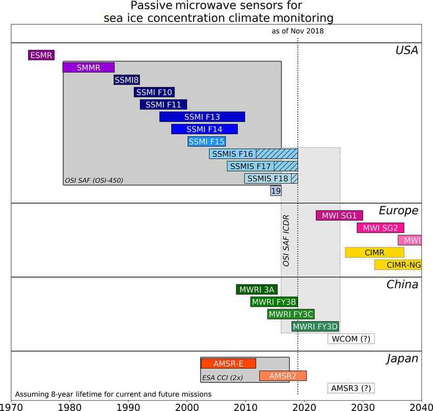
52                                        T. Lavergne et al.: Version 2 of the EUMETSAT OSI SAF and ESA CCI SIC CDRs

Table 2. Platform, instrument, and time period for input brightness temperatures used in the sea-ice data records. All frequencies listed have
both horizontal and vertical polarization channels.

  Platform and   Start date           Stop date           Frequency, in GHz, (footprint    Polar obser-   View angle   Comment
  instrument                                              resolution in km) of channels    vation hole
                                                                                           (north- and
                                                                                           southward)
  Nimbus-7       1 January 1979       20 August 1987      18.0 (54 × 35), 37.0 (28 × 18)   84◦            50.2◦        Operates every other
  SMMR                                                                                                                 day. Two long pe-
                                                                                                                       riods with missing
                                                                                                                       data are 29 March
                                                                                                                       –23 June 1986 and 3
                                                                                                                       –15 January 1987.
  DMSP F08       9 July 1987          18 December 1991    19.3 (70 × 45), 37.0 (38 × 30)   87◦            53.1◦        A long period with
  SSM/I                                                                                                                missing data is 3–
                                                                                                                       31 December 1987.
  DMSP F10       7 January 1991       13 November 1997    19.3 (70 × 45), 37.0 (38 × 30)   87◦            53.1◦        Significant variation
  SSM/I                                                                                                                (slow oscillation) of
                                                                                                                       the incidence angle
                                                                                                                       during its lifetime.
  DMSP F11       1 January 1992       31 December 1999    19.3 (70 × 45), 37.0 (38 × 30)   87◦            53.1◦
  SSM/I
  DMSP F13       3 May 1995           31 December 2008    19.3 (70 × 45), 37.0 (38 × 30)   87◦            53.1◦        F13 operated longer
  SSM/I                                                                                                                but 31 Decem-
                                                                                                                       ber 2008 is the
                                                                                                                       end of coverage in
                                                                                                                       CM-SAF FCDR R3
  DMSP F14       7 May 1997           23 August 2008      19.3 (70 × 45), 37.0 (38 × 30)   87◦            53.1◦
  SSM/I
  DMSP F15       28 February 2000     31 July 2006        19.3 (70 × 45), 37.0 (38 × 30)   87◦            53.1◦        F15 operated longer
  SSM/I                                                                                                                but 31 July 2006 is
                                                                                                                       the end of coverage
                                                                                                                       in CM-SAF FCD
                                                                                                                       R R3
  DMSP F16       1 November 2005      31 December 2015    19.3 (70 × 45), 37.0 (38 × 30)   89◦            53.1◦
  SSMIS
  DMSP F17       14 December 2006     31 December 2015    19.3 (70 × 45), 37.0 (38 × 30)   89◦            53.1◦        F17 operated longer
  SSMIS                                                                                                                but 31 Decem-
                                                                                                                       ber 2015 is the
                                                                                                                       end of coverage in
                                                                                                                       CM-SAF FCDR R3
  DMSP F18       8 March 2010         31 December 2015    19.3 (70 × 45), 37.0 (38 × 30)   89◦            53.1◦        F18 operated longer
  SSMIS                                                                                                                but 31 Decem-
                                                                                                                       ber 2015 is the
                                                                                                                       end of coverage in
                                                                                                                       CM-SAF FCDR R3
  EOS Aqua       1 June 2002          3 October 2010      6.9 (75 × 43), 18.7 (27 × 16),   89.5◦          55◦
  AMSR-E                                                  36.5 (14 × 9)
  GCOM W1        23 July 2012         31 May 2017         6.9 (62 × 35), 18.7 (22 × 14),   89.5◦          55◦          AMSR2 operated
  AMSR2                                                   36.5 (12 × 7)                                                longer but 31 May
                                                                                                                       2017 is the last date
                                                                                                                       we fetched from
                                                                                                                       JAXA for the CDRs.

The Cryosphere, 13, 49–78, 2019                                                                    www.the-cryosphere.net/13/49/2019/
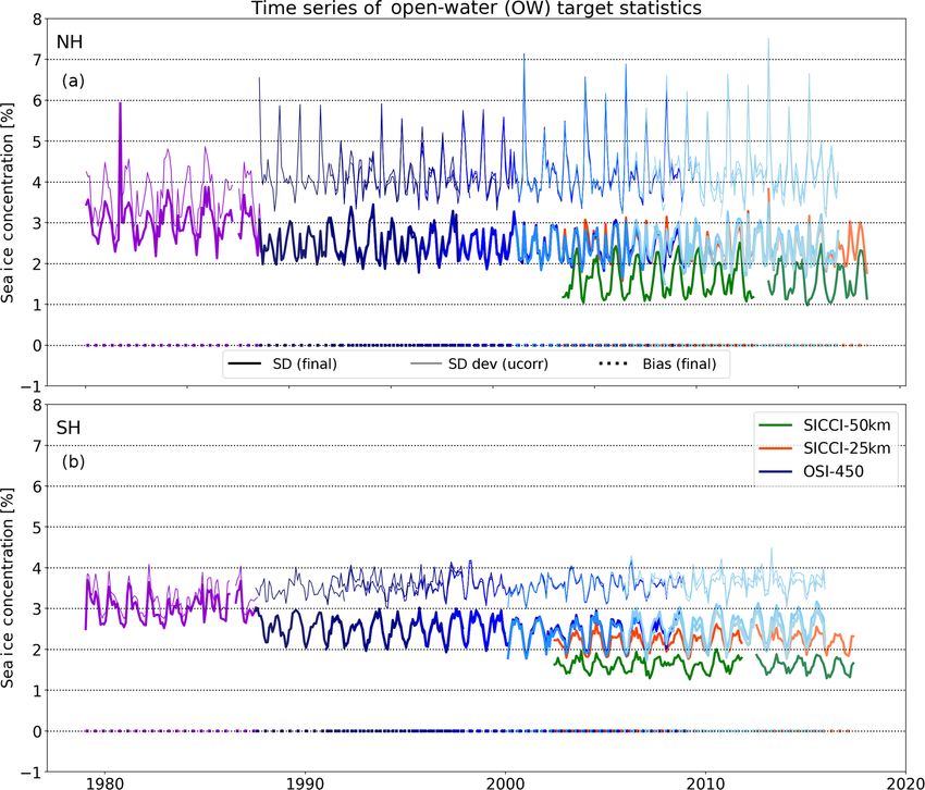
T. Lavergne et al.: Version 2 of the EUMETSAT OSI SAF and ESA CCI SIC CDRs                                                              53

Figure 1. Time-coverage diagram for the new ESA CCI and EUMETSAT OSISAF SIC CDRs. The ESA CCI CDR is based on medium-
resolution AMSR-E and AMSR2 sensors, while the EUMETSAT OSISAF CDR uses the coarse-resolution SMMR, SSM/I, and SSMIS
instruments. Other current and future passive microwave instruments, as well as the OSI SAF ICDRs, are discussed in our Outlook, Sect. 5.2.

pixel. This is because the iFoV takes into account neither              computed from Antenna Temperatures (TA ), screened and
the motion of the antenna (scan direction) nor the motion               corrected for known artefacts like solar intrusion, and in-
of the spacecraft (along its orbit) during the integration pe-          tercalibrated between missions. The AMSR-E data we use
riod needed to acquire a single pixel. The effective field-of-          are the NSIDC FCDR AE_L2A V003 FCDR by Ashcroft
view (eFoV) diameter includes the two effects and is a bet-             and Wentz (2013), covering the full lifetime of the mission
ter measure of the true footprint of the instrument. For ex-            from 1 June 2002 to 4 October 2011. For AMSR2, we use
ample, the eFoV of the SSM/I 19 GHz channels is closer to               recalibrated (version 2) L1R data that we accessed directly
70 × 75 km. The dimensions of the iFoV and eFoV are re-                 from the Japan Aerospace Exploration Agency (JAXA), cov-
ferred to as the resolution of the channels. The sampling is            ering 23 July 2012 until 15 May 2017, that is the end of the
how close in space the FoVs are acquired. Most channels are             SICCI-25km and SICCI-50km CDRs. For both AMSR-E and
thus oversampled.                                                       AMSR2, the TB are available both at their nominal resolution
   Two of the differences between the instrument series are             (documented in Table 2), and post-processed at lower resolu-
the width of their observation swaths, and the inclination of           tion matching those of other channels (e.g. the 36.5 GHz TB
their orbits. This translates into different extents of the polar       at the resolution of the 6.9 GHz channel). We use the nomi-
observation hole, and no data are available for sea-ice moni-           nal resolution of the TB , not the resolution-matched ones. It
toring north of 84◦ (SMMR), 87◦ (SSM/I), 89◦ (SSMIS), and               is noteworthy that the AMSR2 data are not from an FCDR,
89.5◦ (AMSR-E and AMSR2).                                               but rather from an archive of an operational data stream. We
   For our data records, a newly reprocessed version of the             use the data as they are provided by JAXA, without applying
SMMR, SSM/I, and SSMIS data into a Fundamental Cli-                     extra calibration towards AMSR-E (thus unlike Meier and
mate Data Record (FCDR, L1) was accessed from the EU-                   Ivanoff, 2017) since our algorithms do not require such strin-
METSAT Climate Monitoring Satellite Application Facility                gent calibration thanks to using dynamic tuning (Sect. 3.3).
(CM-SAF, Fennig et al., 2017). In the FCDR, the TB are re-

www.the-cryosphere.net/13/49/2019/                                                                  The Cryosphere, 13, 49–78, 2019
54 T. Lavergne et al.: Version 2 of the EUMETSAT OSI SAF and ESA CCI SIC CDRs
2.2 ERA-Interim data The next subsections are devoted to giving some more de-
tails about the main features of the several algorithms in-
The microwave radiation emitted by the ocean and sea ice volved.
travels through the Earth’s atmosphere before being recorded
by the satellite sensors. Scattering, reflection, and emission in 3.2 A hybrid, self-tuning, self-optimizing sea-ice
the atmosphere add or subtract contributions to the radiated concentration algorithm
signal, and challenge our ability to accurately quantify sea-
ice concentration. An initial step in our processing is thus the A new sea-ice concentration algorithm was developed dur-
explicit correction of the TBs for the atmospheric contribu- ing the ESA CCI Sea Ice projects and is used for the three
tion to the top of the atmosphere radiation (see Sect. 3.4.1). CDRs. It is an evolution of the algorithms used in Tonboe
For this purpose, we accessed the global 3-hourly fields from et al. (2016). In this section, we describe both how the algo-
ECMWF’s ERA-Interim reanalysis (Dee et al., 2011). Fields rithm is trained to TB training data sets, and how it is then
of 10 m wind speed, 2 m air temperature, and total column applied to actual TB measurements recorded by satellite sen-
water vapour are used. The ERA-Interim reanalysis starts in sors. The process of selecting training TB data is covered in
January 1979 and is available throughout the time period of Sect. 3.3.
our CDRs. Unavailability of ERA-Interim data prior to 1979 We call the SIC algorithm a hybrid algorithm because it
made it impractical to use the earliest period of SMMR data combines two other SIC algorithms: one that is tuned to per-
(October to December 1978). form better over open-water and low-concentration condi-
tions (named BOW for best open water), and one that is tuned
to perform better over closed-ice and high-concentration con-
3 Algorithms and processing details ditions (named BCI for best closed ice). The combination
equation is quite simply a linear weighted average of BOW
This section introduces the algorithms and some processing and BCI results, where wow is the open-water weight and SIC
elements that are used in the making of the SIC CDRs. In is expressed as sea-ice fraction [0; 1]:
many cases, these algorithms are evolutions of those already
applied in the previous version of the EUMETSAT OSI SAF w = 1; for BOW < 0.7
OW
CDR (OSI-409, Tonboe et al., 2016). wOW = 0; for BOW > 0.9 ;
wOW = 1 − B OW − 0.7
for BOW ∈ [0.7; 0.9]
3.1 Overview of the processing chain 0.2
SIChybrid = wOW × BOW + (1 − wOW ) × BCI . (1)
Figure 2 gives an overview of the processing chain for the
three CDRs. The red boxes are data (stored in data files) OSI-409 already used a hybrid method. It combined the
and the blue boxes are processing elements that apply al- bootstrap frequency mode (BFM) algorithm (Comiso, 1986)
gorithms to the data. The whole process is structured into as BOW , and the Bristol (BRI) algorithm (Smith and Bar-
three chains, at Level 2 (left-hand side), Level 3 (middle), rett, 1994; Smith, 1996) as BCI . Andersen et al. (2007) and
and Level 4 (right-hand side). The input Level 1 (L1) data later Ivanova et al. (2015) confirmed that BFM (BRI) was
files hold the fields observed by the satellite sensors at the so far the published algorithm, including NASA-Team and
top of the atmosphere, in satellite projection: the brightness bootstrap, performing best at low (high) SIC conditions,
temperatures (TB ) are structured in swath files. The Level 2 and notably that BRI is more accurate at high concentration
(L2) chain transforms these into the environmental variables than the bootstrap polarization mode (BPM) algorithm. BFM
of interest, but still on swath projection: the SIC, its associ- and BPM are widely used for sea-ice monitoring in what is
ated uncertainties, and flags. The L2 chain holds an iteration commonly known as the bootstrap algorithm (Comiso and
(marked by the “2nd iteration” grey box) similar to the work- Nishio, 2008). Smith (1996) introduces the BRI algorithm
flow in Tonboe et al. (2016) and stemming from the develop- as a generalization of the BFM and BPM algorithms. BFM
ments of Andersen et al. (2006). This iteration implements computes SIC values in the (19V , 37V ) TB space and BPM
two key correction schemes: the atmospheric correction al- in the (37V , 37H ) TB space. BRI uses the three-dimensional
gorithm at low-concentration range (Sect. 3.4.1) and a novel (19V , 37V , 37H ) TB space, where 19V (19H ) is notation for
correction for systematic errors at high-concentration range “the channel with a frequency near 19 GHz and with vertical
(Sect. 3.4.3). The Level 3 (L3) chain collects the L2 data files (horizontal) polarization”.
and produces daily composited fields of SIC, uncertainties, Figure 3 illustrates the functioning of the BFM algo-
and flags on regularly spaced polar grids. These fields can rithm. Comiso (1986) recognized that the typical signature
and will typically exhibit data gaps, e.g. in case of missing of open-water (OW, SIC = 0 %, grey triangles) TB data clus-
satellite data. The Level 4 (L4) chain fills the gaps, applies ters around an averaged point location (the OW tie point,
extra corrections, and formats the data files that will appear H) in the (19V , 37V ) TB space. Conversely, the closed-ice
in the CDR. (CI, SIC = 100 %, grey discs) TB data mostly cluster along
a line (the consolidated ice line A–D). Comiso (1986) thus
The Cryosphere, 13, 49–78, 2019 www.the-cryosphere.net/13/49/2019/
T. Lavergne et al.: Version 2 of the EUMETSAT OSI SAF and ESA CCI SIC CDRs                                                                     55

Figure 2. From (a) to (c), the three main elements (Level 2, Level 3, and Level 4) in the sea-ice concentration (SIC) processing workflow. The
red boxes depict data files, the blue boxes correspond to individual steps (a.k.a. algorithms) in the processing. The files that exit a processing
chain (e.g. the “L2 SIC and uncert and OWF” at the bottom of the Level 2 processing chain) are the input for the next level of processing.
Acronyms: NT is the Nasa Team algorithm, OWF is open-water filter, RTM is radiative transfer model, uncert stands for uncertainty, L2 is
Level 2, L3 is Level 3, L4 and is Level 4.

designed a SIC algorithm wherein isolines of constant SIC                  A) and the open-water point H. Because this particular plane
are parallel to the A–D line and pass through the measured                 offers the largest dynamic range between the closed-ice and
TB at point P. A geometric algorithm using the intersection                open-water signatures, Smith (1996) states that it is an opti-
of the (H, P) and (A, D) lines at point I returns the SIC value            mum projection plane. This, however, fails to recognize that
(in our example SIC = 68 %). In the same study, similar ag-                the scatter of the closed-ice points around the line and that
gregation of typical TB signatures and a geometric algorithm               of open-water TB samples around the point H are anisotropic
were also used in the (37V , 37H ) TB space (BPM algorithm).               in the (19V , 37V , 37H ) TB space. The open-water scatter
For easing later discussion, here we note that in winter Arc-              has increased variance along the directions resulting from
tic conditions, the typical multi-year sea-ice signature is to             weather effects (including wind speed, cloud liquid water,
the left of the ice line – close to D – while first-year sea               and water vapour) on the emissivity of water. The closed-ice
ice and young sea ice is to the right – closer to A (Comiso,               scatter also has increased variance directions, e.g. due to ice-
2012). The AMSR-E TB samples in Fig. 3 are from Peder-                     type and snow characteristics. Because of these anisotropies,
sen et al. (2018), the ESA CCI Sea Ice Round Robin Data                    the optimal projection plan will generally not be that of BRI.
Package (RRDP).                                                               Our new algorithm is a generalization of BRI. Its principle
   The left-hand panel of Fig. 4 is from Smith (1996) and                  is also introduced in Fig. 4 (left panel). Like in BRI we seek
modified with colours to describe how BFM (frequency                       an optimum “data plane” on which to project the TB data,
scheme), BPM (polarization scheme) and BRI (Bristol algo-                  and we impose that this plane holds the closed-ice line (the
rithm) view the open-water (scatter around H) and closed-ice               D–A line, supported by unit vector u). Vector u is computed
(scatter along the D–A line) data in the three-dimensional                 by principal component analysis (PCA) and is the direction
(19V , 37V , 37H ) TB space. The view direction of BRI is                  with highest variance in the CI TB samples. Conversely to
equivalent to projecting the TB data on a data plane, which                BRI, we do not impose H on the projection plane. We rather
Smith (1996) chose to contain both the closed-ice line (D–                 rotate the plane around u and seek the optimum rotation an-

www.the-cryosphere.net/13/49/2019/                                                                       The Cryosphere, 13, 49–78, 2019
56                                          T. Lavergne et al.: Version 2 of the EUMETSAT OSI SAF and ESA CCI SIC CDRs

                                                                          and confirms the strategy already adopted by Comiso (1986),
                                                                          Andersen et al. (2007), and Tonboe et al. (2016) to construct
                                                                          hybrid algorithms.
                                                                             Figure 4 (right panel) also shows that the optimum rotation
                                                                          angle for OW cases is generally not exactly at θ = 0◦ (BFM).
                                                                          Likewise, the optimum rotation angle for CI cases is gener-
                                                                          ally not the same as that corresponding to the BRI plane. θOW
                                                                          (blue disc) and θCI (red disc) thus indeed define more accu-
                                                                          rate algorithms than BFM and BRI. In that particular exam-
                                                                          ple, the improvement is mostly for OW conditions and lim-
                                                                          ited for CI conditions. The values of θOW and θCI will vary
                                                                          with the exact frequencies, calibration, or viewing angle of
                                                                          the instrument (Table 2), as well as with the OW and CI sig-
                                                                          natures that exhibit regional, seasonal, and interannual varia-
                                                                          tions. The new hybrid, self-optimizing algorithms described
                                                                          in this section can always be tuned to available training data
                                                                          (see Sect. 3.3) and deliver optimum and time-consistent per-
                                                                          formance.
                                                                             We can draw some additional information from the right-
                                                                          hand panel of Fig. 4. First, we seem to confirm the findings of
                                                                          Smith (1996) that BRI performs better than BPM (that corre-
Figure 3. Illustration of the bootstrap frequency mode (BFM,              sponds to θ = +90◦ ). Indeed, the red curve increases all the
Sect. 3.2) and open-water filter (OWF, Sect. 3.4.2) algorithms in a       way to θ = +90◦ and shows poor algorithm accuracy for the
36.5V (x axis) and 18.7 GHz (y axis) TB space of AMSR-E (Winter           (37V , 37H ) projection plane. Second, we observe that both
NH conditions). The grey symbols are actual AMSR-E TB measure-            the blue and red curves hit a maximum standard deviation
ments over SIC = 0 % (triangles) and SIC = 100 % (disks) condi-           (minimum accuracy) somewhere around θ = −60◦ (the peak
tions, from Pedersen et al. (2018). The SIC = 100 % measurements          value is outside the y range of the plot). This quite simply
fall generally along a line (the consolidated ice line), while the mean   corresponds to the worst possible choice of projection plane,
open-water signature is point H. An example measurement P (black
                                                                          for which the OW TB data are projected onto the CI ice line,
circle) falling on the SIC = 68 % isoline illustrates the functioning
of BFM. The blue solid and dotted lines illustrate the tuning and
                                                                          resulting in the smallest dynamic range between OW and CI
functioning of the OWF (as described in Sect. 3.4.2). The black           signatures.
solid curve fitting SIC = 100 % conditions illustrates the ice curve         The geometric descriptions above were all carried out in a
correction (as described in Sect. 3.4.3).                                 (19V , 37V , 37H ) space. The same reasoning can, however,
                                                                          be carried within other 3-D TB spaces, as long as such spaces
                                                                          offer a clustering of the CI conditions along an ice line and
gle θ that yields best SIC accuracy. On Fig. 4 (left panel), we           sufficient dynamic range between the OW signature and the
mark three unit vectors v, corresponding to three different               CI line. In the new CDRs, we use two different TB spaces: the
rotation angles and thus projection planes. By convention,                OSI-450 and SICCI-25km CDRs use the (19V , 37V , 37H )
θ = 0◦ defines the BFM (19V , 37V ) plane, and θ = +90◦                   space, while the SICCI-50km CDR uses the (6V , 37V , 37H )
defines the BPM (37V , 37H ) plane. The BRI plane typi-                   space. Both TB spaces feature two higher-frequency channels
cal has values around θ = +30◦ . By varying θ the optimiza-               with same wavelength but alternate polarization (37 GHz in
tion process samples several planes and eventually returns                both cases), and a lower-frequency vertically polarized chan-
the optimal angles θOW and θCI that respectively define the               nel (19V or 6V ). The role of the higher frequencies is to en-
BOW and BCI algorithms. This optimization step allows us to               sure a significant spread of the CI TB samples along the ice
cope with the anisotropy of the OW and CI TB samples in the               line and thus offer a good base for computing vector u with
(19V , 37V , 37H ) TB space. The right-hand panel of Fig. 4               PCA. They also bring a higher spatial resolution to the re-
shows the process of such an optimization in a case using                 trieved SIC, since higher-frequency channels achieve higher
AMSR2 data from the Northern Hemisphere. The solid lines                  spatial resolution (Table 2). The role of the lower vertically
plot the variation in the accuracy (measured as standard devi-            polarized channel is to ensure a sufficient dynamic range be-
ation of SIC, on the y axis) of the SIC algorithms defined by             tween OW and CI signatures and thus aim to reduce retrieval
the rotation angle (x axis) against the OW (blue) and CI (red)            noise. This is at the cost of bringing a coarser spatial resolu-
training TB data. The minimum of the blue and red curves                  tion into the algorithm.
are not achieved at the same angle. This is a clear illustration             This section has so far covered how the new algorithms are
that there cannot be a single SIC algorithm that performs best            designed and tuned to training data. At the end of the tuning
both on low-concentration and high-concentration conditions               process, the unit vector u defining the closed-ice line, the two

The Cryosphere, 13, 49–78, 2019                                                                  www.the-cryosphere.net/13/49/2019/
T. Lavergne et al.: Version 2 of the EUMETSAT OSI SAF and ESA CCI SIC CDRs 57
Figure 4. (a) Three-dimensional diagram of open-water (H) and closed-ice (ice line between D and A) brightness temperatures in a 19V ,
37V , 37H space (black dots). The original figure is from Smith (1996). The direction U (violet, sustained by unit vector u defined in
Sect. 3.4.3) is shown, and vectors v Bristol (blue), v Best-ice (red), and v Best-OW (green) are added, as well as an illustration of the optimization
of the direction of V for the dynamic (self-optimizing) algorithms. (b) Evolution of the SIC algorithm accuracy for open-water (blue) and
closed-ice (red) training samples as a function of the rotation angle θ in the range [−90◦ ; 90◦ ]. Square symbols are used for the BFM
(frequency mode) and BRI (Bristol) algorithms. Disk symbols locate the new, self-optimizing algorithms.
angles θOW and θCI , and the TB coordinates of the OW and tween different FCDRs, (c) cope with slightly different fre-
CI mean tie points are recorded and stored to disk for later quencies between different instruments (e.g. SMMR, SSM/I,
use. These values are the tuned parameters needed to apply and AMSR-E all have a different frequency around 19 and
the algorithms. Applying the algorithm to a set of new TB 37 GHz; see Table 2), (d) mitigate sensor drift (if not already
data (e.g. a new swath of instrument data) is then straight- mitigated in the FCDR), (e) compensate for trends poten-
forward. Each TB triplet – (19V , 37V , 37H ) or (6V , 37V , tially arising from the use of NWP reanalysed data to correct
37H ) – is projected onto the two optimal planes (defined the TB (see Sect. 3.4.1).
by u and each of the θ angles), and a BFM-like geometric As in Tonboe et al. (2016), the CI training sample is based
SIC algorithm is applied in both planes (like in Fig. 3 but the on the results of the NASA Team (NT) algorithm (Cavalieri
x axis and y axis are now along directions in the projection et al., 1984): locations for which the NT value is greater
plane), yielding two values: SICBOW and SICBCI . The two than 95 % are used as a representation of 100 % ice (Kwok,
SIC values are combined using Eq. (1) to yield the final SIC 2002). Recent investigations, e.g. during the ESA CCI Sea
estimate. Ice projects, confirmed that NT was an acceptable choice for
the purpose of selecting closed-ice samples. The tie points
3.3 Dynamical tuning of the SIC algorithm for applying the NT algorithm to SMMR, SSM/I, and SS-
MIS are taken from Appendix A in Ivanova et al. (2015).
As described in the previous section, tuning the algorithms The same tie points are used for AMSR2 (not covered by
requires two sets of training data: one from OW areas Ivanova et al., 2015) as for AMSR-E. To ensure temporal
(SIC = 0 %) and one from areas we assume have fully CI consistency between the SMMR and later instruments, the
cover (SIC = 100 %). As in Tonboe et al. (2016), the train- closed-ice samples for NH are only used for algorithm tun-
ing of the algorithms is performed separately for each instru- ing if their latitude is less than 84◦ N, which is the limit of
ment and for each hemisphere. In addition, the training is up- the SMMR polar observation hole (Table 2).
dated for every day of the data record and is based on a [−7; The selection of the OW tie-point samples has been re-
+7 days] sliding window worth of daily samples (where Ton- vised since Tonboe et al. (2016), which used fixed ocean
boe et al., 2016 used a [−15; +15 days] sliding window). Our areas at middle to high latitudes. The training areas now
sliding window is made shorter so that tie points react more vary on a monthly basis, and follow the sea-ice cover more
rapidly to seasonal cycles, e.g. onset of melting. closely. In practice, the OW locations are those falling in a
The dynamic training of our algorithms allows us to 150 km wide belt just outside the monthly varying maximum
(a) adapt to interseasonal and interannual variations of the ice extent climatology (which is itself described in Sect. 3.6).
sea-ice and open-water emissivity, (b) cope with differ-
ent calibration of different instruments in a series, or be-
www.the-cryosphere.net/13/49/2019/ The Cryosphere, 13, 49–78, 201958 T. Lavergne et al.: Version 2 of the EUMETSAT OSI SAF and ESA CCI SIC CDRs
3.4 Strategies to further reduce systematic errors and servation.
random noise
TBnwp = F Wnwp , Vnwp , Lnwp = 0; TS , SICucorr , θ0
TBref = F (0, 0, 0; TS , SICucorr , θinstr )
The algorithms described in Sect. 3.2 are self-optimizing δTB = TBnwp − TBref
so that they yield the highest accuracy at high- and low-
concentration ranges. Nevertheless, all TB triplets with a de- TBcorr = TB − δTB (2)
parture from the mean CI or OW signatures will yield a
For TBnwp , the RTM function F simulates the brightness
departure from 0 % and 100 % sea-ice concentration. Ran-
temperature emitted at view angle θ0 by a partially ice-
dom departures that do not have apparent spatial or tem-
covered scene with sea-ice concentration SIC, and with sur-
poral structures are often referred to as “random noise”,
face and atmospheric states described by Wnwp (10 m wind
while departures that are somewhat stable (correlated) in
speed, m s−1 ), Vnwp (total columnar water vapour, mm),
space and time are referred to as “systematic errors”. Anal-
Lnwp (total columnar liquid water content, mm), and TS
ysis of time series of sea-ice concentration maps retrieved
(2 m air temperature). θinstr is the nominal incidence angle
from the algorithm from Sect. 3.2 reveal that the departure
of the instrument series (see Table 2). Our double-difference
at low-concentration range (open water) is typically random
scheme is thus both a correction for the atmosphere influence
noise, while more systematic errors are observed at high-
on the TB (as predicted by the NWP fields) and a correction to
concentration range (closed ice). This is explained by the
a nominal incidence angle. The latter is required to stabilize
different nature of the error sources playing a role at these
the DMSP SSM/I F10 signal, the view angle of which varied
two ends of the sea-ice concentration range: weather-related
significantly: the peak-to-peak daily average incidence angle
effects at synoptic scales over open water, and surface emis-
variation due to the platform’s orbital drift was 52.6–53.7◦
sivity variability (due to ice type, temperature of the emission
according to Colton and Poe (1999). The typical values of
layer, snow depth, etc.) over closed ice. In this section, we
δTB range from about 10 K over open water to few tenths of
describe strategies implemented in the processing chain to
a kelvin over consolidated sea-ice. The liquid water content
further reduce random noise over open water, and systematic
(L) fields from global NWP fields (and ERA-Interim in par-
errors over closed ice. Both correction steps are applied dur-
ticular) were found to not be accurate enough to be used in
ing the second iteration of the L2 chain (Fig. 2) and we note
our atmospheric correction scheme (Lu et al., 2018). The TB
SICucorr (uncorrected), the uncorrected SIC value, before the
are thus not corrected for L (L = 0 in both TBnwp and TBref ),
start of the second iteration.
and the induced remaining noise transfers into uncertainty in
SIC.
We use the remote sensing systems (RSSs) RTM, for
3.4.1 Radiative transfer modelling for correcting which the tuning to different instruments is documented in
atmosphere influence on brightness temperatures Wentz (1983) for SMMR, Wentz (1997) for SSM/I and SS-
MIS, and Wentz and Meissner (2000) for AMSR-E and
AMSR2. It is a parameterized, fast RTM optimized for the
As described in Andersen et al. (2006) and confirmed in frequencies and view angles covered by the passive mi-
Ivanova et al. (2015), the accuracy of retrieved sea-ice con- crowave sensors at hand. It originally allowed ocean and at-
centration can be greatly improved when the brightness tem- mosphere simulations and was later extended to cover sea-ice
peratures are corrected for atmospheric contribution by us- surface conditions (Andersen et al., 2006). Since the RTM
ing a radiative transfer model (RTM) combined with surface is used in the double-difference scheme described above,
and atmosphere fields from NWP reanalyses. The correction accurate calibration of the RTM simulation with the mea-
using NWP data is only possible in combination with a dy- sured brightness temperatures is not critical since such off-
namical tuning of the tie points, so that trends from the NWP sets cancel out. The atmospheric correction step has more
model are not introduced into the sea-ice concentration data impact over open-water and low-concentration values than
set. The correction scheme implemented in the new CDRs is over closed-ice conditions. This is because of (1) a generally
based on a double-difference scheme, similar (but not identi- drier atmosphere above the consolidated ice pack, (2) the ef-
cal) to that described in Andersen et al. (2006) or Tonboe et fect of wind speed on ocean (and not sea-ice) emissivity, and
al. (2016). (3) the low emissivity and high reflectivity of water at the fre-
The scheme evaluates the correction offsets δTB (one per quencies we use in SIC algorithms (Andersen et al., 2006).
channel), the difference between two runs of the RTM: TBnwp
uses estimates from NWP fields (in our case ERA-Interim), 3.4.2 Open-water filtering
while TBref uses a reference atmospheric state with the same
air temperature as TBnwp , but zero wind, zero water vapour, The weather filters (WFs) of Cavalieri et al. (1992) have been
and zero cloud liquid water. δTB is thus an estimate of the used in basically all available SIC CDRs except the earlier
atmospheric contribution at the time and location of the ob- EUMETSAT OSI SAF data sets (Andersen et al., 2007; Ton-
The Cryosphere, 13, 49–78, 2019 www.the-cryosphere.net/13/49/2019/T. Lavergne et al.: Version 2 of the EUMETSAT OSI SAF and ESA CCI SIC CDRs 59
boe et al., 2016). WFs are algorithms that combine TB chan- TB data falling below the GR3719v isoline will result in
nels to detect when rather large SIC values (sometimes up GR3719v > T and will thus be flagged as OW (SIC = 0 %)
to 50 % SIC) are in fact noise due to atmospheric influence by the GR3719v test. Most of the OW TB data (grey tri-
(mainly wind, water vapour, cloud liquid water effects) and angle symbols) are thus flagged as OW, as expected. Some
should be reported as open water (SIC = 0 %). The concept low-concentration TB data (not shown, but falling between H
of WFs is very different from the atmospheric correction of and (A–D), closer to H) will also be detected as OW by the
TB described in the previous section: the atmospheric correc- GR3719v test. This is an illustration of how WFs based on
tion reduces noise in the resulting SIC fields (but does not this gradient ratio will not only successfully detect false sea
yield exactly SIC = 0 % over open water), while the WF is ice as open water, but also wrongly result in ice-free condi-
a binary test that decides whether a pixel should be set to tions where some true sea ice should have been observed.
exactly SIC = 0 % or left unaffected. In the new CDRs, we The greediness of the GR3719v filter is controlled by the
combine both approaches as we apply the WFs after the at- threshold T , the tuning of which is of paramount impor-
mospheric correction. tance for the temporal consistency of the climate data record.
While WFs are effective at removing false sea ice in open- The varying signature of sea-ice and ocean emissivity with
water regions, they will always falsely remove (detect as time and hemisphere, the different frequencies of the 19 and
open water) some amount of low-concentration (and/or thin) 37 GHz channels for different instruments, and the varying
sea ice, especially along the ice edge (Ivanova et al., 2015). effects of atmospheric correction all prevent the adoption of
This is why the OSI SAF SIC CDRs have so far not adopted fixed thresholds. Instead, we adopt a dynamic approach to
WFs and why the effect of WFs can be fully reverted in our tune the threshold. Our WF is tuned to avoid removing true
new SIC CDRs on an ad-hoc basis by using status flags in ice with concentration larger than 10 %, on average. The tun-
the product files (see Sect. 4.1). ing is shown in Fig. 3. First, the coordinates for the point
The WF by Cavalieri et al. (1992) detects (and con- J are computed: J falls where the SIC = 10 % isoline (thick
sequently forces SIC to 0 %) all observations with either blue line) crosses the (blue, dotted) line between the OW sig-
GR3719v > 0.050 and/or GR2219v > 0.045 as open water. nature point H and a point at the rightmost end of the line A–
The GR notation stands for gradient ratio and this quantity D. Then, the GR3719v value corresponding to J is computed
is computed, e.g. as GR3719v = (TB37v − TB19v )/(TB37v + and used as a threshold T . Since the exact locations of H, A,
TB19v ). Many investigators have re-used these thresholds un- and D vary for each instrument, hemisphere, and day in the
changed, while they should really be adapted to the different data record, our threshold T will change (although slightly)
wavelengths and calibration of the different instruments. For during the whole data record, without the need for prescribed
example, Spreen et al. (2008) adapted the GR3719v thresh- values (such as T = 0.05 for the Cavalieri, 1992 WF). The
old to 0.045 and GR2219v to 0.040 when processing sea- value of 10 % SIC is chosen to be below the threshold com-
ice concentration with AMSR-E data. The NOAA/NSIDC monly used for defining the sea-ice extent (15 % SIC) to en-
sea ice concentration CDR uses the Cavalieri et al. (1992) sure that the weather filter does not interfere when computing
thresholds, with the exception of Southern Hemisphere pro- the sea-ice extent.
cessing for SSMIS F17, where the GR3719v threshold is set We note finally that the name “weather filter” can be mis-
to 0.053 (Algorithm Theoretical Basis Document for Meier leading as the non-expert could understand that it is meant
et al., 2017). for filtering out weather effects (false sea ice) from calm
Following Lu et al. (2018), we use a WF computed from open-water and low-ice-concentration conditions. As seen in
TB that has been corrected for atmospheric influence and fea- Fig. 3, this is not how the GR3719v filter works, as it will
tures a test for GR3719v only. There are two reasons for not remove true sea ice as well, even in calm weather conditions
using GR2219v: (1) a near 22 GHz channel is not available (OW samples below J). In addition, GR3719v contains in-
throughout the satellite time series (Sect. 2.1); and (2) the formation on sea-ice type (Cavalieri et al., 1984) and it is
correction of water vapour using ERA-Interim data is effec- desirable that the filter should work equally for first-year and
tive enough in polar regions so that very limited additional multi-year sea ice. For these reasons, we refer to such a fil-
screening is triggered by GR2219v when applied after TB ter as an “open-water filter” (OWF) and include a test for the
correction. Indeed, GR2219v is mostly effective at detecting SIC value. The OWF implemented in the new CDRs is thus
water vapour effects, while GR3719v is effective at screening defined by the following two tests (corresponding to the thick
cloud liquid water and wind-roughening effects (Cavalieri et solid blue line in Fig. 3):
al., 1995).
GR3719v ≥ T
The functioning of the WF is illustrated in Fig. 3. In the . (3)
or SIC ≤ 10 %
(19V , 37V ) diagram of Fig. 3, the GR3719v = T isolines
are steeper than the consolidated ice line (A–D). For se- Notably, we compute OWFs in swath projection, in the
lected values of T , the isoline intersects the regions of typ- Level 2 chain (Fig. 2). As a result, each FoV observation at
ical open-water and low-concentration ice (the solid blue Level 2 is attached to a binary flag corresponding to OWF
isoline GR3719v = 0.058 is plotted as an illustration). All detection. This binary flag is combined during gridding and
www.the-cryosphere.net/13/49/2019/ The Cryosphere, 13, 49–78, 201960 T. Lavergne et al.: Version 2 of the EUMETSAT OSI SAF and ESA CCI SIC CDRs
daily averaging to yield Level 3 fields of OWFs. This is a bet- pose. As part of the processing, the consolidated ice curve is
ter approach than computing WFs from daily averaged grid- not used in the two-dimensional BFM space, but in the three-
ded TB data, which will smooth and smear the sea-ice edge dimensional data plane of the dynamic SIC algorithm (see
region, as well as rapidly changing weather effects such as Sect. 3.2). The amplitude of the sea-ice curve around the sea-
cloud liquid water content or wind roughening. Computing ice line can be different in shape in the SIC algorithm plane.
OWFs at Level 2 can also help to mitigate the potential im- In addition, the ice curve in Fig. 3 is fitted through the consol-
pacts of changes in satellite crossing time between different idated ice points from the ESA CCI Sea Ice RRDP (Pedersen
missions. The impact of the dynamic tuning of the OWF is et al., 2018) that spans several years and winter months and
evaluated in Sect. 4.2.1. thus illustrates an average sea-ice curve. The consolidated
sea-ice samples we extract dynamically for [−7; +7 days]
3.4.3 Reducing systematic errors at high-concentration sliding windows (Sect. 3.3) will typically exhibit more vari-
range ability due to shorter-term changes in sea-ice signatures.
Figure 5 (left and middle panels) show the spatial dis-
Wintertime, monthly averaged maps of SICucorr exhibit sys- tribution of the total correction for January 2015 (SIC mi-
tematic errors at high-concentration ranges, which are espe- nus SICucorr ), thus including both the effect of the correc-
cially visible in the central Arctic Ocean. A novel correction tion based on the consolidated ice curve and the effect of the
scheme is implemented as part of the second algorithm iter- RTM-based correction of the TB . Black solid lines show the
ation (Fig. 2) that effectively mitigates most of these system- mean sea-ice edge region (at 15 % and 70 % SIC values) dur-
atic errors over the basin. ing the same period. The left panel shows the average total
By construction, SIC algorithms BFM, BPM, BRI, and correction (daily maps of SIC minus SICucorr averaged over
our new dynamic algorithms consider that the SIC is exactly the month of January 2015), while the centre panel shows the
100 % when the input TB falls on the consolidated ice line effect of the total correction on SIC variability (variability is
(Fig. 3). The concept of an ice line has sustained the devel- the standard deviation of daily SICucorr maps throughout the
opment of SIC algorithms for decades, since it allows al- month minus the same variability of daily SIC maps after
gorithms to return SICs close to 100 % for all consolidated correction).
ice conditions, whatever the type of sea ice (multi-year ice, Over closed-ice conditions (inside the 70 % SIC isoline),
first-year ice, mixture of types). However, careful analysis the regional patterns of the correction are clearly visible
of the spread of consolidated ice samples along the ice line and seem to match variations in sea-ice age: a large posi-
reveals that systematic deviations exist and are stable with tive correction (increased SIC) north of the Canadian Arctic
time. These systematic deviations draw a consolidated sea- Archipelago and Ellesmere Island (intense red colour) where
ice curve, as illustrated with the solid black curve around the the ice is oldest in the Arctic, moderate negative correction
100 % SIC samples. These deviations are best shown in a over a large part of the central basin (extending from the cen-
coordinate system in which abscissae are computed as u.T tral Beaufort Sea, over to the North Pole, and to northern
(dot product of u the unit vector sustaining the consolidated Greenland, light-blue colour, second-year ice), and a slightly
ice line, and T a 3-D TB triplet in TCI , Fig. 4) and the ordi- positive correction again over large parts of the Siberian Arc-
nate as BCI (T ) (the result of the best ice SIC algorithm for a tic (light-red colour, first-year ice). The mean January 2015
given TB triplet). We refer to the quantity u.T as the distance DAL is shown in Fig. 5 (right) (blue, green, and yellow
along the ice line (DAL). Since u points from multi-year ice colours).
to first-year sea ice (Sect. 3.2, and Fig. 4), older ice have On Fig. 5 (right) we observe an overall increase of the
lower DAL values than younger ice. In winter Arctic con- DAL value from the Canadian Arctic Archipelago (multi-
ditions, it is typical to observe that BCI (T ) values are con- year ice) across the pole and towards the Laptev and Kara
sistently lower than 100 % (down to 85 %–90 %) for old ice seas (first-year ice). To confirm the link between DAL and
(low values of DAL) and consistently higher than 100 % (up sea-ice age, we overlay contours ≥ 1 year, ≥ 2 years, and ≥3-
to 105 %–110 %) for new and first-year ice (high values of year-old sea ice for January 2015 from Korosov et al. (2018)
DAL). In between these two extremes, the BCI (T ) values os- on the right panel. Korosov et al. (2018) developed an im-
cillate between being below and over the SIC = 100 % line. proved Lagrangian-based sea-ice age tracking algorithm us-
Our novel correction scheme moves the concept of an ice line ing the sea-ice drift product of the EUMETSAT OSI SAF
to an ice curve that more closely follows the BCI (T ) samples (Lavergne et al., 2010). The correspondence in the transitions
along the u axis. A new ice curve is tabulated for each day in of DAL values with the contour lines of sea-ice age is very
the record by binning the BCI (T ) values by their DAL values. good, indicating that a combination of DAL (right panel) and
This consolidated ice curve defines the SIC 100 % isoline ice curve correction (left panel) could be used for sea-ice type
during the second iteration of Level 2, and – conversely to (if not age) classification studies. This is outside the scope of
the atmospheric correction described in Sect. 3.4.1 – has the our study, which is focused on SIC algorithms and the new
greatest effect on consolidated ice regions. It is noteworthy data records.
that the sea-ice curve shown in Fig. 3 is for illustration pur-
The Cryosphere, 13, 49–78, 2019 www.the-cryosphere.net/13/49/2019/T. Lavergne et al.: Version 2 of the EUMETSAT OSI SAF and ESA CCI SIC CDRs 61
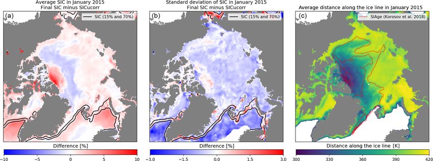
Figure 5. (a, b) Difference maps between the January 2015 mean (a) and temporal variability (b) of the final SIC and the uncorrected SIC
(SICucorr ) in the Arctic Ocean. Black solid lines are at the 15 % and 70 % SIC levels (marginal ice zone). (c) January 2015 mean distance
along the ice line (DAL) values, red lines are transitions between first-year sea ice, second-year sea ice, and older sea ice from Korosov et
al. (2018).
Figure 5 (centre) shows the result of the ice curve cor- enable more accurate retrievals of SICs; thus the ice edge is
rection on SIC variability. In the regions covered with sea- more sharply defined in the daily SIC fields, and this results
ice (> = 70 % SIC), the shades of light blue indicate that in higher variability on a monthly basis.
the variability at high concentration is rather consistently re- In this section, we described the strategies we imple-
duced by about 1 %–2 % SIC by the ice curve correction: mented to improve the accuracy of the SIC algorithms. In the
the SIC after correction is a more accurate description of a next section, we discuss how the remaining noise is quanti-
nearly 100 % ice cover. A limited number of regions show fied and reported to the users of the data records in the form
no improvement (white colour) or slight degradation. This of uncertainties.
reduction in the variability comes in addition to the correc-
tion for the systematic errors (e.g. underestimation north of 3.5 Uncertainties
Canadian Arctic Archipelago; see left panel for which the ice
curve correction was designed). The analysis of the closed- Spatially and temporally varying uncertainty estimates for
ice (> = 70 % SIC) region in Fig. 5 thus confirms that the each and every SIC value are required of state-of-the-art
ice curve correction works as expected at high-concentration CDRs (GCOS-IP, 2016). Uncertainties are needed as soon
range and is potentially linked to the age of sea ice. as the data are compared to other sources (e.g. other simi-
In the open-water regions of Fig. 5 (outside the 15 % SIC lar data records) or when data are assimilated into numerical
contour), the reduction in variability (centre panel) is even models. However, there is no unique way to derive nor to
larger (3 %–4 % SIC) than over closed-ice regions. This re- present uncertainties in EO data (Merchant et al., 2017).
duction is the result of the atmospheric correction step, de- The approach to derive and present uncertainties in the
scribed in Sect. 3.4.1. From the left panel, it appears that the new SIC CDRs is mostly similar to that of Tonboe et
atmospheric correction step on average increases SIC (shades al. (2016): we make the assumption that the total uncertainty
of red) over open-water regions close to the sea-ice edge, e.g. σtot is given by two uncertainty components. That is,
in East Greenland Sea, Barents Sea, and in Labrador Sea. 2
σtot 2
= σalgo 2
+ σsmear , (4)
These regions generally present negative SICs before correc-
tion and are brought closer to 0 % SIC by the process of at- where σalgo is the inherent uncertainty of the SIC algorithm
mospheric correction. This is due to the training OW samples (algorithm uncertainty) including sensor noise and the resid-
being selected in lower-latitude conditions (ocean surface, at- ual geophysical noise quantified as variability around the OW
mosphere conditions) rather than prevailing closer to the ice and CI mean signatures, and σsmear is the representativeness
edge and is also discussed in Sect. 4.2.3 when evaluating un- uncertainty due to resampling from satellite swath to a grid
certainties. (smearing uncertainty) and the mismatch between footprints
Still in Fig. 5 (centre panel), the increased variability (red at different channels.
tones) between the 15 % and 70 % isolines follows logically The derivation of σalgo is to a large extent similar to that
from the two above-mentioned reductions: the corrections described in Tonboe et al. (2016). This term is derived from
www.the-cryosphere.net/13/49/2019/ The Cryosphere, 13, 49–78, 2019You can also read