Development of an optical sensor system for the characterization of Cascadia Basin, Canada - TUM
←
→
Page content transcription
If your browser does not render page correctly, please read the page content below
Development of an optical sensor system for
   the characterization of Cascadia Basin,
                  Canada

                            Andreas Gärtner

Masters thesis
11. December 2018

First Examiner: Prof. Dr. Elisa Resconi
Second Examiner: Prof. Dr. Laura Fabbietti

Technical University of Munich
Department of Physics
Experimental Physics with Cosmic Particles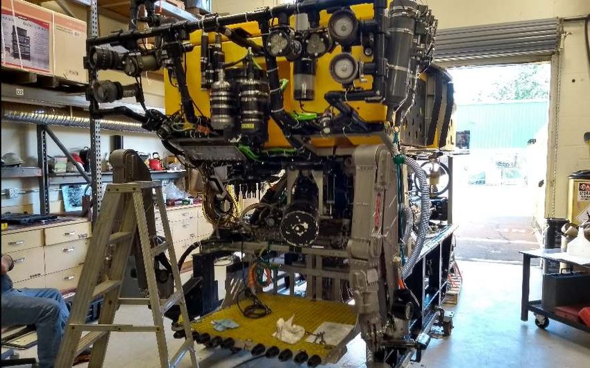
Abstract

  High energy neutrino astronomy uses large volume detectors to search for astrophysical
neutrinos sources. Detectors such as IceCube at the Geographic South Pole instrumented
a cubic kilometer of ice measuring Cherenkov radiation created by neutrino-matter
interactions. Using the clear water of the deep sea as the Cherenkov medium has so
far posed severe difficulties in deploying and maintaining the offshore infrastructure,
although a detector of this type is currently developed by KM3NeT in the Mediterranean.
  Ocean Networks Canada (ONC), an initiative of the University of Victoria, has been
creating and maintaining the longest deep sea infrastructure available for scientific in-
struments, located off the coast of Canada. One of their network nodes, located on the
Pacific abyssal plain of Cascadia Basin, could be in an ideal position for a future neutrino
telescope.
  This thesis concerns the Strings for Absorption Length in Water (STRAW), which have
been developed in 2018 in collaboration with ONC and the University of Alberta. Two
strings with optical modules have been deployed at Cascadia Basin in order to measure
the optical properties of the water and study the feasibility of a larger setup. The primary
measurement goals are absorption, scattering and background radiation.
  In this thesis I will report about the mechanical setup of the two strings and the details
of the deployment mechanism and operation.
Contents

Introduction                                                                                                                                            6

1 Neutrino physics and large volume detectors                                                                                                         8
  1.1 Postulation and discovery . . . . . . . . . . . . . . . . . .                                            .   .   .   .   .   .   .   .   .   . 8
  1.2 Sources . . . . . . . . . . . . . . . . . . . . . . . . . . . . .                                        .   .   .   .   .   .   .   .   .   . 10
  1.3 Neutrino telescopes . . . . . . . . . . . . . . . . . . . . . .                                          .   .   .   .   .   .   .   .   .   . 11
  1.4 Relevant environment parameters for neutrino telescopes                                                  .   .   .   .   .   .   .   .   .   . 13

2 Ocean Networks Canada                                                                                                                                15
  2.1 Overview . . . . . . . . . . . . . . . . . . . . . . . . . . . .                                         .   .   .   .   .   .   .   .   .   .   15
  2.2 Infrastructure and instrument platforms . . . . . . . . . .                                              .   .   .   .   .   .   .   .   .   .   15
  2.3 Deployment method . . . . . . . . . . . . . . . . . . . . .                                              .   .   .   .   .   .   .   .   .   .   17
  2.4 Remotely Operated Platform for Ocean Science (ROPOS)                                                     .   .   .   .   .   .   .   .   .   .   17

3 Simulations and expected environment                                                     20
  3.1 Water transmittivity . . . . . . . . . . . . . . . . . . . . . . . . . . . . . . . . 20
  3.2 The string in the current . . . . . . . . . . . . . . . . . . . . . . . . . . . . . 21
  3.3 Preliminary light simulation . . . . . . . . . . . . . . . . . . . . . . . . . . . 21

4 The double string                                                                                                                                    25

5 Modules                                                                                                                                              27
  5.1 POCAM . . . . . . . . . . .      .   .   .   .   .   .   .   .   .   .   .   .   .   .   .   .   .   .   .   .   .   .   .   .   .   .   .   .   27
      5.1.1 Housing . . . . . .        .   .   .   .   .   .   .   .   .   .   .   .   .   .   .   .   .   .   .   .   .   .   .   .   .   .   .   .   27
      5.1.2 Integrating sphere .       .   .   .   .   .   .   .   .   .   .   .   .   .   .   .   .   .   .   .   .   .   .   .   .   .   .   .   .   27
      5.1.3 In-situ calibration .      .   .   .   .   .   .   .   .   .   .   .   .   .   .   .   .   .   .   .   .   .   .   .   .   .   .   .   .   28
      5.1.4 Electronics . . . . .      .   .   .   .   .   .   .   .   .   .   .   .   .   .   .   .   .   .   .   .   .   .   .   .   .   .   .   .   28
      5.1.5 Kapustinsky circuit        .   .   .   .   .   .   .   .   .   .   .   .   .   .   .   .   .   .   .   .   .   .   .   .   .   .   .   .   29
  5.2 SDOM . . . . . . . . . . . .     .   .   .   .   .   .   .   .   .   .   .   .   .   .   .   .   .   .   .   .   .   .   .   .   .   .   .   .   30
      5.2.1 Housing . . . . . .        .   .   .   .   .   .   .   .   .   .   .   .   .   .   .   .   .   .   .   .   .   .   .   .   .   .   .   .   30
      5.2.2 Photomultiplier . .        .   .   .   .   .   .   .   .   .   .   .   .   .   .   .   .   .   .   .   .   .   .   .   .   .   .   .   .   30
      5.2.3 Electronics . . . . .      .   .   .   .   .   .   .   .   .   .   .   .   .   .   .   .   .   .   .   .   .   .   .   .   .   .   .   .   31
  5.3 The Medusa board . . . . .       .   .   .   .   .   .   .   .   .   .   .   .   .   .   .   .   .   .   .   .   .   .   .   .   .   .   .   .   31

6 Material choice and corrosion protection                                                 34
  6.1 Materials overview . . . . . . . . . . . . . . . . . . . . . . . . . . . . . . . . 34
  6.2 Steel and steel protection . . . . . . . . . . . . . . . . . . . . . . . . . . . . . 34

                                                       3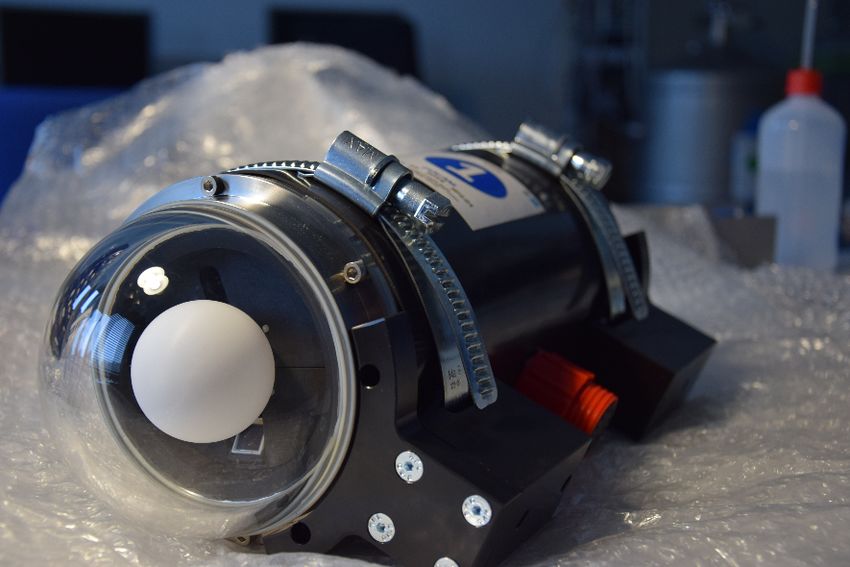
Contents

   6.3    Different metals in contact       .   .   .   .   .   .   .   .   .   .   .   .   .   .   .   .   .   .   .   .   .   .   .   .   .   .   .   .   35
   6.4    Zinc coating . . . . . . . .      .   .   .   .   .   .   .   .   .   .   .   .   .   .   .   .   .   .   .   .   .   .   .   .   .   .   .   .   36
   6.5    Paint . . . . . . . . . . . . .   .   .   .   .   .   .   .   .   .   .   .   .   .   .   .   .   .   .   .   .   .   .   .   .   .   .   .   .   37
   6.6    Bolts and nuts . . . . . . .      .   .   .   .   .   .   .   .   .   .   .   .   .   .   .   .   .   .   .   .   .   .   .   .   .   .   .   .   37
   6.7    Steel wires . . . . . . . . .     .   .   .   .   .   .   .   .   .   .   .   .   .   .   .   .   .   .   .   .   .   .   .   .   .   .   .   .   38
   6.8    Overdesign . . . . . . . . .      .   .   .   .   .   .   .   .   .   .   .   .   .   .   .   .   .   .   .   .   .   .   .   .   .   .   .   .   38
   6.9    Stainless steel corrosion . .     .   .   .   .   .   .   .   .   .   .   .   .   .   .   .   .   .   .   .   .   .   .   .   .   .   .   .   .   38
   6.10   Winch . . . . . . . . . . . .     .   .   .   .   .   .   .   .   .   .   .   .   .   .   .   .   .   .   .   .   .   .   .   .   .   .   .   .   39
   6.11   Choice of colors . . . . . .      .   .   .   .   .   .   .   .   .   .   .   .   .   .   .   .   .   .   .   .   .   .   .   .   .   .   .   .   39
   6.12   Non-metallic components           .   .   .   .   .   .   .   .   .   .   .   .   .   .   .   .   .   .   .   .   .   .   .   .   .   .   .   .   40

7 Construction                                                                                                                                              41
  7.1 Anchor . . . . . . . . . . . . . . . . . . . . . . . . . .                                        .   .   .   .   .   .   .   .   .   .   .   .   .   41
  7.2 Module mountings . . . . . . . . . . . . . . . . . . .                                            .   .   .   .   .   .   .   .   .   .   .   .   .   42
  7.3 Spacers . . . . . . . . . . . . . . . . . . . . . . . . . .                                       .   .   .   .   .   .   .   .   .   .   .   .   .   43
  7.4 Top spacer . . . . . . . . . . . . . . . . . . . . . . . .                                        .   .   .   .   .   .   .   .   .   .   .   .   .   45
  7.5 Compensating anchor tilt . . . . . . . . . . . . . . . .                                          .   .   .   .   .   .   .   .   .   .   .   .   .   46
  7.6 Bottom spacer . . . . . . . . . . . . . . . . . . . . . .                                         .   .   .   .   .   .   .   .   .   .   .   .   .   46
  7.7 Mini junction box mounting . . . . . . . . . . . . . .                                            .   .   .   .   .   .   .   .   .   .   .   .   .   47
  7.8 Markings and nomenclature of strings and modules                                                  .   .   .   .   .   .   .   .   .   .   .   .   .   47
  7.9 Steel wire rope . . . . . . . . . . . . . . . . . . . . . .                                       .   .   .   .   .   .   .   .   .   .   .   .   .   48
  7.10 Data cables . . . . . . . . . . . . . . . . . . . . . . . .                                      .   .   .   .   .   .   .   .   .   .   .   .   .   49
  7.11 Buoyancy . . . . . . . . . . . . . . . . . . . . . . . . .                                       .   .   .   .   .   .   .   .   .   .   .   .   .   50
  7.12 Transport . . . . . . . . . . . . . . . . . . . . . . . . .                                      .   .   .   .   .   .   .   .   .   .   .   .   .   51

8 Calibration and testing                                                                                                                                   53
  8.1 Measuring the data cable length                   .   .   .   .   .   .   .   .   .   .   .   .   .   .   .   .   .   .   .   .   .   .   .   .   .   53
  8.2 Magnetometer . . . . . . . . . .                  .   .   .   .   .   .   .   .   .   .   .   .   .   .   .   .   .   .   .   .   .   .   .   .   .   53
  8.3 Vibration testing . . . . . . . . .               .   .   .   .   .   .   .   .   .   .   .   .   .   .   .   .   .   .   .   .   .   .   .   .   .   55
  8.4 Pressure testing . . . . . . . . .                .   .   .   .   .   .   .   .   .   .   .   .   .   .   .   .   .   .   .   .   .   .   .   .   .   56

9 Designing a winch for string deployment                                                                                                                   59
  9.1 Expected forces and dimensioning .                            .   .   .   .   .   .   .   .   .   .   .   .   .   .   .   .   .   .   .   .   .   .   59
  9.2 Material . . . . . . . . . . . . . . . . .                    .   .   .   .   .   .   .   .   .   .   .   .   .   .   .   .   .   .   .   .   .   .   59
  9.3 Motor . . . . . . . . . . . . . . . . . .                     .   .   .   .   .   .   .   .   .   .   .   .   .   .   .   .   .   .   .   .   .   .   60
  9.4 Axle . . . . . . . . . . . . . . . . . . .                    .   .   .   .   .   .   .   .   .   .   .   .   .   .   .   .   .   .   .   .   .   .   60
  9.5 Wheel . . . . . . . . . . . . . . . . . .                     .   .   .   .   .   .   .   .   .   .   .   .   .   .   .   .   .   .   .   .   .   .   61
  9.6 Frame . . . . . . . . . . . . . . . . . .                     .   .   .   .   .   .   .   .   .   .   .   .   .   .   .   .   .   .   .   .   .   .   62
  9.7 String assembly and spooling . . . .                          .   .   .   .   .   .   .   .   .   .   .   .   .   .   .   .   .   .   .   .   .   .   62

10 Deployment preparation and testing at Ocean Networks Canada                                                                                              69

11 Deployment                                                                                                                                               73

                                                            4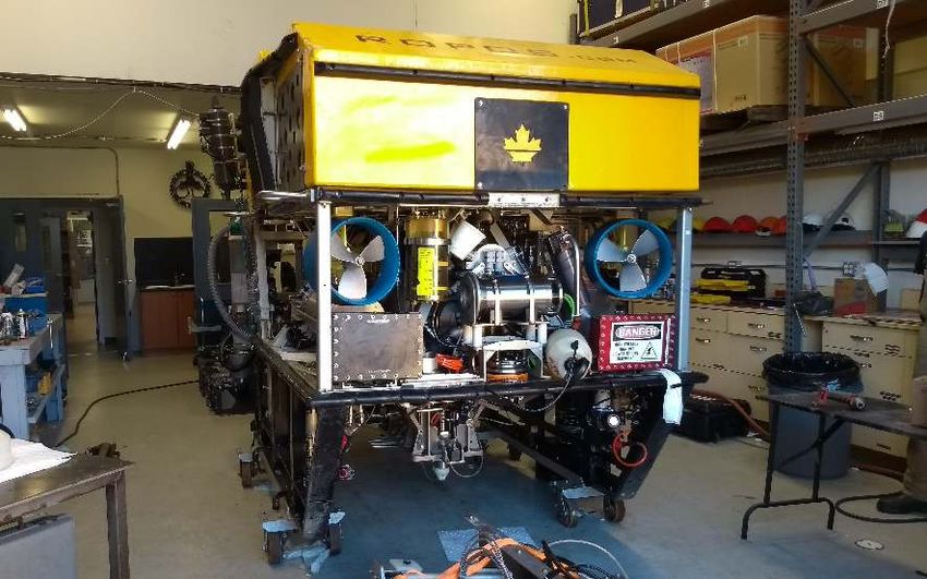
List of abbreviations

 ECP     Experimental Physics with Cosmic Particles, working group of the au-
         thor at TUM
 GVD     Gigaton Volume Detector, neutrino detector in Lake Baikal
 ODI     Brand of underwater cables and connectors from Teledyne
 ONC     Ocean Networks Canada, an initiative of the University of Victoria
 PMT     Photomultiplier tube
 POCAM   Precision Optical Calibration Module, a module creating isotropic
         nanosecond pulses
 RIB     Rigid inflatable boat, a lightweight boat assisting the main vessel during
         deployment
 POM     Polyoxymethylene, hard plastic
 ROPOS   Remotely Operated Platform for Ocean Science, the ROV used during
         deployment
 ROV     Remotely operated underwater vehicle, an unmanned submarine for
         inspection and maintenance of underwater structures
 SDOM    STRAW Digital Optical Module
 STRAW   Strings for Absorption Length in Water
 TUM     Technical University of Munich
 UVIC    University of Victoria
 ZTL     Central Technology Lab of TUM

                                       5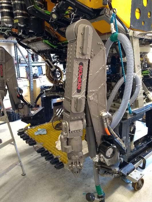
Introduction

  The Strings for Absorption Length in Water (STRAW) setup consists of two double
strings placed at 37 m distance in Cascadia Basin.
  Two types of optical instruments are mounted on the strings. The Precision Optical
Calibration Module (POCAM), a calibration module developed for IceCube and already
tested in GVD provides an isotropic light source creating nanosecond flashes of different
wavelengths. The STRAW Digital Optical Module (SDOM) contains two photomultiplier
tubes, one facing up and one facing down. Five SDOMs and three POCAMs compose
STRAW. We study the absorption and scattering length measuring with the SDOMs the
light emitted by POCAM flashes. When the POCAMs do not flash, the dark rate is
measured, which is influenced by bioluminescence and radioactivity.
  The goal of STRAW is not only to measure water properties, but to also to study the
feasibility of a large neutrino telescope at Cascadia Basin with respect to infrastructure
and deployment capabilities. We therefore chose a setup which mimics a larger detector
as closely as possible, using optical modules and calibration light sources on mooring
lines in the same way as they could be used in a future detector.
  Each string has a buoyancy at the top and an anchor at the bottom. The strings have a
length of 140 m in total with instruments at the heights of 30 m, 50 m, 70 m and 110 m. By
using double strings we prevent the rotation of the modules around the strings, making
sure that the modules of the two strings face each other. The strings were assembled
at TUM, then spooled onto a newly developed winch, tested at ONC, and deployed in
June 2018. Fig. 1 shows a sketch of the two STRAW strings. Four modules per string are
connected to a mini junction box at the bottom, developed by ONC. The strings consist of
two steel wire ropes each, which are kept apart by spacers. The strings are referred to as
string Blue and string Yellow.
  STRAW has started operation in summer 2018 and is currently taking continuous
measurements. So far all modules are fully operational and the intactness of the strings
has been checked twice by a remotely controlled underwater vehicle (ROV).
  The instruments of STRAW will be described only briefly in this thesis, further informa-
tion can be found in the complementary thesis by F. Henningsen [Hen18].

[Hen18] Felix Henningsen. “Optical Characterization of the Deep Pacific Ocean: Development of an Optical
Sensor Array for a Future Neutrino Telescope”. MA thesis. Technical University of Munich, July 2018

                                                   6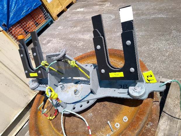
Contents

Figure 1: Overview of the two STRAW strings. Four modules per string are connected to
a mini junction box at the bottom, developed by ONC. Each string consists of two steel
lines, which are kept apart by spacers.

                                          7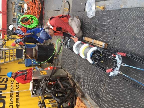
Chapter 1

Neutrino physics and large volume
detectors

  Neutrino astronomy is a relatively new field at the boundaries of particle physics and
astronomy. It aims to detect neutrinos created in astrophysical sources using large neutrino
telescopes, which extend up to one cubic kilometer in volume.

1.1 Postulation and discovery
  In 1930 Wolfgang Pauli suggested the existence of a light uncharged particle, a third
product of the β-decay, to explain the continuous energy spectrum of the decay. Pauli
suggested, that what was before considered a two-body decay (nucleus and electron),
which should have a discrete spectrum, is in fact a three-body decay (nucleus, electron
and neutrino), where the third particle had evaded detection.
  Nowadays this particle, known as neutrino, is an integral part of the Standard Model of
Particle Physics. Each charged lepton (electron, muon, and tauon) has a corresponding
neutral neutrino partner. Neutrinos react only via the weak interaction, which is the
weakest of the three forces in the Standard Model with cross sections of about 10−44 cm.
Unlike the other interactions, the weak interaction can not create bound states and is only
relevant for flavor changes of particles, the most prominent example being the β-decay:

      n → p + e− + ν̄e                                                                             (1.1)

Just as the β-decay creates a (anti-)neutrino, the inverse β-decay can capture a neutrino
and serve for neutrino detection. Due to the small cross section of the weak interaction,
the probability for this process is negligible unless either a high neutrino flux or a high
target volume is used.
  The first detection of neutrinos was done in 1956 by Cowan and Reines [Cow+56] via
the inverse β-decay

      ν̄e + p → e+ + n                                                                             (1.2)

and consecutive reactions in water containing cadmium chloride. For this experiment, a
layered setup of water tanks and scintillation detectors with photomultiplier tubes was
[Cow+56] C.L. Cowan et al. “Detection of the Free Neutrino: a Confirmation”. In: The Theory of Beta-Decay
(1956), pp. 129–135. doi: 10.1016/b978-0-08-006509-0.50008-9

                                                   8
Chapter 1. Neutrino physics and large volume detectors
placed in the strong anti-neutrino flux of a nuclear reactor, looking for the coincidence of
the photons created by the positron annihilation and the neutron capture of the cadmium
ions:
e+ + e− → 2γ (1.3)
113 2+ 114 2+
n+ Cd → Cd +γ (1.4)
Consecutively, muon neutrinos and tau neutrinos were discovered, where the experimen-
tators made explicit use of the low interaction probability and therefore deep penetration
of neutrinos through matter. In 1962, the first artificial neutrino beam was created to
detect muon neutrinos [Dan+62]. A proton beam hitting a beryllium target produced fast
pions. After a short free path, where the pions had time to partially decay into muons and
muon neutrinos, a 14 m steel shield filtered out everything except the neutrinos, which
were detected in a 10 t aluminium spark chamber.
In 2000, the DONUT collaboration detected the first tau neutrinos [Kod+01]. Similar to
the muon neutrino detection, a proton beam hitting a tungsten target produced mesons,
which in turn decayed into a multitude of secondary particles. Using a steel shield
most non-neutrinos were filtered out. In a target consisting of many emulsion sheets
the neutrinos would interact and create secondary particles, whose tracks left marks in
the sheet. Using further detectors to identify secondary and tertiary particles, possible
tau neutrino events were registered. Later, the emulsion layers were photographically
developed and particle tracks were reconstructed. Four tau neutrino events were found,
identifiably by a characteristic track of a tauon starting in the middle of the emulsion
track, without any tracks leading up to it, and having a kink after few millimeters when
the tauon decays.
These early experiments show a fundamental pattern of neutrino detection, the use of a
detector with a large volume to compensate for low statistics, where the detector is placed
after a shield filtering out most other particles.
The first neutrinos from an extraterrestrial source were discovered by the team of R.
Davis Jr. [Cle+98]. Solar neutrinos are created during the proton fusion in the core of the
sun:
p + p → 2 H + e+ + νe (1.5)
In the Homestake Mine, 1.5 km underground, a large tank filled with tetrachlorethylene
was used as detection volume. Via the inverse beta decay 37 Cl was transformed to
radioactive 37 Ar, which was flushed out regularly and collected. Then the decay of
the 37 Ar was measured. This experiment, being only sensitive to electron neutrinos,
measured only a third of the expected solar neutrinos, starting the now famous solar
neutrino problem.
Apart from astronomy, neutrinos play a significant role in modern particle physics
research. The solar neutrino problem, for example, can be explained by the neutrinos
having mass eigenstates different from their flavor eigenstates, which allows neutrinos to
[Dan+62] G. Danby et al. “Observation of high-energy neutrino reactions and the existence of two kinds of
neutrinos”. In: 10.1103/PhysRevLett.9.36 (1962). doi: 10.1103/PhysRevLett.9.36
[Kod+01] K. Kodama et al. “Observation of tau neutrino interactions”. In: Phys. Lett. B504 (2001), pp. 218–
224. doi: 10.1016/S0370-2693(01)00307-0. arXiv: hep-ex/0012035 [hep-ex]
[Cle+98] B. T. Cleveland et al. “Measurement of the solar electron neutrino flux with the Homestake chlorine
detector”. In: Astrophys. J. 496 (1998), pp. 505–526. doi: 10.1086/305343
9Chapter 1. Neutrino physics and large volume detectors
change their flavor during propagation (neutrino oscillation [McD05]). Different mass
eigenstates require the neutrinos to have masses, however, the masses are exceptionally
small and only upper limits could be measured so far (mνe < 2 eV [PDG18]) and the
mass hierarchy of the neutrinos is still unknown. In cosmology, neutrinos are used to
explain the relative abundance of elements after the primordial nucleosynthesis and the
anisotropies of the cosmic microwave background [Cyb+05].
1.2 Sources
Apart from artificially created neutrinos in reactors and accelerator beams, neutrinos
come from various natural sources.
Solar neutrinos are created in the core of the sun. Unlike photons, which slowly diffuse
through the dense sun matter and need several thousand years to leave the sun, neutrinos
leave the sun unidsturbed and allow a direct observation of the solar core [Bel+14].
Neutrinos created in other stars are usually too sparse to be measured with the exception
of supernova neutrinos.
When a massive star collapses and explodes into a supernova, it does not only create
a strong visible photon pulse, but also a strong neutrino pulse in the MeV-scale, which
carries away most of the explosion energy [Jan17]. When in 1987 a star in the Large Mag-
ellanic Cloud turned into the supernova SN1987A, multiple neutrino detectors, including
Kamiokande-II in Japan, detected a neutrino burst from the direction of SN1987A several
hours before the optical detection of the supernova [Hir+87].
Atmospheric neutrinos are created by cosmic radiation hitting the atmosphere. The
cosmic radiation, first discovered by Hess in 1912, consists of mainly protons and helium
nuclei with energies stretching over ten orders of magnitude [Oli+14]. When hitting the
atmosphere, secondary and tertiary particles, among them neutrinos, are created until
the shower, covering many square kilometers, hits the ground. Large area detectors such
as the Pierre-Auger-Observatory [Aab+15] and Telescope Array [Fuk15] were built to
detect these showers. Atmospheric neutrinos are the dominant background in the search
for astrophysical neutrinos. The IceCube neutrino detector, for example, uses the IceTop
surface detector to detect showers and provide a veto against atmospheric muons and
[McD05] A. B. McDonald. “Evidence for neutrino oscillations. I. Solar and reactor neutrinos”. In: Nucl. Phys.
A751 (2005), pp. 53–66. doi: 10.1016/j.nuclphysa.2005.02.102. arXiv: nucl-ex/0412005 [nucl-ex]
[PDG18] M. Tanabashi et al. (Particle Data Group). “Review of Particle Physics”. In: Phys. Rev. D98, 03001
(2018)
[Cyb+05] Richard H. Cyburt et al. “New BBN limits on physics beyond the standard model from 4 He”.
In: Astropart. Phys. 23 (2005), pp. 313–323. doi: 10 . 1016 / j . astropartphys . 2005 . 01 . 005. arXiv:
astro-ph/0408033 [astro-ph]
[Bel+14] G. Bellini et al. “Neutrinos from the primary proton–proton fusion process in the Sun”. In: Nature
512.7515 (2014), pp. 383–386. doi: 10.1038/nature13702
[Jan17] H. -Th. Janka. “Neutrino Emission from Supernovae”. In: (2017). doi: 10.1007/978-3-319-21846-
5_4. arXiv: 1702.08713 [astro-ph.HE]
[Hir+87] K. Hirata et al. “Observation of a Neutrino Burst from the Supernova SN 1987a”. In: Phys. Rev. Lett.
58 (1987). [,727(1987)], pp. 1490–1493. doi: 10.1103/PhysRevLett.58.1490
[Oli+14] K. A. Olive et al. “Review of Particle Physics”. In: Chin. Phys. C38 (2014), p. 090001. doi:
10.1088/1674-1137/38/9/090001
[Aab+15] Alexander Aab et al. “The Pierre Auger Cosmic Ray Observatory”. In: Nucl. Instrum. Meth. A798
(2015), pp. 172–213. doi: 10.1016/j.nima.2015.06.058. arXiv: 1502.01323 [astro-ph.IM]
[Fuk15] Masaki Fukushima. “Recent Results from Telescope Array”. In: EPJ Web Conf. 99 (2015), p. 04004.
doi: 10.1051/epjconf/20159904004. arXiv: 1503.06961 [astro-ph.HE]
10Chapter 1. Neutrino physics and large volume detectors
neutrinos detected by IceCube in coincidence to the shower. [Abb+13].
Cosmogenic neutrinos are created when ultra high energy cosmic rays are scattered on
the cosmic microwave background (Greisen-Sazepin-Kusmin-effect [ZK66]). These are
the highest energy neutrinos and, as they propagate to earth without further deflection,
are a unique tool for studying the universe on the PeV-scale [Aar+13].
At last, the cosmic neutrino background consists of neutrinos leftover from the neutrino
decoupling shortly after the Big Bang. Massively redshifted, these neutrinos have energies
below 1 meV and can not be detected directly by neutrino detectors. Nonetheless, as the
decoupling of the neutrinos had a significant effect on the early universe, an indirect
observation could be made based on the phase shift in the acoustic oscillations of the
cosmic microwave background [Fol+15].
Fig. 1.1 shows the neutrino energy spectrum taken from [HK08].
1.3 Neutrino telescopes
The detection of astrophysical neutrinos faces the problem of extremely low predicted
neutrino flux from astrophysical sources. Detectors compensate this by using detection
volumes of up to one cubic kilometer.
The standard setup of a neutrino telescope is using a large volume of a transparent
medium (ice or water). Neutrinos interact with the medium either via the neutral current,
creating a hadronic shower
νl + X → νl + Y (1.6)
or via charged current, creating their charged lepton counterpart
νl + X → l + Y (1.7)
In principle, the different interactions allow to distinguish between different neutrino
flavors.
The charged lepton, carrying a part of the initial energy of the neutrino, creates
Cherenkov radiation if it is faster than the speed of light in the medium. Optical modules
consisting of photomultiplier tubes in pressure housings detect the created light. The
energy and the direction of the neutrino can be reconstructed from the amount and the
arrival times of the detected photons.
The three neutrino flavors show distinct patterns in the medium. Electron neutrinos,
creating electrons, result in a short cascade, as the electron looses energy very quickly. The
muon, being significantly heavier, forms a large linear track through the medium, often
[Abb+13] R. Abbasi et al. “IceTop: The surface component of IceCube”. In: Nucl. Instrum. Meth. A700 (2013),
pp. 188–220. doi: 10.1016/j.nima.2012.10.067. arXiv: 1207.6326 [astro-ph.IM]
[ZK66] G. T. Zatsepin and V. A. Kuzmin. “Upper limit of the spectrum of cosmic rays”. In: JETP Lett. 4
(1966). [Pisma Zh. Eksp. Teor. Fiz.4,114(1966)], pp. 78–80
[Aar+13] M. G. Aartsen et al. “Probing the origin of cosmic rays with extremely high energy neutrinos using
the IceCube Observatory”. In: Phys. Rev. D88 (2013), p. 112008. doi: 10.1103/PhysRevD.88.112008. arXiv:
1310.5477 [astro-ph.HE]
[Fol+15] Brent Follin et al. “First Detection of the Acoustic Oscillation Phase Shift Expected from the Cosmic
Neutrino Background”. In: Phys. Rev. Lett. 115.9 (2015), p. 091301. doi: 10.1103/PhysRevLett.115.091301.
arXiv: 1503.07863 [astro-ph.CO]
[HK08] F. Halzen and S. R. Klein. “Astronomy and astrophysics with neutrinos”. In: Physics Today 61, 5, 29
(2008), pp. 29–35. doi: {10.1063/1.2930733}
11Chapter 1. Neutrino physics and large volume detectors
Figure 1.1: Neutrino energy spectrum taken from [HK08] . Cosmogenic neutrinos from
the Big Bang can not be detected directly due to their low energies. Solar neutrinos are
created in the proton fusion in the core of the sun. Neutrinos from the nearby supernova
1987A are comparable in flux and energy to solar neutrinos. Atmospheric neutrinos
are created when cosmic rays hit the atmosphere and follow the energy spectrum of the
cosmic rays. Potential sources of high-energy particles, such as gamma-ray bursts and
active galactic nuclei, create neutrinos when the particles scatter on other particles or
photons. At very high energies particles scatter at the cosmic microwave background,
known as Greisen-Sazepin-Kusmin-effect (GZK).
longer than one kilometer [Aar+16]. A tauon can create two showers, one on its creation,
and a second one on its decay, as the tauon has a half live of only 3 · 10−13 s [PDG18]. In
IceCube, electron neutrino showers and muon neutrino tracks have been observed. The
search for the tau double-bang is still ongoing [Wil14].
Detectors such as Kamiokande and its successors as well as the Sudbury Neutrino
Observatory rely on large tanks placed in mines deep below the surface. While this allows
to specifically tailor the Cherenkov medium to the needs of the experiment, such as using
highly purified water, it limits the size of the detector.
The earliest approach to use a large natural water volume was done by the DUMAND
project, when several strings were deployed near Hawaii in the 1980s. The project was later
cancelled due to massive challenges in underwater operation, but provided invaluable
insight into the design of later detectors [HK08].
In 1993, a detector consisting of eight strings in Lake Baikal was able to measure the
atmospheric neutrino flux. The current generation of this detector is the Gigaton Volume
Detector, which is currently under construction. Lake Baikal provides a unique location
for a large volume detector, as its water is among the clearest sweet waters of the Earth,
corrosion is due to the limited salt content only a minor problem, and deployments of
[Aar+16] M. G. Aartsen et al. “Observation and Characterization of a Cosmic Muon Neutrino Flux from
the Northern Hemisphere using six years of IceCube data”. In: Astrophys. J. 833.1 (2016), p. 3. doi:
10.3847/0004-637X/833/1/3. arXiv: 1607.08006 [astro-ph.HE]
[Wil14] Dawn Williams. “Search for Ultra-High Energy Tau Neutrinos in IceCube”. In: Nucl. Phys. Proc.
Suppl. 253-255 (2014), pp. 155–158. doi: 10.1016/j.nuclphysbps.2014.09.038
12Chapter 1. Neutrino physics and large volume detectors
Figure 1.2: Left: An IceCube Digital Optical Module is deployed into a hole molten into
the Antarctic glacier. Image courtesy of Mark Krasberg, IceCube/NSF. Right: Deployment
of a module for the Gigaton Volume Detector at Lake Baikal. Only the surface of the lake
is frozen. Image by [Hen] .
strings can be done in late winter, when the lake freezes. Complicated operations like the
assembly of the strings can therefore be done on firm ground [HK08].
The AMANDA detector at the Geographic South Pole started operation in 1996. Opera-
tion in ice had the advantage of no bioluminescence or K-40 decays as one would expect
in a natural liquid water reservoir. Furthermore, corrosion is not a big problem for the
equipment. Holes were drilled with hot water into the Antarctic glacier and 19 strings
were deployed. It turned out that in the deep ice absorption lengths of up to 200 m are
possible, making it much clearer than any liquid water source [HK08]. On the basis of
AMANDA the IceCube detector was built. A detection volume of one cubic kilometer of
ice is instrumented with 5160 optical modules on 86 strings.
1.4 Relevant environment parameters for neutrino telescopes
The detection capability of a neutrino telescope is given by various parameters, some of
which we will shortly list and give a simplified account on their effect on the telescope.
The total volume determines the detection capability for high-energy neutrinos. Events
created by ultra-high-energy neutrinos can easily extend over several kilometers. However,
their energy can only be measured, if the event is contained within the detector.
The detection of low energy neutrinos is determined by the spacing of the optical
modules and the absorption length of the medium. As low energy events create less
light, the modules have to be placed in a denser formation if the absorption length of the
medium is short. If the absorption length is high, fewer modules per unit volume can still
maintain a good low energy resolution.
As neutrino events are always low in statistics, the background from the medium itself
should be as low as possible. Natural liquid water reservoirs always have some degree of
13Chapter 1. Neutrino physics and large volume detectors
bioluminescence, and, in the case of salt water, K-40 decays.
With muons from atmospheric showers being able to penetrate several kilometers, the
position of the detector is also of enormous importance. IceCube at the Geographic South
Pole has a very clear view of the Northern neutrino sky, using the Earth as shield against
muons. A strong argument can therefore be made for new detectors on the northern
hemisphere, complementing IceCube and giving us a clear view of the full sky.
14Chapter 2
Ocean Networks Canada
2.1 Overview
Ocean Networks Canada (ONC), an initiative of the University of Victoria provides
the infrastructure for various scientific sub-sea experiments, specifically the supply of
electrical power and an Ethernet-based data connections at the sea floor; as well as
assistance in the development of sub-sea modules, and the deployment of these. Its two
main observatories are VENUS at lower depths in the Salish Sea, and NEPTUNE at high
depths in the northeast Pacific ocean. Additional smaller observatories are located in the
Arctic Sea, Hudson Bay and the Bay of Fundy. An overview of the observatories is given in
Fig. 2.1 gives a brief overview of the observatories of ONC. Several hundred gigabytes of
data taken from thousands of individual instruments are accessibly to scientists and the
public over Oceans 2.0, an extensive web infrastructure provided by ONC. Apart from
supporting physical, chemical, biological and geological experiments, ONC also provides
hazard warnings and data relevant for environmental protection [ONC1; ONC2].
The NEPTUNE observatory consists of a 800 km fiber optical cable loop with several
nodes. Instrument platforms with junction boxes connect to these nodes, individual
instruments connect to the junction boxes. The node at Cascadia Basin is located at
2600 m depth on an abyssal plain, a very flat deep oceanic floor where large amounts of
sediment have completely leveled out any geological profile [WT87]. The temperature at
Cascadia Basin is at about 2◦ over the entire year. The currents are very low at 0.1 ms−1 .
2.2 Infrastructure and instrument platforms
Whereas the node at Cascadia Basin is a fixed installation, the instrument platforms are
regularly recovered and reequipped. Thus, the deployment of STRAW consisted not only
of the deployment of the two strings, but also of the respective instrument platform and
other instruments belonging to that platform.
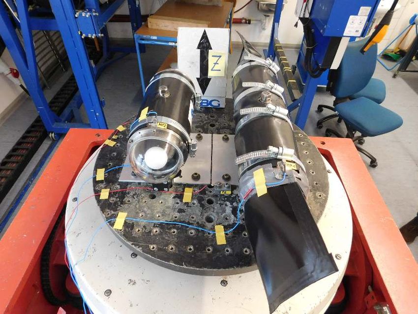
The instrument platform consists of a steel frame with plastic grid walls to which various
objects can be fastened. In the middle of the instrument platform a titanium junction box
is fastened, which acts as a distributor between node and instruments (Fig. 2.2). Smaller
[ONC1] Ocean Networks Canada Homepage. http://www.oceannetworks.ca/. accessed: 28.10.2018
[ONC2] Ocean Networks Canada Strategic Plan 2016-2021. http://www.oceannetworks.ca/sites/default/
files/pdf/ONCStrategicPlan2016-2021.pdf. accessed: 28.10.2018
[WT87] P. P. E. Weaver and J. Thomson. Geology and Geochemistry of Abyssal Plains. London: Geological
Society, 1987. isbn: 978-0-632-01744-7
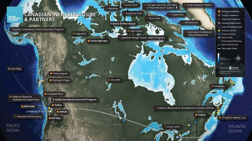
15Chapter 2. Ocean Networks Canada
Figure 2.1: Map of the observatories and stations of Ocean Networks Canada. The STRAW
strings are located in the Pacific Ocean, at the location marked for a future neutrino
observatory. Image courtesy of Ocean Networks Canada.
instruments can be fastened to the platform and are positioned after deployment by a
remotely controlled underwater vehicle (ROV). On two sides of the instrument platform
the Teledyne ODI plugs are located. Cables with the corresponding counterpart can be
connected to these underwater, as the plug releases a small amount of oil during plugging,
thus isolating the connection. The long cables connecting the instruments to the platform,
either Kevlar-enforced cables or cables in oil-filled hoses, hang in figure-eight loops on
horns at the sides of the platform. This allows the ROV to grab a cable end and fly into
position, the cable will unwind from the horns without contortion. The maximum cable
length is 70 m after which the transmission quality drops significantly.
In some cases instruments do not connect directly to the junction box. In this case
an additional intermediary, the mini junction box, is used. The mini junction box is a
development by ONC, hosting power converters, Ethernet switches, and microcontrollers
for monitoring and controlling the power supply to the instruments. Additionally, the mini
junction box contains a fault protection by checking all power lines against a seawater
reference. For STRAW, two mini junction boxes were used, one for each string, each
equipped with an additional circuit board developed at TUM for timing synchronisation
between the instruments.
ONC tests all instruments extensively before deployment. Apart from ensuring that the
instruments integrate into the network, several long term underwater tests are done with
the main focus on possible leakage and electric faults.
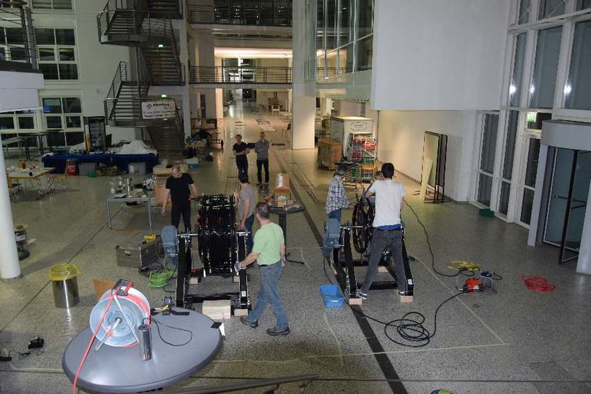
16Chapter 2. Ocean Networks Canada
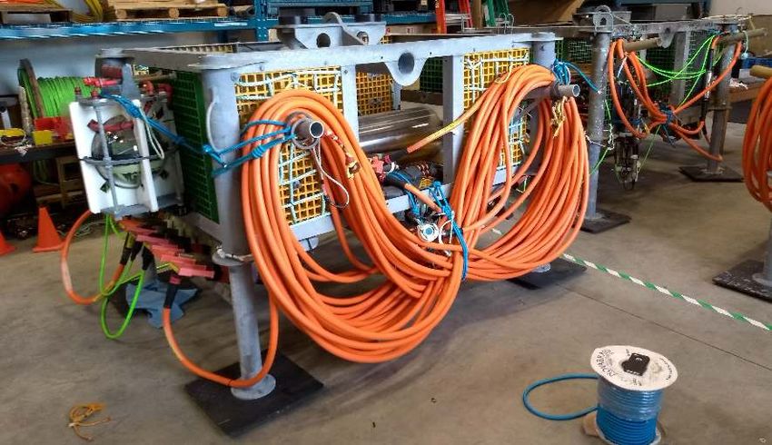
Figure 2.2: Instrument platforms at ONC. In the middle of the steel frame the titanium
junction box contains the electronics. On horns on the side an oil-filled hose with data
and power cables inside is laid in figure-eight loops. The ODI connectors for the cables
(bottom left) are equipped with large handles for ROV interaction. Lighter instruments
can be directly attached to the junction box (left: Titan accelerometer). When connecting
an instrument the ROV first removes the blue elastic straps holding the orange hose by
pulling out the securing pins. It then grabs the free end of the hose and flies to the target
instrument. Due to the figure-eight loops the hose unwinds from the junction box without
contortion.
2.3 Deployment method
For the deployment of instruments, ONC is supported by the Canadian Coast Guard.
Using a Coast Guard vessel, instruments are transported to the site. After necessary
inspections and maintenance of already existing instrumentation, instrument platforms
and instruments are deployed using the heavy lift line of the ship. Final steps for the
instrument setup are done on the back deck by ONC personnel. After deployment, a ROV
is lowered into the water, inspects the instruments, and makes the necessary connections
between instruments, junction box, and node. For the deployment of STRAW, the CCGS
John P. Tully served as deployment vessel. The deployment was streamed live and a
connection was kept to TUM.
2.4 Remotely Operated Platform for Ocean Science (ROPOS)
The ROPOS ROV (Fig. 2.4) by the Canadian Scientific Submersible Factory did the
underwater operations during the Tully cruise. Controlled by its own team of operators it
is lowered into the water on an umbilical and then navigated using its thrusters. Equipped
17Chapter 2. Ocean Networks Canada
Figure 2.3: One of the arms of the ROV. With trained operators the ROV is capable of
using these arms almost like human arms, holding tools for performing tasks such as
cutting rope or collecting samples.
with two mechanical arms and various cameras, it can perform various tasks including
collecting samples, using tools like cutters and position instruments. Via the umbilical of
the ship it has a thru-frame lift capacity of almost two tons; the arms themselves however
can not lift weights over 100 kg (Fig. 2.3).
18Chapter 2. Ocean Networks Canada
Figure 2.4: ROPOS from the back and the front while in an ONC workshop. On the back
side the two main thrusters and part of the buoyancy (yellow) are visible. From the front
we see the two arms (one covered by the ladder). Between the arms is a tray on which
during missions a box for tools and samples is placed. Various cameras and spotlights
guarantee good visual overview during mission.
19Chapter 3
Simulations and expected
environment
Before the planning of our strings, it was vital to estimate the environment, namely
the scattering and absorption length would influence our detector geometry, and the
background rate, as we would have to tailor our readout electronics to it.
3.1 Water transmittivity
The intensity I(x) of a narrow light cone in water can be described by using an exponen-
tial absorption law with l att the attenuation length, l abs the absorption length, and l scat
the scattering length:
I0 x I0 1 1
I(x) = exp − = exp −x + (3.1)
4πx2 l att 4πx2 l abs l scat
We distinguish between the scattering length l scat and the effective scattering length
l scat,eff . The scattering length describes the length after which a photon has been scattered
with a probability of 1 − 1/e. The effective scattering length takes into account the average
scattering angle. Especially when Mie scattering on large particles is dominant, the
angular distribution has a strong forward preference. The scattered photon therefore
often has only a minimal direction change [ANT05]. The effective scattering length
corrects for this with the average cosine of the scattering angle θ:
l scat
l scat,eff = − (3.2)
ln hcos θi
Whereas the scattering length is used for measurements with a narrow beam, as every-
thing scattered by only a few degrees is lost to the beam, the effective scattering length is
the relevant parameter when measurements with an isotropic light source are made.
In general, all of these lengths depend on the wavelength. Water, regardless of the site,
has a clear transmission window in the visible spectrum with its peak in the blue-green.
The relative transmission of wavelengths to each other is mostly constant, however, the
absolute values change heavily. This observation by Bradner [DUM] and Jerlov [Jer76] is
[ANT05] ANTARES Collaboration. “Transmission of light in deep sea water at the site of the Antares neutrino
telescope”. In: Astropart.Phys 23 (2005), pp. 131–155. doi: 10.1016/j.astropartphys.2004.11.006
[DUM] H. Bradner for the DUMAND Collaboration. Attenuation of light in clear deep ocean water. http:
//www.inp.demokritos.gr/web2/nestor/www/2nd/files/247_252_bradner.pdf
[Jer76] N.G. Jerlov. Marine Optics. Amsterdam: Elsevier, 1976. isbn: 978-0-080-87050-2
20Chapter 3. Simulations and expected environment
only true for deep sea waters, in coastal waters the relative transmissions can vary.
[Cap+02] have measured the transmission of several sites off the Italian coast in the
Mediterranean using an WetLabs AC9 transmissometer and have found attenuation
lengths of 50 m for blue light (412 nm) with a strong tendency for clearer water with
greater depth.
Measurements done by the ANTARES collaboration [ANT05] show comparable values.
Smith and Baker [SB81] have done measurements of pure sea water, cleaned from dust
particles, and made an extensive comparison of the measured values of other experiments.
They also agree on a maximum attenuation length of 50 m in the best case.
To the knowledge of the author, measurements of the deep Pacific water close to Cascadia
Basin have not been conducted so far, extensive measurements of surface water have been
done by Jerlov [Jer76]. Jerlov has characterized water into five coastal types and five
ocean types. His characterization of the Mediterranean surface water (Type IA) is in
good agreement with the previously mentioned measurements; the Canadian pacific coast
(Type III) has a four times shorter attenuation length, but this result must not necessarily
extend to the water at 2.5 km depth.
Based on these results, we assume an attenuation length between 15 m and 50 m. The
modules on our strings are therefore spaced at about 20 m with a string distance of 40 m
and an effective string length of 110 m. With this setup the distances between the modules
extend over few attenuation lengths in any expectable case.
In Fig. 3.1 we plotted the number of photons we expect to see in an SDOM for a POCAM
flash with 109 emitted photons. The data is based on an absorption spectrum taken from
[SB81]. While the absolute values may change depending on the absorption length at the
site, the overall picture gives us a good estimate of the dominant wavelengths.
3.2 The string in the current
A simulation was written in which the string with a buoyancy at the top is subjected
to the expected current of 0.1 ms−1 . At the time of the simulation, the final setup of the
string was not yet fixed, but adequate estimates of the relevant parameters, weight and
effective area, could already be made. Fig. 3.2 shows the results of the simulation. For
a buoyancy of 300 kg the string is displaced at the top by 4 m, whereas for 600 kg this
drops to 1.2 m. A large displacement would alter the distances between the modules
significantly, thus distorting the absorption length measurement. Allowing a small buffer
in case parts of the string should become heavier than expected, a buoyancy of 500 kg was
deemed to be a good value for an acceptable string tilt.
3.3 Preliminary light simulation
In order to obtain information about feasible detector geometries, the light propagation
in water was simulated. This simulation allowed us to estimate the effect of shadows,
caused e.g. by module mountings, the absolute intensity, and the ratio between scattered
and direct POCAM light received by a SDOM detector.
[Cap+02] A. Capone et al. “Measurements of light transmission in deep Sea with the AC9 transmissometer”.
In: Nucl.Instrum.Meth. A487 (2002), pp. 423–434. doi: 10.1016/S0168-9002(01)02194-5
[SB81] R. C. Smith and K. S. Baker. “Optical properties of the clearest natural waters”. In: Applied Optics 20
(2 1981), pp. 177–184
21Chapter 3. Simulations and expected environment
Number of detected photons
10m
104 30m
50m
70m
102
100
300 350 400 450 500 550 600 650 700
Wavelength [nm]
Figure 3.1: By using data from [SB81] we can estimate the light measured by a SDOM
when a POCAM pulse creates 109 photons. The efficiency of the photomultiplier of the
SDOM is already factored in. We see that for long ranges significant amounts of light can
only be detected in a small window from 450 − 550 nm.
The code written for this simulation uses Mie scattering. Rayleigh scattering, being
only a special case of Mie scattering with very small particles (molecules) is not treated
separately. Mie scattering describes the scattering of light in a medium, in which many
small spherical particles of a different refraction index are suspended [Mie08].
Because it is highly difficult to write numerically stable code describing Mie-scattering,
the BHMIE code by Bohren and Huffman [BH98] was used. The Fortran code by Bohren
and Huffman providing the scattering profile was compiled and linked to a propagation
simulation written in C++.
In general, the scattering of light in water is not the scattering on one type of particle, but
the scattering on many particles of different sizes, such as the water molecules themselves
(Rayleigh scattering) and various dust particles. For later data analysis the simulation can
easily be extended to this functionality; for the preliminary simulation, we only simulated
one type of particle at a time.
An early simulation simulated one POCAM and one SDOM at a set distance and orienta-
tion to each other. Due to the many possible orientations and distances this approach has
turned out to have little explanatory power and high computing power consumption.
To get a better overview over the parameter space the simulation was therefore changed
as follows: We no longer simulated two modules, instead only one POCAM is simulated.
The SDOM response could then be calculated looking at the angular distribution of the
POCAM light at a given distance and factoring in the effective area of the SDOM at a given
orientation. The disadvantage of this method is the neglect of the angular dependence
of the SDOM photomultipliers. For later data analysis this has to be factored in again,
for the preliminary simulation the results are nonetheless sufficient to rule out or favor
[Mie08] Gustav Mie. “Beiträge zur Optik trüber Medien, speziell kolloidaler Metallösungen”. In: Annalen
der Physik 330.3 (1908), pp. 377–445. doi: 10.1002/andp.19083300302
[BH98] Craig F. Bohren and Donald R. Huffman. Absorption and scattering of light by small particles. 2nd ed.
Wiley, 1998. isbn: 978-0-471-29340-8
22Chapter 3. Simulations and expected environment
300kg
400kg
100 500kg
Height [m]
600kg
50
0
0 0.5 1 1.5 2 2.5 3 3.5 4
Displacement [m]
Figure 3.2: Horizontal displacement of the string depending on the buoyancy. At the time
of the simulation the final setup of the string was not yet fixed, but adequate estimates
for weight and effective area were already available. The simulation assumes a current of
0.1 ms−1 .
certain detector geometries.
Fig. 3.3 and Fig. 3.4 show exemplary simulations for λ abs = 50 m, λ scat = 100 m and
very small particles (Rayleigh scattering). Many simulations have been done, varying the
parameters within the values that could be expected at Cascadia Basin. We do not show
the individual results here, as they all more or less match the results shown in Fig. 3.3
and Fig. 3.4 . The following conclusions can be drawn for all reasonable parameter sets.
First, the separation between scattered and unscattered light, and thus the calculation of
the scattering length, can be extremely difficult. Using a detector placed below a POCAM
flashing only its upper hemisphere could be helpful, as all light detected here is scattered.
We can compare this intensity to the measured intensity of a detector placed at the same
distance above the POCAM, directly looking at the flashing hemisphere, and thus separate
absorption and scattering. For the detector this can be realised either by two SDOMs at
the same distance, but above and below a POCAM, or by one POCAM and one SDOM,
when the POCAM flashes its hemispheres separately.
The second conclusion from the plots is that shadows cast by parts of the module
mounting or the strings themselves pose a big problem, as they are neither smeared out to
negligibility by scattering, nor sharp enough, so that they could be easily factored out of
the measured data by analytical means. This poses large restrictions on the mechanical
design of our string. Obviously the module mounting should cast as small a shadow
as possible. Additionally, the strings can not be allowed to twist, as this would mean
that steel rope and data cables would cast shadows between the modules. As a simple
example modules mounted to the side of two single steel wires strings can be considered.
With the water current all modules would rotate to the same side, as for example wind
vanes do. If the current were constant, we could place both strings perpendicular to the
current direction and the modules would have a clear line of sight to each other. However,
when the current direction is parallel to the line connecting the strings, meaning that one
23Chapter 3. Simulations and expected environment
Intensity [a.u.] ·104 ·104
Intensity [a.u.]
1.5
1
1
0.5 0.5
0 0
0 100 200 300 0 50 100 150
φ [deg] θ [deg]
Figure 3.3: A simulation of the POCAM in water with Rayleigh scattering, λ abs = 50 m,
λ scat = 100 m The light output was observed at 50 m distance. Left: both hemispheres are
flashing, the light distribution in φ was plotted. The POCAM was held between two steel
wires casting shadows. We see that the shadows are blurred and the blur extends over
about 60◦ . Right: light distribution in θ for a POCAM flashing only one hemisphere.
·104
1 600
Intensity [a.u.]
Intensity [a.u.]
0.8
0.6 400
0.4 200
0.2
0 0
0 0.5 1 1.5 0 0.5 1 1.5
t [µs] t [µs]
Figure 3.4: Simulation with the same parameters as in Fig. 3.3 . Only the upper hemi-
sphere is flashing. Left: time distribution of the light at 50 m distance for θ < 20◦ . We see
a sharp peak of direct light with a comparatively small tail of scattered light. Right: time
distribution for θ > 160◦ . Below the POCAM we see only scattered light. Both histograms
use the same scale on the y-axis.
string is behind the other, with all modules flowing behind their strings, the line of sight
is clearly blocked by one of the strings. Data provided by ONC shows that the current
at Cascadia Basin changes over the year and has no preferred direction. Thus, strings
resistant to rotation had to be developed.
24Chapter 4
The double string
As the previous chapter about preliminary light simulations showed, the strings need
some stability against twisting. It was unfeasible to make the strings out of a single steel
line that would by itself be stiff enough to resist twisting caused by the water current. This
single line would be extremely heavy and too stiff to be handled conveniently on the ship.
Instead many steel lines can be used to build a string. In the easiest configuration two
steel lines run parallel and are connected by spacers, which are stiff steel bars keeping the
lines apart at a fixed distance. The STRAW strings follow this design, two steel lines run
at 0.4m distance. Every 5 m a steel spacer clamps to both lines and keeps them at 0.4 m
distance. This concept can be compared to a rope ladder.
With such a design the resistance against twisting is provided by the fact that twisting
will shorten the double line, thus a strong buoyancy at the top, pulling on the string,
results in a certain string stiffness. It could be argued that the stiffness of steel ropes
themselves adds additional stiffness to the double line. However, it is very difficult to lay
out a long steel rope without any twists. Thus it becomes equally impossible to assemble
a string that has not a predisposition to twist in some direction, especially as one has to
consider that a twist-free steel rope might want to twist once tension is applied. Thus
the approach is to use steel ropes that have as little as possible stiffness themselves and
provide all of the string stiffness by a large buoy at the top. The stiffness of a double string
can be adjusted by the distance between the parallel wire ropes and the distance between
the spacers. Precise calculations are presented in Chapter 7.
Of course the stiffness could be improved by adding more lines to a string. A triple
string was considered, based on three steel ropes kept apart by triangular spacers. The
idea was discarded, as, unlike a single string or a double string, a triple string could not be
rolled up. Thus, storage, transportation, and deployment would have been significantly
more complicated.
On a double string the modules can either be positioned between the two steel ropes
or outside the steel ropes (Fig. 4.1). Positioning them in-between allows for a lighter
mounting. Positioning them outside requires a heavy mounting, adds the problem of tilt,
as the center of mass in no longer between the steel ropes, and provides bigger leverage
for the water current to twist the string, as the modules are the parts with the largest drag.
However, the big advantage of placing the modules outside is that the steel ropes and data
cables, whose shadows could disturb the measurements, are now on only one side of the
module. Thus the string could theoretically twist up to a value slightly below 180◦ before
the shadows would pose a problem. With the module between the steel ropes shadows
become a problem if the twist reaches a value close to 90◦ .
25Chapter 4. The double string
Figure 4.1: Possible string configurations. Left: a single wire rope, allowing the module to
rotate freely in the current. The stiffness of the wire rope can be neglected on a length of
up to 110 m. Middle: a module mounted between two wire ropes. Rotation is no longer
possible. Right: a module mounted to the side of two wire ropes. Rotation is not possible
and only one shadow is cast, as wire ropes lie in the same line of sight.
Figure 4.2: Double string and module mounting of STRAW at Cascadia Basin. Image
taken by the ROV after deployment.
At the same time as the string structure was developed we also considered the deploy-
ment mechanism. The concept of the winch, which is extensively described in Chapter
9, was developed. On a winch having the modules between the steel ropes means that
successive layer spooled onto the winch cover the modules, thus accessing them after the
string has been spooled becomes extremely difficult. If the modules are placed outside of
the steel ropes they would still be accessible on the winch.
Considering the last two arguments it was decided that the modules would be best
placed outside of the steel ropes (Fig. 4.2).
26Chapter 5
Modules
5.1 POCAM
The Precision Optical Calibration Module (POCAM) is an isotropic light source devel-
oped as a calibration device for IceCube Gen2 [Jur+16]. A previous version has already
been successfully tested in the Gigaton Volume Detector in Lake Baikal [Spa17]. At its
center are two semi-transparent PTFE (teflon) integrating spheres, which diffuse the light
of fast pulsed LEDs.
5.1.1 Housing
Designed to withstand the freezing pressure at the South Pole, the housing consists of a
titanium cylinder with two BK-7 glass hemispheres at a total length of 40 cm and a rating
of 1500 bar. In each hemisphere one integrating sphere illuminates 2π. At large distances
the light output of both hemispheres merges to an almost isotropic 4π illumination. The
glass hemispheres are glued to titanium flanges which are bolted to the main cylinder. A
vacuum plug for evacuation and an electrical plug penetrate the cylinder at opposite sites
(Fig. 5.3).
5.1.2 Integrating sphere
The integrating sphere was manufactured at TUM based on Geant4 simulations [Gär16]
and measurements [Hen18]. Using the special property of teflon to have a diffuse cosine
reflection (Lambertian reflection) as well as a diffuse cosine transmission at low thick-
nesses, a teflon sphere can completely diffuse the light of a light source with an arbitrary
emission profile (Fig. 5.4). The teflon sphere in the POCAM has a diameter of 50 mm and
a thickness of 1 mm and is placed above an array of six LEDs. Directly above the LEDs the
[Jur+16] M. Jurkovič et al. “A Precision Optical Calibration Module (POCAM) for IceCube-Gen2”. In: EPJ
Web Conf. 116 (2016), p. 06001. doi: 10.1051/epjconf/201611606001
[Spa17] Christian Spannfellner. Realisierung des ersten Precision Optical Calibration Modules für das Gigaton
Volume Detector Neutrino Teleskop in Baikal. BA thesis, https://www.cosmic- particles.ph.tum.de/
fileadmin/w00bkl/www/Thesis/BA_Christian_Spannfellner.pdf. July 2017
[Gär16] Andreas Gärtner. Realization of the “Precision Optical Calibration Module” prototype for calibration of
IceCube-Gen2. BA thesis, https://www.cosmic-particles.ph.tum.de/fileadmin/w00bkl/www/Thesis/
gaertner_BA.pdf. July 2016
[Hen18] Felix Henningsen. “Optical Characterization of the Deep Pacific Ocean: Development of an Optical
Sensor Array for a Future Neutrino Telescope”. MA thesis. Technical University of Munich, July 2018
27Chapter 5. Modules
Digital Board Analog Board
T T
I2C
H/T/p DC/DC SiPM
DC/DC PD
DATA
CLK ADC
Kapustinski TRG
SPI config
RS485
RS232 FPGA
µC
SPI user
µSD SPI
FRAM SPI Local CLK
External CLK
Loopback TRG
RTC External TRG
Figure 5.1: Scheme of the electronics of one POCAM hemisphere developed by M. Böhmer
of ZTL. A microcontroller handles communication and data storage, a FPGA deals with
sensor readout and LED triggering. Apart from the silicon photomultiplier (SiPM) and
the photo diode (PD) several environment sensors were used for temperature (T), pressure
(p), and humidity (H). A trigger signal from one FPGA travels to the other FPGA (External
TRG) and through a cable of the same length back to the original FPGA (Loopback TRG),
thus allowing synchronized triggering.
thickness of the sphere is only 0.5 mm in order to increase light yield. A detailed study on
the emission profile has been done in [Hen18].
5.1.3 In-situ calibration
Per hemisphere the POCAM has two sensors, a photo diode and a silicon photomultiplier,
monitoring the light output. This allows us to compensate to some extent effects such as
temperature changes and aging of components. Before readout, the signals are amplified
using a Cremat charge amplifier.
5.1.4 Electronics
The electronics of the POCAM were developed by Michael Böhmer of ZTL. Inside the
POCAM circuit boards are stacked on each flange (Fig. 5.2). The two hemispheres of the
28Chapter 5. Modules
Figure 5.2: Left: stacked circuit boards of a POCAM hemisphere. From top to bottom:
power board, digital board, analog board. Right: closeup view of one hemisphere on a
closed POCAM. Below the integrating sphere a piece of aluminium coated in a black low
gloss color with openings for the sensors. [Hen]
POCAM can operate independent of each other ensuring maximum redundancy. The
data connection to the outside is RS-485, the same protocol that was used for the Gigaton
Volume Detector. It is therefore the only module that can be more than 70 m away from a
mini junction box, which is the limiting distance for Ethernet communication through
the sub-sea cables. The RS-485 signal goes to each of the digital boards, one per flange,
holding a microcontroller for communication, data storage and slow control, as well as
a FPGA for sensor readout and LED triggering. The LEDs are driven by a Kapustinsky
circuit. Both microcontroller and FPGA can be updated remotely if necessary. The digital
board is stacked onto the analog board holding LEDs, Kapustinsky circuits, sensors, and
amplifiers. One central power board creates the necessary voltage for the microcontrollers
and houses the central clock. The FPGAs of both hemispheres have a direct connection,
allowing, after one has been set up as master and one as slave, a synchronized light pulse
from both hemispheres (Fig. 5.1).
5.1.5 Kapustinsky circuit
The LED driver, providing pulses of 109 photons at pulse lengths of below 10 ns, is
based on the design of Kapustinsky [Kap+85] with the modification proposed by [LV06].
The Kapustinsky flasher is based on a quick discharge of a capacitor through a LED, with
an inductance parallel to the LED shortening the pulse.
F. Henningsen of the STRAW team has done an extensive experimental characterization
of the impact of the inductance, the capacity and the voltage on the circuit as well as a
test of various LEDs, which have a significant impact on the pulse length. [Hen18]
[Kap+85] J.S. Kapustinsky et al. “A fast timing light pulser for scintillation detectors”. In: Nuclear Instruments
and Methods in Physics Research Section A: Accelerators, Spectrometers, Detectors and Associated Equipment
241.2 (1985), pp. 612–613. issn: 0168-9002. doi: 10.1016/0168- 9002(85)90622- 9. url: http://www.
sciencedirect.com/science/article/pii/0168900285906229
[LV06] B. K. Lubsandorzhiev and Y. E. Vyatchin. “Studies of ’Kapustinsky’s’ light pulser timing characteris-
tics”. In: JINST 1,T06001 (2006)
[Hen18] Felix Henningsen. “Optical Characterization of the Deep Pacific Ocean: Development of an Optical
Sensor Array for a Future Neutrino Telescope”. MA thesis. Technical University of Munich, July 2018
29You can also read