Race to the Bottom: Competition and Quality in Science
←
→
Page content transcription
If your browser does not render page correctly, please read the page content below
Race to the Bottom:
                         Competition and Quality in Science∗
                                    Ryan Hill†             Carolyn Stein‡

                                             November 5, 2020

                                                   Abstract

          This paper investigates how competition to publish first and thereby establish priority im-
      pacts the quality of scientific research. We begin by developing a model where scientists decide
      whether and how long to work on a given project. When deciding how long to let their projects
      mature, scientists trade off the marginal benefit of higher quality research against the marginal
      risk of being preempted. The most important (highest potential) projects are the most com-
      petitive because they induce the most entry. Therefore, the model predicts these projects are
      also the most rushed and lowest quality. We test the predictions of this model in the field of
      structural biology using data from the Protein Data Bank (PDB), a repository for structures of
      large macromolecules. An important feature of the PDB is that it assigns objective measures
      of scientific quality to each structure. As suggested by the model, we find that structures with
      higher ex-ante potential generate more competition, are completed faster, and are lower qual-
      ity. Consistent with the model, and with a causal interpretation of our empirical results, these
      relationships are mitigated when we focus on structures deposited by scientists who – by nature
      of their employment position – are less focused on publication and priority.

             This paper is updated frequently. The latest version can be found here.

  ∗
      We are immensely grateful to our advisors Heidi Williams, Amy Finkelstein, and Pierre Azoulay for their en-
thusiasm and guidance. Stephen Burley, Scott Strobel, Aled Edwards, and Steven Cohen provided valuable insight
into the field of structural biology, the Protein Data Bank, and the Structural Genomics Consortium. We thank
David Autor, Jonathan Cohen, Peter Cohen, Glenn Ellison, Chishio Furukawa, Colin Gray, Sam Hanson, Ariella
Kahn-Lang, Layne Kirshon, Matt Notowidigdo, Tamar Oostrom, Jonathan Roth, Adrienne Sabety, Michael Stepner,
Alison Stein, Jeremy Stein, Sean Wang, Michael Wong, and participants in the MIT Labor and Public Finance lunches
for their thoughtful comments and discussions. This material is based upon work supported by the National Science
Foundation Graduate Research Fellowship under Grant No. 1122374 (Hill and Stein) and the National Institute of
Aging under Grant No. T32-AG000186 (Stein). All remaining errors are our own.
    †
      Northwestern University, Kellogg School of Management, ryan.hill@kellogg.northwestern.edu.
    ‡
      MIT Economics Department, cstein@mit.edu. Job Market Paper.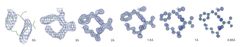
1    Introduction
Credit for new ideas is the primary currency of scientific careers. Credit allows scientists to build
reputations, which translate to grant funding, promotion, and prizes (Tuckman and Leahey, 1975;
Diamond, 1986; Stephan, 1996). As described by Merton (1957), credit comes — at least in part
— from disclosing one’s findings first, thereby establishing priority. It is not surprising, then, that
scientists compete intensely to publish important findings first. Indeed, scientific history has been
punctuated with cutthroat races and fierce disputes over priority (Merton, 1961; Bikard, 2020).1
This competition and fear of pre-emption or “getting scooped” is not uniquely felt by famous sci-
entists, but rather permeates the field. Older survey evidence from Hagstrom (1974) suggests that
nearly two thirds of scientists have been scooped at least once in their careers, and a third of sci-
entists reported being moderately to very concerned about being scooped in their current work.
Newer survey evidence focusing on experimental biologists (Hong and Walsh, 2009) and structural
biologists more specifically (Hill and Stein, 2020) suggests that pre-emption remains common, and
that the threat of pre-emption continues to be perceived as a serious concern.
    Competition for priority has potential benefits and costs for science. Pressure to establish prior-
ity can hasten the pace of discovery and incentivize timely disclosure (Dasgupta and David, 1994).
However, competition may also have a dark side. For years, scientists have voiced concerns that
the pressure to publish quickly and preempt competitors may lead to “quick and dirty experiments”
rather than “careful, methodical work” (Yong, 2018; Anderson et al., 2007). As early as the nine-
teenth century, Darwin lamented the norm of naming a species after its first discoverer, since this put
“a premium on hasty and careless work” and rewarded “species-mongers” for “miserably describ[ing]
a species in two or three words” (Darwin, 1887; Merton, 1957). More recently, journal editors have
bemoaned what they view as increased sloppiness in science: “missing references; incorrect controls;
undeclared cosmetic adjustments to figures; duplications; reserve figures and dummy text included;
inaccurate and incomplete methods; and improper use of statistics” (Nature Editors, 2012). In
other words, the faster pace of science has a cost: lower quality science. The goal of this paper is to
consider the impact of competition on the quality of scientific work. We use data from the field of
structural biology to empirically document that more competitive projects are executed with poorer
quality. A variety of evidence supports a causal interpretation of competition leading researchers
to rush to publication, as opposed to other omitted factors.
    Economists have long studied innovation races, often in the context of patent or commercial R&D
races. There is a large theoretical literature which considers the strategic interaction between two
teams racing to innovate. These models have varied and often contradictory conclusions, depending
on how the innovative process is modeled. For example, in models where innovation is characterized
   1
     To name but a few examples: Isaac Newton and Gottfried Leibniz famously sparred over who should get credit
as the inventor of calculus. Charles Darwin was distraught upon receiving a manuscript from Alfred Wallace, which
bore an uncanny resemblance to Darwin’s (yet unpublished) On the Origin of Species (Darwin, 1887). More recently,
Robert Gallo and Luc Montagnier fought bitterly and publicly over who first discovered the HIV virus. The dispute
was so acrimonious (and the research topic so important) that two national governments had to step in to broker a
peace (Altman, 1987).

                                                       1
as a single, stochastic step, scientists will compete vigorously (Loury, 1979; Lee and Wilde, 1980). By
contrast, if innovation is a step-by-step process, where experience matters and progress is observable,
then the strategic behavior may be more nuanced (Fudenberg et al., 1983; Harris and Vickers, 1985,
1987; Aghion et al., 2001).2 However, a common feature of these models is that innovation is binary:
the team either succeeds or fails to invent. There is no notion that the invention may vary in its
quality, depending on how much time or effort was spent. There are a few exceptions to this rule:
Hopenhayn and Squintani (2016) and Bobtcheff et al. (2017) explicitly model the tension between
letting a project mature longer (thereby improving its quality) versus patenting or publishing quickly
(reducing the probability of being preempted). Tiokhin et al. (2020) develop a model of a similar
spirit, where researchers choose a specific dimension of quality — the sample size. Studies with
larger sample sizes take longer to complete, and so more competition leads to smaller sample sizes
and less reliable science. Tiokhin and Derex (2019) test this line of thinking in a lab experiment.
       Along these same lines, we develop a model of how competition spurred by priority races impacts
the quality of scientific research. In our model, there is a deterministic relationship between the time
a scientist spends on a project and the project’s ultimate scientific quality. The scientist will choose
how long to work on a given project with this relationship in mind. However, multiple scientists may
be working on any given project. Therefore, there is always a latent threat of being pre-empted.
The scientist who finishes and publishes the project first receives more credit and acclaim than the
scientist who finishes second. This implies that a scientist deciding how long to work on her project
must trade off the returns to continued “polishing” against the threat of potentially being scooped.
As a result, the threat of competition leads to lower quality projects than if the scientist know she
was working in isolation.
       However, in a departure from the other models cited above, we embed this framework in a model
where project entry is endogenous. This entry margin is important, because we allow for projects
to vary in their ex-ante potential. To understand what we mean by “potential,” consider that some
projects solve long-standing open questions or have important applications for subsequent research.
A scientist who completes one of these projects can expect professional acclaim, and these are the
projects we consider “high-potential.” Scientists observe this ex-ante project potential, and use
this information to decide how much they are willing to invest in hopes of successfully starting the
project. This investment decision is how we operationalize endogenous project entry. High-potential
projects are more attractive, because they offer higher payoffs. As a result, researchers invest more
trying to enter these projects. Therefore, the high-potential projects are more competitive, which
in turn leads scientists to prematurely publish their findings. Thus, the key prediction of the model
is that high-potential projects — those tackling questions that the scientific community has deemed
the most important — are the projects that will also be executed with the lowest quality.
       While the model provides a helpful framework, the primary contribution of this paper is to
provide empirical support for the its claims. The idea that competition may lead to lower quality
   2
     This literature has been primarily theoretical, though there are a few exceptions. Cockburn and Henderson
(1994) study strategic behavior in drug development. Lerner (1997) studies strategic interaction between leaders and
followers in the disk drive industry.

                                                         2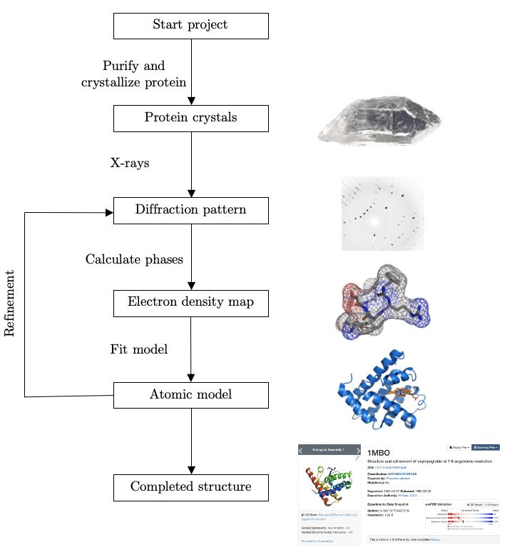
work is intuitive, and many scientists and journalists have speculated that this is the case (Fang
and Casadevall, 2015; Vale and Hyman, 2016; Yong, 2018). However, systematically measuring the
quality of scientific work is difficult. Consider the field of economics, for example — even with
significant expertise, it is difficult to imagine “scoring” papers based on their quality of execution in
a consistent, objective manner. Moreover, doing so at scale is infeasible.3
       We make progress on the challenge of measuring scientific quality in the field of structural biology
by using a unique data source called the Protein Data Bank (PDB). The PDB is a repository for
structural coordinates of biological macromolecules (primarily proteins). The data are contributed
by the worldwide research community, and then centralized and curated by the PDB. Importantly,
every macromolecular structure is scored on a variety of quality metrics. At a high level, structural
biologists are concerned with fitting three-dimensional structure models to experimental data, and
so these quality metrics are measures of goodness of fit. They allow us to compare quality across
different projects in an objective, science-based manner. To give an example of one of our quality
metrics, consider refinement resolution, which measures the distance between crystal lattice planes.
Nothing about this measure is subjective, nor can it be manipulated by the researcher.4 Figure
1 shows the same protein structure solved at different refinement resolutions, to illustrate what a
higher quality protein structure looks like.
       The rich data in the PDB also allow us to construct additional variables necessary to test our
model. The PDB groups identical proteins together into “similarity clusters” — proteins within
the same cluster are identical or near-identical. By counting the number of deposits in a similarity
cluster within a window of time after the first deposit, we can proxy for the competition researchers
solving that structure likely faced. If we see multiple deposits of the same structure uploaded to the
PDB in short succession, then researchers were likely engaged in a competitive race to deposit and
publish first. Moreover, the PDB includes detailed timelines for most structures. In particular, they
note the collection date (the date the researcher collected her experimental data) and the deposition
date (roughly the date the researcher finished her manuscript). The difference in these two dates
approximates the maturation period in the model.
       The PDB has no obvious analog to project importance or potential, which is a pivotal variable
in our model. Therefore, we use the rich meta-data in the PDB to construct our own measure.
Rather than use ex-post citations from the linked publications as our measure of ex-ante potential
(which might conflate potential with the ex-post quality of the work), we leverage the extensive
structure-level covariates in the PDB to instead predict citations. These covariates include detailed
characteristics of the protein known to the scientist before she begins working on the structure,
such as the protein type, the protein’s organism, the gene-protein linkage, and the prior number of
papers written about the protein. Because the number of covariates is large relative to the number
   3
      Some studies (Hengel, 2018) have used text analysis to measure a paper’s readability as a proxy for paper quality,
but such writing-based metrics fail to measure the underlying scientific content. Another strategy might be to use
citations, but this fails to disentangle the quality of the project from the importance of the topic or the prominence
of the author (Azoulay et al., 2013).
    4
      Though of course researchers can “target” certain quality measures, in an attempt to reach a certain threshold.

                                                           3
of observations, overfitting is a concern. To avoid this, we implement Least Absolute Shrinkage and
Selection Operator (LASSO) to select our covariates, and then impute the predicted values.
We use our computed values of potential to test the key predictions of the model. Comparing
structures in the 90th versus 10th percentile of the potential distribution, we find that high-potential
projects induce meaningfully more competition, with about 30 percent more deposits in their simi-
larity cluster. This suggests that researchers are behaving rationally by pursuing the most important
(and highest citation-generating) structures. We then look at how potential impacts maturation
and quality. We find that high-potential structures are completed about two months faster, and
have quality measures that are about 0.7 standard deviations lower than low-potential structures.
These results echo recent findings by a pair of structural biologists (Brown and Ramaswamy, 2007),
who show that structures published in top general interest journals tend to be of lower quality than
structures published in less prominent field journals.
However, a concern when interpreting these results is that competition and potential might be
correlated with omitted factors that are also correlated with quality. In particular, we are concerned
about complexity as an omitted variable — if competitive or high-potential structures are also more
difficult to solve, our results may be biased. We take several approaches to address this concern.
First, we investigate how long scientists spend working on their projects. If competitive and high-
potential projects are more complex, we would expect researchers to spend longer on these projects
in the absence of competition. However, we find the exact opposite: researchers spend less time on
more competitive and higher potential projects. This suggests that complexity alone cannot explain
our results, and that racing concerns must be at play. We also attempt to control for complexity
directly. This has a minimal effect on the magnitude of our estimates.
To further probe this concern, we leverage another source of variation – namely, whether the
protein was deposited by a structural genomics group. The majority of PDB structures are deposited
by university- or industry-based scientists, both of which face the types of incentives we have
described to publish early and obtain priority. In contrast, structural genomics (SG) researchers are
federally-funded scientists with a mission to deposit a variety of structures, with the goal of obtaining
better coverage of the protein-folding space and make future structure discovery easier. Qualitative
evidence suggests these groups are less focused on publication and priority, which is consistent with
the fact that only about 20 percent of SG structures ever appear in journal publications, compared
to over 80 percent of non-SG structures.
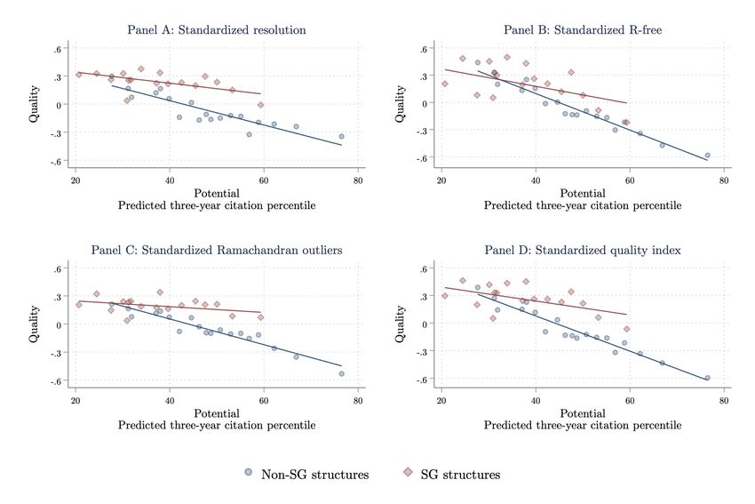
Because the SG groups are less motivated by competition, we can contrast the relationships
between potential and quality for SG structures versus non-SG structures. If complexity is correlated
with potential, then this should be the case for both the SG and non-SG structures. Intuitively,
by comparing the slopes across both groups, we thus “net out” the potential omitted variables
bias. Consistent with competition acting as the causal channel, we find more negative relationships
potential and quality among non-SG (i.e., more competitive) structures.
The fact that the most scientifically important structures are also the lowest quality intuitively
seems suboptimal from a social welfare perspective. If project potential and project quality are
4complements (as we assume in the model), then a lack of quality among high-potential projects
is particularly costly from a welfare perspective. Indeed, relative to a first-best scenario in which
a social planner could dictate both investment and maturation to each researcher, the negative
relationship between potential and quality does imply a welfare loss.
However, the monitoring and coordination costs make this type of scheme unrealistic from a
policy perspective. Instead, we consider a different policy lever: allowing the social planner to
dictate the division of credit between the first- and second-place teams. We consider this policy
response in part because some journals have recently enacted “scoop protection” policies5 explicitly
aimed at increasing the share of credit awarded to teams who lose priority races. We then ask:
with this single policy lever, can the social planner jointly achieve the optimal level of investment
and maturation? Our model suggests no. While making priority rewards more equal does increase
maturation periods toward the socially optimal level, it simultaneously may reduce investment
levels. If the social planner values the project more than the individual researcher (consistent with
the notion of research generating positive spillovers), then this reduced investment may be costly
from a social welfare perspective. The optimal choice of how to allocate credit depends on the
balance of these two forces, but ultimately may lead to a credit split that is lopsided. This in turn
will lead to the observed negative relationship between potential and quality. Therefore, while this
negative relationship tells us we are not at an unconstrained first-best, it cannot rule out that we
are at a constrained second-best.
The remainder of this paper proceeds as follows. Section 2 presents the model. Section 3
describes our setting and data. Section 4 tests the predictions of the model, and Section 5 considers
the welfare and policy implications. Section 6 concludes.
2 A Model of Competition and Quality in Scientific Research
The idea that competition for priority drives researchers to rush and cut corners in their work is
intuitive. Our goal in this section is to develop a model that formalizes this intuition, and that
generates additional testable predictions. Scientists in our model are rational agents, seeking to
maximize the total credit or recognition they receive for their work. This is consistent with views
put forth by Merton (1957) and Stephan (2012), though it stands in contrast with the idea that
scientists are purely motivated by the intrinsic satisfaction derived from “puzzle-solving” (Hagstrom,
1965).
The model has two stages. In the first stage, a scientist decides how much effort to invest in
starting the project. More investment at this stage translates to a higher probability of successfully
starting the project. We call this the entry decision. When making this decision, a scientist will
take into account each project’s potential payoffs, and weigh these against the costs of investing.
In the second stage, the scientist then decides how long to let the project mature. The choice of
5
These policies ask reviewers to treat recently scooped papers as if they are novel contributions; see Section 5.2.2
for more detail and examples.
5project maturation involves a tradeoff between higher project quality and an increasing probability
of getting scooped.
We begin by solving the second-stage problem. In equilibrium, the researcher will know the
probability that her competitor has entered the race, and she will have some prior on whether she
is ahead of or behind her competitor. She will use these pieces of information to trade off marginal
quality gains against the threat of pre-emption. The threat of competition will drive her to complete
her work more quickly than if there were no competition (or if she were naïve to this threat). This
provides us with our intuitive result that competition leads to lower scientific quality.
In the first stage, the researcher decides how much to invest in an effort to start the project,
taking second-stage decisions as given. Projects have heterogenous payoffs, with important projects
yielding more recognition than incremental projects. Scientists factor these payoffs into their in-
vestment decision. Therefore, the model generates predictions about which projects are the most
competitive (i.e., induce the most entry) and thus the lowest quality. Because the highest expected
payoff (i.e., the most important or “highest potential”) projects offer the largest rewards, it is exactly
these projects that our model predicts will have the most entry, competition, and rushing. This
leads to the key insight from our model: the most ex-ante important projects are executed with the
lowest quality ex-post. In the following sections, we formalize the intuition laid out above.
2.1 Preliminaries
Players. There are two symmetric scientists, i and j. Throughout, i will index an arbitrary
scientist and j will index her competitor. Both scientists are working on the same project and only
receive credit for their work once they have disclosed their findings through publication.
Timing, Investment, and Maturation. Time is continuous and indexed by t. From the per-
spective of each scientist, the model consists of two stages. In the first stage, scientist i has an
idea. We denote the moment the idea arrives as the start time, or tSi . However, the scientist must
pay an upfront cost in order to pursue the idea. At tSi , scientist i must decide how much to invest
in starting the project. If she invests Ii , she has probability g (Ii ) ∈ [0, 1] of successfully starting
the project, where g(·) is an increasing, concave function and the Inada conditions hold. These
assumptions reflect that more investment results in a higher probability of successfully entering a
project, but that the returns are diminishing. I could be resources spent writing a grant proposal or
trying to generate preliminary results. In our setting, a natural interpretation is that I represents
the time and resources spent trying to grow a protein crystal.6
The second stage occurs if the scientist successfully starts the project. Then, she must decide
how long to work on the project before publicly disclosing her findings. Let mi denote the time she
spends on the project, or the “maturation period.” The project is then complete at tFi = tSi + mi .
6
Indeed, the laborious process of growing protein crystals is almost universally a prerequisite for receiving a grant;
the NIH typically to takes a “no crystals, no grant” stance on funding projects in structural biology (Lattman, 1996).
6Payoffs and Credit Sharing. Projects vary in their ex-ante potential, which we denote P . For
example, an unsolved protein structure may be relevant for drug development, and therefore a
successful structure determination would be published in a top journal and be highly cited. We call
this a “high-potential” protein or project.
Projects also vary in their ex-post quality, depending on how well they are executed. Quality is a
deterministic function of the maturation period, which we denote Q(m). Q is an increasing, concave
function and the Inada conditions hold. Without loss of generality, we impose that limm→∞ Q(m) =
1. This facilitates the interpretation of quality as the share of the project’s total potential that the
researcher achieved. Then the total value of the project is the product of potential and quality.
The first team to finish a project receives a larger professional benefit (through publication,
recognition, and citations) than the second team. To operationalize this idea as generally as possible,
we say that the first team receives a reward equal to θ times the project’s value (through publication,
recognition, and citations). The second team receives a smaller benefit, equal to θ times the project’s
value. If r denotes the discount rate, then the present-discounted value of the project to the first-
place finisher is given by:
θe−rm P Q(m). (1)
Similarly, the present-discounted value of the project to the second-place finisher is given by:
θe−rm P Q(m). (2)
We make no restrictions on these weights, other than to specify that they are both positive and
θ ≥ θ. Importantly, we do not assume that the race is winner-take-all (i.e., θ = 0), as is common
in the theoretical patent and priority race literature (for example, Loury (1979); Fudenberg et al.
(1983); Bobtcheff et al. (2017)). Rather, consistent with empirical work on priority races (Hill and
Stein, 2020) and anecdotal evidence (Ramakrishnan, 2018), we allow for the second-place team to
share some of the credit.
Information Structure. The competing scientists have limited information about their competi-
tor’s progress in the race. Scientist i does not observe Ij , and so she doesn’t know the probability
her opponent enters, although she will have correct beliefs about this probability in equilibrium. In
addition, she does not know her competitor’s start time tSj . All she knows is that it is uniformly
distributed around her own start time. In other words, she believes that tSj ∼ Unif tSi − ∆, tSi + ∆
for some ∆ > 0. Figure 2 summarizes the model setup.
2.2 Maturation
We begin by solving the second stage problem of the optimal maturation delay, taking the first stage
investment as given. In other words, we explore what the scientist does once she has successfully
entered the project, and all her investment costs are already sunk. Our setup is similar to the
approach of Bobtcheff et al. (2017), but an important distinction is that we only allow the project’s
7value to depend on the maturation time m, and not on calendar time t. This simplifies the second
stage problem, and allows us to embed the solution into the first stage investment decision in a
more tractable way.
2.2.1 The No Competition Benchmark
We start by solving for the optimal maturation period of a scientist who knows that she is not
competing for priority. Alternatively, we could consider this the behavior of a naive scientist, who
does not recognize the risk of being scooped. This will serve as a useful benchmark once we re-
introduce the possibility of competition.
Without competition, the scientist simply trades off the marginal benefit of further maturation
∗
against the marginal cost of time discounting. The optimal maturation delay mN
i
C is given by
C∗
mN ∈ arg max e−rmi P Q (mi ) .
i (3)
mi
Taking the first-order condition and re-arranging (dropping the i subscripts for convenience) yields
∗
Q0 mN C
= r. (4)
Q (mN C ∗ )
In other words, the scientist will stop work on the project and publish the paper when the rate of
improvement equals the discount rate.
2.2.2 Adding Competition
We continue to study the problem of the scientist who has already entered the project and already
sunk the investment cost. However, now we allow for the possibility of a competitor. We call
∗
the solution to this problem the optimal maturation period with competition, and denote it mC
i .
∗
Scientist i believes that her competitor has also entered the project with some probability g(IjC ),
∗
where IjC is j’s equilibrium first-stage investment. However, because investment is sunk in the
∗
first stage, we can treat g(IjC ) as a parameter (simply g) in this part of the model to simplify the
notation.
While scientist i knows the probability that j entered the project, she does not know her potential
competitor’s start time, tSj . As described above, her prior is that tSj is uniformly distributed around
her own start time. Let π (mi , mj ) denote the probability that scientist i wins the race, conditional
on successfully entering. This can be written as
π(mi , mj ) = (1 − g) + gP r(tFi < tFj ) = (1 − g) + gP r(tSi + mi < tSj + mj ). (5)
The first term represents the probability that j fails to enter (and so i wins for sure), and the second
8term is the probability that j enters, but i finishes first. The optimal maturation period is given by
∗ −rm
mC
i ∈ arg max e P Q (mi ) π(mi , mj )θ + (1 − π(mi , mj )) θ . (6)
i
mi
The term outside the square brackets represents the full present discounted value of the project.
The terms inside the brackets denote i’s expected share of the credit, conditional on i successfully
starting the project. The product of these two terms is scientist i’s expected payoff conditional on
successfully starting the project. Taking the first-order condition of Equation 6 implicitly defines
scientist i’s best-response function, which depends on mj and other parameters:
∗
Q0 mC
i 1
C ∗ = r + . (7)
Q mi ∆ 2θ−g(θ−θ) + mj − mC∗
g(θ−θ) i
If we look for a symmetric equilibrium, this yields Proposition 1 below.
Proposition 1. Assume that first stage equilibrium investment is equal for both researchers, i.e.,
∗ ∗ ∗
IiC = IjC = I C . Further assume that ∆ is sufficiently large. Then in the second stage, there is a
∗ ∗ ∗ ∗
unique symmetric pure strategy Nash equilibrium where mC
i = mC
j = m
C and mC is implicitly
defined by
∗ ∗
Q0 mC g(I C )(θ − θ)
= r + . (8)
Q (mC ∗ ) ∆ 2θ − g(I C ∗ )(θ − θ)
Proof. See Appendix A.1.
Because Q(m) is increasing and concave, we know Q0 /Q is a decreasing function. Therefore, by
comparing Equations 4 and 8, we can see that mN C > mC . In other words, competition leads to
shorter maturation periods. This shortening is exacerbated when the difference between θ and θ is
large (priority rewards are more lopsided), ∆ is small (competitors start the projects close together,
and so the “flow risk” of getting scooped is high), or when g is close to one (the entry of a competitor
is likely). On the other hand, if θ = θ (first and second place share the rewards evenly), ∆ → ∞
(competition is very diffuse, so the “flow risk” of getting scooped is low), or g = 0 (the competitor
doesn’t enter), then we recover the no competition benchmark.
2.3 Investment
In the first stage, scientist i decides how much she would like to invest in hopes of starting the
project. Let Ii denote this investment, and let g (Ii ) be the probability she successfully enters the
project, where g is an increasing, concave function. With probability 1 − g (Ii ) she fails to enter the
project, and her payoff is zero. With probability g (Ii ) she successfully enters the project, and begins
work at tSi . Once she enters, there are two ways she can win the priority race: first, if her competitor
fails to enter, she wins for sure. Second, if her competitor enters but she finishes first, she also wins.
In either case, she gets a payoff of θP Q mC
i . On the other hand, if her competitor enters and she
9loses, her payoff is θP Q mC
i . Putting these pieces together (noting that in equilibrium, if both i
and j enter, they are equally likely to win) and re-arranging, the optimal level of investment is
∗ −rmC
∗ ∗ 1
IiC mC
∈ arg max g (Ii ) e i PQ i θ − g (Ij ) θ − θ − Ii . (9)
Ii 2
Taking the first-order condition of Equation 9 implicitly defines scientist i’s best-response function,
∗
which depends on Ij , mC
i , and other parameters:
∗ 1
g 0 (IiC ) = ∗ . (10)
−rmC C∗ θ − 12 g (Ij ) θ − θ
e i P Q mi
If we look for a symmetric equilibrium, this yields Proposition 2 below.
Proposition 2. Assume that researchers are playing a symmetric pure strategy Nash equilibrium
when selecting m in the second stage. Then, in the first stage, there is a unique symmetric pure
strategy Nash equilibrium where IiC = IjC = I C and IiC is implicitly defined by
∗ 1
g 0 (I C ) = . (11)
−rmC ∗ C∗ ) θ − 12 g (I C ∗ ) θ − θ
e P Q (m
Together with Proposition 1, this shows that there is a unique symmetric pure strategy Nash equilib-
rium for both investment and maturation.
Proof. See Appendix A.1.
Equations 11 and 8 together define the optimal investment level and maturation period for
scientists when entry into projects is endogenous. This allows us to prove three key results.
Proposition 3. Consider an exogenous increase in the probability of project entry, g. This corre-
sponds to an increase in competition, because it makes racing more likely. When projects become
more competitive, the maturation period becomes shorter and projects become lower quality. In other
∗ ∗
dmC dQ(mC )
words, dg < 0 and dg < 0.
Proof. See Appendix A.1. Scientist i selects mC
i by considering the probability that her competitor
enters g(Ij ). If this probability goes up, she will choose a shorter maturation period which results
in lower quality.
Proposition 4. Higher potential projects generate more investment and are therefore more com-
∗ ∗
dI C dg(I C )
petitive. In other words, dP > 0 and dP > 0.
Proof. See Appendix A.1. Scientist i will invest more to enter a high-potential project. Her com-
petitor will do the same. In equilibrium, high-potential projects are more likely to result in priority
races.
Proposition 5. Higher potential projects are completed more quickly, and are therefore of lower
∗ ∗
dmC dQ(mC )
quality. In other words, dP < 0 and dP < 0.
10Proof. This comes immediately from Propositions 3 and 4, by applying the chain rule.
3 Structural Biology and the Protein Data Bank
This section provides some scientific background on structural biology and describes our data. We
take particular care to explain how we map key variables from our model into measurable objects in
our data. Our empirical work focuses on structural biology precisely because there is such a clean
link between our theoretical model and our empirical setting. Section 3.1 provides an overview of the
field of structural biology, while sections 3.2 and 3.3 describe our datasets. Section 3.4 describes how
we construct our primary analysis sample and provides summary statistics. Appendix B provides
additional detail on our data sources and construction.
3.1 Structural Biology
Structural biology is the study of the three-dimensional structure of biological macromolecules,
including deoxyribonucleic acid (DNA), ribonucleic acids (RNA), and most commonly, proteins.
Understanding how macromolecules perform their functions inside of cells is one of the key themes
in molecular biology. Structural biologists shed light on these questions by determining the three-
dimensional arrangement of a protein’s atoms.
Proteins are composed of building blocks called amino acids. These amino acids are arranged
into a single chain, which folds up onto itself, creating a three-dimensional structure. While the
shape of these proteins is of great interest to researchers, the proteins themselves are too small
to observe directly under a microscope.7 Therefore, structural biologists use experimental data to
propose three-dimensional models of the protein shape to better understand biological function.
Structural biology has several unique features that make it amenable for our purposes (see
Section 3.1.1 below), but it is also an important field of science. Proteins contribute to nearly
every process inside the body, and understanding the shape and structure of proteins is critical to
understanding how they function. Moreover, many heritable diseases — such as sickle-cell anemia,
Alzheimer’s disease, and Huntington’s disease — are the direct result of protein mis-folding. Protein
structures also play a critical role in drug development and vaccine design (Westbrook and Burley,
2018). Protease inhibitors, a type of antiretroviral drug used to treat HIV, are one important
example of successful structure-based drug design (Wlodawer and Vondrasek, 1998). The rapid
discovery and deposition of the SARS-CoV-2 spike protein structure has proven to be a key input
in the ongoing development of COVID-19 vaccines and therapeutics (Wrapp et al., 2020). Over a
dozen Nobel prizes have been awarded for advances in the field (Martz et al., 2019).
7
Recent developments in the field of cryo-electron microscopy now allow scientists to observe larger structures
directly (Bai et al., 2015). However, despite the recent growth in this technique, fewer than five percent of PDB
structures deposited since 2015 have used this method.
113.1.1 Why Structural Biology?
Our empirical work focuses on the field of structural biology for several reasons. First, and most
importantly, structural biology has unique measures of objective project quality. Scientists in this
field work to solve the three-dimensional structure of known proteins, and there are several measures
of how precise and correct their solutions are. We will discuss these measures in the subsequent
sections, but we want to highlight the importance of this feature: it is difficult to imagine how one
might objectively rank the quality (distinct from the importance or relevance) of papers in other
fields, such as economics or mathematics. Our empirical work hinges on the fact that structural
biologists have developed unbiased, science-based measures of structure quality.
Second, we can measure competition and racing behavior using biological similarity measures
and project timelines. By comparing the amino acid sequences of different proteins, we can detect
when two proteins are similar or identical to one another. This allow us to find projects that focus
on similar proteins, while the timeline data allows us to determine if researchers were working on
these projects contemporaneously. Together, this allows us to determine which structures faced
heavy competition while the scientists were doing their research.
Third, the PDB contains rich descriptive data on each protein structure. For each structure, we
observe covariates like the detailed protein classification, the taxonomy / organism, and the associ-
ated gene. Together, these characteristics allow us to develop measures of the protein’s importance,
based purely on ex-ante characteristics — a topic we discuss in more detail in Section 4.1.
3.1.2 Solving Protein Structures Using X-Ray Crystallography
How do scientists solve protein structures? Understanding this process is important for interpreting
the various quality measures used in our analysis. We focus on proteins solved using a technique
called x-ray crystallography. The vast majority (89 percent) of structures are solved using this
method.
X-ray crystallography broadly consists of three steps (see Figure 3). Individual proteins are too
small to analyze or observe directly. Therefore, as a first step, the scientist must distill a concentrated
solution of the protein into orderly crystals. Growing these crystals is a slow and difficult process,
often described as “more art than science” (Rhodes, 2006) or at times simply “dumb luck” (Cudney,
1999). Success typically comes from trial and error, and a healthy dose of patience.8
Next, the scientist will bring her crystals to a synchrotron facility and subject the crystals to
x-ray beams. The crystal’s atom planes will diffract the x-rays, leading to a pattern of spots called
a “diffraction pattern.” Better (i.e., larger and more uniform) crystals yield superior diffraction
8
As Cudney colorfully explains: “How many times have you purposely designed a crystallization experiment and
had it work the first time? Liar. Like you really sit down and say ‘I am going to use pH 6 buffer because the p1 of
my protein is just above 6 and I will use isopropanol to manipulate the dielectric constant of the bulk solvent, and
add a little BOG to mask the hydrophoic interactions between sample molecules, and a little glycerol to help stabilize
the sample, and [a] pinch of trimethylamine hydrochloride to perturb water structure, and finally add some tartate
to stabilize the salt bridges in my sample.’ Right...Finding the best crystallization conditions is a lot like looking for
your car keys; they’re always the last place you look” (Cudney, 1999).
12patterns and improved resolution. If the scientist is willing to spend more time improving her
crystals — by repeatedly tweaking the temperature or pH conditions, for example — she may be
rewarded with better experimental data.
Finally, the scientist will use these diffraction patterns to first build an electron density map,
and then an initial atomic model. Building the atomic model is an iterative process: the scientist
will compare simulated diffraction data from her model to her actual experimental data and adjust
the model until she is satisfied with the goodness of fit. This process is known as “refinement,” and
depending on the complexity of the structure can take an experienced crystallographer anywhere
from hours to weeks to complete. Refinement can be a “tedious” process (Strasser, 2019), and
involves “scrupulous commitment to the iterative improvement and interpretation of the electron
density maps” (Minor et al., 2016). Refinement is a back-and-forth process of trying to better fit
the proposed structural model to the experimental data, and the scientist has some discretion in
when she decides the final model is “good enough” (Brown and Ramaswamy, 2007). More time and
effort spent in this phase can translate to better-quality models.
3.2 The Protein Data Bank
Our primary data source is the Protein Data Bank (PDB). The PDB is a worldwide repository
of biological macromolecules, 95 percent of which are proteins.9 It was established in 1971 with
just seven entries, and today contains upwards of 150,000 structures. Since the late 1990s, the vast
majority of journals and funding agencies have required that scientists deposit their findings in the
PDB (Barinaga, 1989; Berman et al., 2000, 2016; Strasser, 2019). Therefore, the PDB represents
a near-universe of macromolecule structure discoveries. For more detail on both the history and
mechanics of depositing in the PDB, see Berman et al. (2000, 2016). Below, we describe the data
collected by the PDB. The primary unit of observation in the PDB is a structure, representing a
single protein. Most variables in our data are indexed at the structure level.10
3.2.1 Measuring Quality
The PDB provides a myriad of measures intended to assess quality. These quality measures were
developed by the X-Ray Validation Task of the PDB in 2008, in an effort to increase the overall
social value of the PDB (Read et al., 2011). Validation serves two purposes: it can detect large
structure errors, thereby increasing overall user confidence, and it makes the PDB more useful and
accessible for scientists who do not possess the specialized knowledge to critically evaluate structure
quality. Below, we describe the three measures that we use in our empirical analysis. We selected
these three because they are scientifically distinct and have good coverage in our data. We also
combine these three measures into a single quality index, described below. Together, these measures
9
Because the vast majority of structures deposited to the PDB are proteins, we will use the terms “structure” and
“protein” interchangeably throughout this paper.
10
Some structures are composed of multiple “entities,” and some variables are indexed at the entity level. We
discuss this in more detail in Appendix B.
13map exactly to Q in our model. Importantly, they score a project on its quality of execution, rather
than on its importance or relevance.
An important feature of these measures is that they are all either calculated or independently
validated by the PDB, leaving no scope for misreporting or manipulation by authors. Since 2013, the
PDB has required that x-ray structures undergo automatic validation reports prior to deposition.
These reports take the researcher’s proposed model and experimental data as inputs, and use a suite
of software programs to produce and validate various quality measures. In 2014, the PDB ran the
same validation reports retrospectively on all structures that were already in the PDB (Worldwide
Protein Data Bank, 2013), so we have full historical coverage for these quality measures. Appendix
Figure C.1 provides a snapshot from one of these reports.
Refinement resolution. Refinement resolution measures the smallest distance between crystal
lattice planes that can be detected in the diffraction pattern. It is somewhat analogous to resolution
in a photograph. Resolution is measured in angstroms (Å), which is a unit of length equal to 10−10
meters. Smaller resolution values are better, because they imply that the diffraction data is more
detailed. This in turn allows for better electron density maps, as shown in Figure 1. At resolutions
less than 1.5Å, individual atoms can be resolved and structures have almost no errors. At resolutions
greater than 4Å, individual atomic coordinates are meaningless and only secondary structures can
be determined. As described in Section 3.2.1, scientists can improve resolution by spending time
improving the quality of the protein crystals and by fine-tuning the experimental conditions during
x-ray exposure. In our main analysis, we will standardize refinement resolution so that the units
are in standard deviations and higher values represent better quality.
R-free. The R-free is one of several residual factors (i.e., R-factors) reported by the PDB. In
general, R-factors are a measure of agreement between a scientist’s structure model and experimental
data. Similar to resolution, lower values are better. An R-factor of zero means that the model fits
the experimental data perfectly; a random arrangement of atoms would give an R-factor of about
0.63. Two R-factors are worth discussing in more detail: R-work and R-free. When fitting a model,
the scientist will set aside about ten percent of the data for cross-validation. R-work measures the
goodness of fit in the non-cross-validation sample. R-free measures the goodness of fit in the cross-
validation sample. R-free is our preferred R-factor, because it is less likely to suffer from overfitting
(Goodsell, 2019; Brünger, 1992). Most crystallographers agree it is the most accurate measure of
model fit (Read et al., 2011).
While an R-free of zero is the theoretical best that the scientist could attain, in reality R-free
is constrained by the resolution. Structures with worse (i.e., higher) resolution have worse (i.e.,
higher) R-free values. As a rule of thumb, models with a resolution of 2Å or better should have an
R-free of (resolution/10 + 0.05) or better. In other words, if the resolution is 2Å, the R-free should
not exceed 0.25 (Martz and Hodis, 2013). A researcher who spends more time refining her model
can attain better R-free values. In our main analysis, we will standardize R-free so that the units
are in standard deviations and higher values represent better quality.
14Ramachandran outliers. Ramachandran outliers are one form of outliers calculated by the PDB.
Protein chains tend to bond in certain ways (at specified angles, with atoms at specified distances,
etc.). Violations of these “rules” may be features of the protein, but typically they represent errors
in the model. At a high level, most outlier measures calculate the percent of amino acids that
are conformationally unrealistic. Ramachandran outliers (Ramachandran et al., 1963) focus on the
angles of the protein’s amino acid backbone, and flag instances where the bond angles are too small
or large. Again, in our main analysis, we will standardize Ramachandran outliers so that the units
are in standard deviations and higher values represent better quality.
Quality index. Finally, we combine the three measures above into a single quality index. All three
measures are correlated, with correlation coefficients in the 0.4 to 0.6 range (see Appendix Table
C.1). We create the index by adding all three standardized quality measures and then standardizing
the sum.
3.2.2 Measuring Maturation
We refer to the time the scientist spends working on a protein structure as the “maturation” period,
corresponding to m in our model. We are interested in whether competition reduces structure
quality via rushing, i.e., shortening the maturation period. In most scientific fields, it would be
impossible to measure the time researchers spend on each project, but the PDB metadata provides
unique insight about project timelines.
For most structures, the PDB collects two key dates which allow us to infer the maturation
period: the collection date and the deposition date. The collection date is self-reported and date
corresponds to the date that the scientist subjected her crystal to x-rays and collected her ex-
perimental data. The deposition date corresponds to the date that the scientist deposited (i.e.,
uploaded) her structure to the PDB. Because journals require evidence of deposition before publish-
ing articles, the deposition date corresponds roughly to when the scientist submitted her paper for
peer review.11 The timespan between these two dates represents the time it takes the scientist to
go from the raw diffraction data to a completed draft (the “diffraction pattern” stage to the “com-
pleted structure” stage in Figure 3). In other words, it is the time spent determining the protein’s
structure, refining the structure, and writing the paper. However, note that this maturation period
only includes time spent working on the structure once the protein was successfully crystallized and
taken to a synchrotron. Anecdotally, crystallizing the protein (the first step in Figure 3) can be
the most time-consuming step. Because we do not observe the date the scientist began attempting
to crystallize the protein, we cannot measure this part of the process. Therefore our maturation
variable does not capture the full interval of time spent working on a given project.
11
Rules governing when a researcher must deposit her structure to the PDB have changed over time. However,
following an advocacy campaign by the PDB in 1998, the NIH as well as Nature and Science began requiring that
authors deposit their structures prior to publication (Campbell, 1998; Bloom, 1998; Strasser, 2019). Other journals
quickly followed suit. We code the maturation time as missing if the structure was deposited prior to 1999 to ensure
a clear interpretation of this variable.
153.2.3 Measuring Investment
There is no clear way to measure the total resources that a researcher invests in starting a project
using data from the PDB. However, one scarce resource that scientists must decide how to allocate
across different projects is lab personnel. We can measure this, because every structure in the
PDB is assigned a set of “structure authors.” We take the number of structure authors as one
measure of resources invested in a given project. In addition, we can also count the number of
paper authors on structures with an associated publication. To understand the difference between
structure authors and paper authors, note that structure authors are restricted to authors who
directly contributed to solving the protein structure. Therefore, the number of structure authors
tends to be smaller than the number of paper authors on average (about five versus about seven in
our main analysis sample), because paper authors can contribute in other ways, such as by writing
the text or performing complementary analyses. Appendix Figure C.2 shows the histogram of the
difference between the number of paper authors and structure authors. While we view the number
of structure authors as a cleaner measure of investment, because these authors contributed directly
to solving the protein structure, we will use both in our analysis.
3.2.4 Measuring Competition
Our measure of competition leverages the fact that the PDB assigns each protein to a “similarity
cluster” based on the protein’s amino acid sequence. Two identical or near-identical proteins will
both belong to the same similarity cluster.12 Therefore, we are able to count the number of PDB
deposits within a similarity cluster, which gives some measure of the “crowdedness” or competition
for a given protein.
However, these deposits may not represent concurrent discoveries or races if they were deposited
long after the first structure was deposited. Therefore, we instead count the number of deposits
in the PDB that appear within the first two years of when the first structure was deposited. We
choose two years as our threshold, because the average maturation period is 1.75 years on average.
Therefore, we believe that structures deposited within two years of the first structure likely represent
concurrent work. This two year cutoff is admittedly ad hoc, and so we construct some alternative
competition measures and show in Appendix C that our results are not sensitive to this particular
cutoff.
This measure is meant to proxy for g, the equilibrium probability that a competitor has also
started the project. However, we cannot directly measure the ex-ante probability of competition, and
so instead we measure ex-post realized competition. This implies that our measure of competition
will be noisy estimate of g — the researcher’s perceived competition — which is the relevant variable
for dictating researcher decision-making and behavior. We flag this measurement issue because it
12
More specifically, there are different “levels” of sequence similarity clusters. Two proteins belonging to the same
100 percent similarity cluster share 100 percent of their amino acids in an identical order. Two proteins belonging
to the same 90 percent similarity cluster share 90 percent of their amino acids in an identical order. We use the 100
percent cluster. For more detail, see Hill and Stein (2020).
16will lead to attenuation bias if this proxy is used as an independent variable in a regression.
3.2.5 Complexity Covariates
Proteins can be difficult to solve because (a) they are hard to crystallize, and (b) once crystallized,
they are hard to model. In general, predicting whether a protein will be easy or hard to crystallize
is a difficult task. Researchers have failed to discover obvious correlations between crystallization
conditions and protein structure or family (Chayen and Saridakis, 2008). Often, a single amino acid
can be the difference between a structure that forms nice, orderly crystals and one that evades all
crystallization efforts. However, as a general rule, larger and “floppier” proteins are more difficult
to crystallize than their smaller and more rigid counterparts (Rhodes, 2006). Moreover, since these
larger proteins are more complex, with more folds, they are harder to model once the experimental
data are in hand. Therefore, despite the general uncertainty of protein crystallization, size is a
predictor of difficulty.
The PDB contains several measures of structure size, which we use as covariates to control for
complexity. These include molecular weight (the structure’s weight), atom site count (the number
of atoms in the structure), and residue count (the number of amino acids the structure contains).
Because these variables are heavily right-skewed, we take their logs. We then include these three
variables and their squares as complexity controls.13
3.2.6 Other Descriptive Covariates
For each structure, the PDB includes detailed covariates describing the molecule. Some of these
covariates are related to structure classification — these include the macromolecule type (protein,
DNA, or RNA), the molecule’s classification (transport protein, viral protein, signaling protein,
etc.), the taxonomy (organism the structure comes from), and the gene that expresses the protein.
We use these detailed classification variables to estimate a protein’s scientific relevance, a topic
discussed in more detail in Section 4.1.
3.3 Other Data Sources
3.3.1 Web of Science
The Web of Science links over 70 million scientific publications to their respective citations.14 Our
version of these data start in 1990 and end in 2018. Broadly, we are able to link the Web of Science
citations data to the PDB using PubMed identifiers, which are unique IDs assigned to research
13
A key exception to the discussion above is membrane proteins. Membrane proteins are embedded in the lipid
bilayer of cells. As a result, membrane proteins (unlike other proteins) are hydrophobic, meaning they are not
water-soluble. This makes them exceedingly difficult to purify and crystallize (Rhodes, 2006; Carpenter et al., 2008).
This has made membrane protein structures a rarity in the PDB — although membrane proteins comprise nearly 25
percent all proteins (and an even higher share of drug targets), they make up just 1.5 percent of PDB structures.
We drop membrane proteins from our sample, though their inclusion or exclusion do not meaningfully impact our
results.
14
The Web of Science is owned by Clarivate Analytics since 2016.
17You can also read