A Survey of Methods for Recovering Quadrics in Triangle Meshes
←
→
Page content transcription
If your browser does not render page correctly, please read the page content below
A Survey of Methods for Recovering Quadrics in
Triangle Meshes
SYLVAIN PETITJEAN
LORIA-CNRS & INRIA Lorraine

In a variety of practical situations such as reverse engineering of boundary representation from
depth maps of scanned objects, range data analysis, model-based recognition and algebraic surface
design, there is a need to recover the shape of visible surfaces of a dense 3D point set. In particular,
it is desirable to identify and fit simple surfaces of known type wherever these are in reasonable
agreement with the data. We are interested in the class of quadric surfaces, i.e. algebraic surfaces
of degree 2, instances of which are the sphere, the cylinder and the cone. A comprehensive
survey of the recent work in each subtask pertaining to the extraction of quadric surfaces from
triangulations is presented.
Categories and Subject Descriptors: G.2 [Mathematics of Computing]: General; I.3 [Computing Method-
ologies]: Computer Graphics; I.3.5 [Computer Graphics]: Computational Geometry and Object Modeling; I.4
[Computing Methodologies]: Image Processing and Computer Vision; I.4.6 [Image Processing and Computer
Vision]: Segmentation
General Terms: Algorithms, Performance
Additional Key Words and Phrases: Shape recovery, local geometry estimation, mesh fairing, data
fitting, geometry enhancement

1.   INTRODUCTION
Broadly speaking, the class of problems this paper examines can be stated as follows:
given a piecewise-linear surface, identify, to the extent possible, the regions of the surface
well described by curved patches drawn from a given simple class of shapes. Shape recov-
ery problems of this sort occur in diverse scientific and engineering application domains,
including:

• Reverse engineering: Efficiently manufacturing curved objects is an important issue in
  modern industry. Indeed, more and more industrial products are being designed with
  free-form surfaces. When an object has been designed with a CAGD (Computer-Aided
  Geometrical Design) system, subsequent manipulation and modification can be per-
  formed easily, the object being made up of parts of simple geometric shapes. This is
  not so, however, if a physical prototype is produced and modified directly or if some
  existing object has not been originally described using a CAGD system. There is thus

Author’s address: LORIA (Laboratoire lorrain de recherche en informatique et ses applications), Campus scien-
tifique, BP 239, 54506 Vandœuvre-lès-Nancy cedex, France.
E-mail address: Sylvain.Petitjean@loria.fr
Permission to make digital/hard copy of all or part of this material without fee for personal or classroom use
provided that the copies are not made or distributed for profit or commercial advantage, the ACM copyright/server
notice, the title of the publication, and its date appear, and notice is given that copying is by permission of the
ACM, Inc. To copy otherwise, to republish, to post on servers, or to redistribute to lists requires prior specific
permission and/or a fee.
 c 2002 ACM 0000-0000/2002/0000-0001 $5.00

                                                                ACM Computing Surveys, Vol. 2, No. 34, July 2002, Pages 1–61.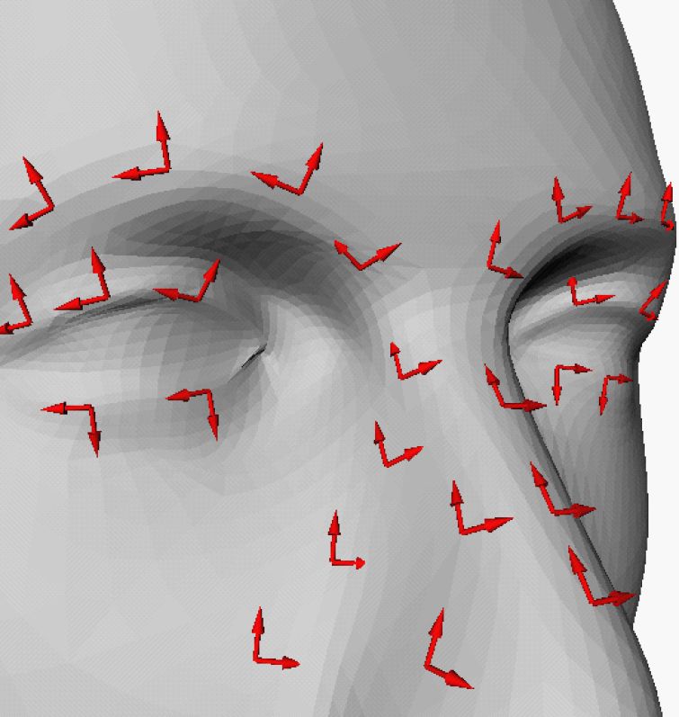
2 · Sylvain Petitjean
a need to create geometric models of existing objects. This process constitutes the ge-
ometric aspect of reverse engineering (cf. [Várady et al. 1997] for an introduction). An
important step in the reverse engineering of solid models from 3D depth maps of scanned
objects is the segmentation of the input data, i.e. the grouping of the points in the origi-
nal dataset into subsets each of which logically belong to a single primitive surface (see
Figure 1).
a. b. c.
Fig. 1. Reverse engineering of a steering arm [Thompson et al. 1999]. a. Original part. b. Sensed 3D position
points. c. Exploded view of the features making up the reverse engineered part.
• Surface reconstruction and geometry enhancement: The problem of reconstructing sur-
faces from a sparse set of unorganized points arises in various contexts such as computer
graphics, computer vision and computational chemistry (see [Mencl and Müller 1998]
for a survey of ongoing research). Most currently known methods output a polyhedral
mesh interpolating the input data ([Boissonnat and Cazals 2000] is a notable exception).
But this may not be enough. For instance, people in the CAGD community consider
computing a piecewise-linear surface from a point cloud as only a first step of a more
global process and what they mean by reconstruction is fully recovering the geomet-
ric structure of the data, i.e. the surfaces underlying the point set, be them low-degree
surfaces or more complex rational B-splines.
For other applications, a partial recovery of simple shapes (spheres, cylinders, . . . ) is
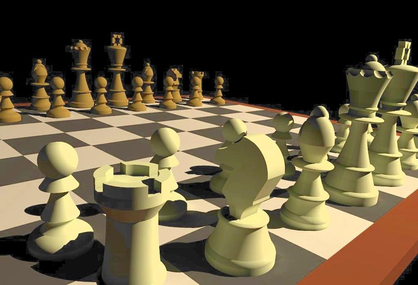
sufficient. As an example, it was recently shown in the field of global illumination that
it is both physically more accurate and computationally more efficient to render low-
degree parametric surfaces directly than to tessellate them in dozens of triangles as in
traditional radiosity approaches [Alonso et al. 2001] (see Figure 2). But since the bulk
of the models known to the computer graphics community are piecewise-linear models,
it is important to be able to recover surfaces of simple geometric type in triangulated
surfaces. This is all the more so true that most man-made objects can be modeled exactly
or at least well approximated by a small set of simple surface patches. Indeed, according
to Nourse et al. [1980], 85 percent of all mechanical pieces are well described by patches
of planes, cones, spheres and cylinders. If in addition toroidal surfaces are allowed,
then this primitive set encompasses 95 percent of conventional, unsculptured parts in
industrial environments [Requicha and Voelcker 1982].
• Model-based recognition and object registration: Model-based recognition is the task of
determining which, if any, of a given set of objects appears in a given 2D image or image
sequence. Thus, object recognition is a problem of matching models from a database
with representations of those models extracted from image data. To deal with the many
possible transformations that an object may undergo in the imaging process, a popular
ACM Computing Surveys, Vol. 2, No. 34, July 2002.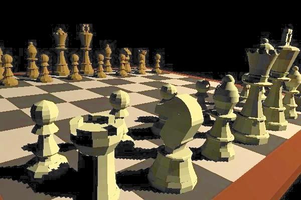
A Survey of Methods for Recovering Quadrics in Triangle Meshes                        ·      3

 a.                                                    b.

Fig. 2. Illuminating a piecewise-linear mesh (a.) and the quadrics-based model recovered (b.) [Alonso et al.
2001].

      approach is to find measurements of the object that are invariant to these types of trans-
      formations [Besl and Jain 1986]. If the objects considered are free-form and described
      by high-order surfaces, matching may prove difficult to achieve. One possible approach
      is to divide both the base models and the measured data into low-degree surface patches
      and use the component patches as features in the object recognition system [Bolle and
      Cooper 1986; Nguyen et al. 1999]. Such a strategy can also be useful to register objects
      in the input data, i.e. to estimate their pose.
• Matching overlapping range images: The data produced by laser range scanning sys-
  tems typically consists of a rectangular grid of distances from the sensor to the object
  being scanned. If more sophisticated systems are capable of digitizing some types of
  curved objects (e.g. cylindrical objects), the scanning of topologically more complex
  objects (like those having handles) cannot be accomplished directly. Clearly, multiple
  view points must be used. Matching overlapping range images is a key problem in the
  construction of CAGD models from full range images (reverse engineering) and for re-
  covering scene descriptions from multiple views in computer vision.
  To put a set of overlapping range images in a common 3D reference frame, the tradi-
  tional approach consists in first determining the motion parameters used to describe the
  correspondence between points in adjacent images and then reconstructing a compos-
  ite surface by mapping each range data point into a common reference frame [Soucy
  and Ferrie 1997; Eggert et al. 1998]. For motion parameter calculation, it is usually
  necessary to estimate local surface geometry and recover simple surface patches.
• Analytical representation of segmented volume data: The development of Magnetic Res-
  onance and Computer Tomography imaging techniques has led to the ability to create
  3D data sets and to view, for instance, areas of the human anatomy not previously reach-
  able without invasive procedures. If one is interested not just in viewing the data but
  also exploring and analyzing them (like for instance modeling the blood flow through a
  diseased artery), then tools are needed to accurately and precisely recover the shape of
  objects in an image. Analytically representing the digital shapes obtained by segmenting
  volumetric industrial or medical images can help in this respect (see, e.g., [Sanderson
  1996]).
• Surface sketching and algebraic surface design: A major task of CAGD is to automate
  the design process of such industrial objects as car parts and airplane wings, usually
  represented by smooth meshes of curves and surfaces. Ideally, one would like to po-
                                                               ACM Computing Surveys, Vol. 2, No. 34, July 2002.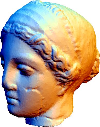
4      ·      Sylvain Petitjean

    sition a number of key points and curves and let the system infer the interpolating or
    approximating shape [Bajaj et al. 1993]. Related is interactive surface sketching, where
    free-form surfaces are created according to a sketch made by the user with the help of a
    stylus or a mouse [Sachs et al. 1991].

   While shape recovery algorithms addressing these problems have often been crafted on
a case by case basis to exploit partial structure in the data or in the problem formulation,
there are common themes to all methods. In particular, the following tasks always appear,
in one form or another: estimation (computing the local surface geometry by way of
differential parameters such as normals, curvatures, . . . ), segmentation (dividing the point
set into subsets having similar geometric characteristics), classification (deciding to which
surface type – e.g. spherical vs. cylindrical – segmented points belong) and reconstruction
(finding the surface best fitting a set of points).
   This idealized separation of the tasks is an oversimplification. For instance, differential
parameters are more reliable when estimated from a fitted surface, but reconstruction needs
segmentation to be done first and segmentation is usually driven by estimates of the cur-
vatures and other differential parameters. In the field of computer vision, researchers have
advocated carrying out the three stages of segmentation, classification and fitting simulta-
neously rather than sequentially [Besl and Jain 1988]. For the sake of clarity of exposition,
we shall however follow the natural order proposed above.
   Given a polyhedral surface as input, most shape recovery methods start by estimating
the local surface geometry at each point. The importance of such intrinsic properties such
as surface curvatures for describing shape has been recognized early [Besl and Jain 1986].
Indeed, such properties are unaffected by the choice of the coordinate system and the
particular parameterization of the surface. For all practical purposes, the local geometry at
a point of a differential surface S is well captured by a second-order surface which locally
“looks” like S. This is because differential objects like tangents, normals, curvatures and
inflections make use of first- and second-order derivatives only.
   If this initial step is more or less common to all shape recovery methods, the remaining
steps depend heavily on the class of surfaces to be looked for in the data. The search for
feature lines along which the mesh is to be segmented is intimately linked to the type of
curved surfaces one wants to recover, even though some features, like sharp edges, have to
be identified regardless of which surfaces one is after.
   In this paper, we are interested in second-order surfaces [Blinn 1997]. This class of
surfaces includes such shapes as ellipsoids, hyperboloids, cones, cylinders and paraboloids
(see Figure 3). We survey the shape recovery methods that have been specifically tailored
for extracting quadric surfaces or that can be nicely adapted to that class of surfaces. We
focus on triangulations more than on range images. Shape recovery methods developed
for data from structured light sensors such as the laser range finder or depth images from
stereo pairs (see [Arman and Aggarwal 1993] for a survey) rarely apply to triangle meshes.
Indeed, data from these techniques result in 3D points having a natural parameterization
(the one given by the grid on which the points are aligned) which is exploited by shape
extraction algorithms. For instance, Jiang and Bunke [1999] use the natural structure of
range images to perform a segmentation based on a scan-line algorithm. By contrast,
triangulated surfaces have no such natural parameterization [Stokely and Wu 1992].
   Note that we are primarily interested in extracting quadrics from discretized data com-
ing from physical objects with exactly quadric boundaries. Indeed, close studies of the
ACM Computing Surveys, Vol. 2, No. 34, July 2002.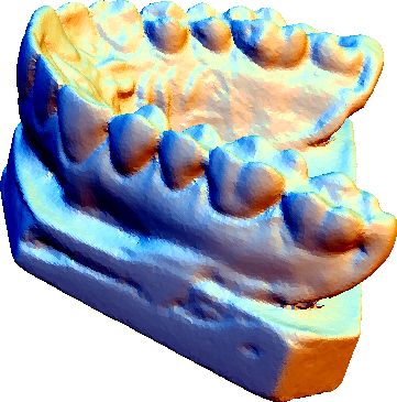
A Survey of Methods for Recovering Quadrics in Triangle Meshes · 5
1
1 1.2
0.8
0.8 1 3
0.6 0.8
0.6
0.6 2
0.4
0.4
0.2
0.4
1
0.2 0.2
0
0 0 0
-0.2 -0.2
-0.2
-0.4 -0.4 -1
-0.4
-0.6
-0.6
-0.6 -0.8 -2
-0.8
-0.8
-1
-3
-1 -1.2
-1 -1 -1
-0.8 -1 -1
-0.4 -0.4 -3
-1.6 -2
0 0 -1 -1.2
0.2 0.2 0
-0.8 0 -0.8-1 -1
-3
0.4 0.4 -0.4 0.5 -0.4 0 -2
0
0.6 0.6 0.2
0 0.40.2 1
0
-1
0.8 0.8 0.5
0.4 1 0.80.6 2 1
11 0.6 1.2 1 3 2
1
0.8
1.61.4 3
1
0.8
1 0.6
0.4
1 1
0.5 0.2
0.8
0.5 0
0.6
0 -0.2
0.4
0
-0.4
0.2
-0.5
-0.6
-0.5 0
-1 -0.8
-1
-1
-1 -1 -1 -1
0 0 -0.5
-0.5 0.5 0
-1 0 0.5
1 0.5
-0.6 0.5 0
0 1.5 11
1
0 2
0.5 0.2 1.5
-0.8 -1
-0.2 -0.4 -0.6
0.4
0.8 1 0.4 0.2 0
1 1 1 0.8 0.6
Fig. 3. Some instances of quadric surfaces. First row: ellipsoid, cone, hyperboloid of one sheet, hyperboloid of
two sheets. Second row: elliptic cylinder, parabolic cylinder, paraboloid, hyperbolic paraboloid.
problem have led to the conclusion that implicit quadrics are inappropriate for approxi-
mating arbitrary data [Moore and Warren 1991; Sapidis and Besl 1995]. In other words,
quadric-based segmentation fails to produce acceptable results when the data originate
from arbitrarily shaped curved objects (for instance the final regions may be small and
have many gaps).
The organization of the paper follows the succession of tasks introduced above. After
recalling some notions of differential geometry (Section 2), we review in Section 3 some
of the best methods for estimating local surface geometry, i.e. essentially normal and prin-
cipal curvatures. After differential parameters have been estimated at each data point, we
examine in Section 4 how they can be made consistent over the entire triangulation. Then
we move on to the segmentation and classification tasks in Section 5. Finally, Section 6 is
devoted to the final reconstruction and fitting step, before concluding.
2. DIFFERENTIAL GEOMETRY: A FLAVOR
As already indicated, differential geometry provides a convenient basis for describing the
local behavior of a surface in the vicinity of some particular point. It has been widely used
in computer vision and object recognition as a tool for describing surfaces. Differential
geometry parameters are also essential elements of shape recovery methods. Indeed, many
methods for estimating the local geometry of a surface approximating a set of points start
by computing some differential properties of that surface.
In this section, we recall a few key notions of differential geometry (the interested reader
should refer to [do Carmo 1976] for proofs and additional details).
In what follows, S is assumed to be a surface embedded in R3 , described by an arbitrary
parameterization of two variables X(u, v) and smooth in the vicinity of point p.
2.1 Fundamental forms and shape operator
Up to orientation of the surface, the unit normal n to S at p is given by:
Xu × Xv
n= ,
kXu × Xv k
ACM Computing Surveys, Vol. 2, No. 34, July 2002.6 · Sylvain Petitjean
where subscripts indicate partial derivatives and × denotes the cross product. The first and
second fundamental forms of S are defined as
I(u, v, du, dv) = dX · dX = duT Gdu, II(u, v, du, dv) = −dX · dn = duT Ddu,
where du = (du, dv)T and
! !
Xu · X u X u · X v n · Xuu n · Xuv
G= , D= .
Xu · Xv Xv · Xv n · Xuv n · Xvv
The first fundamental form measures the small amount of movement on the surface for a
given small movement in the space of the parameters (u, v). It is invariant to surface pa-
rameterization changes and to translations and rotations of the surface. It does not depend
on the way the surface S is embedded in 3D space, and is therefore an intrinsic property
of the surface. By contrast, the second fundamental form, which measures the change in
the unit normal for a movement in parameter space, depends on the embedding of S and is
thus an extrinsic property of the surface.
For t a vector tangent to S at p, i.e. t · n = 0, define the shape operator or Weingarten
map β by
β(t) = −∇t n,
where ∇t n is the directional derivative of n in the direction t (also called covariant deriva-
tive of n by t):
n(p + τ t) − n(p)
(∇t n)(p) = lim .
τ →0 τ
The shape operator is a linear operator Γp → Γp , where Γp is the space tangent to S at p.
In matrix form, it writes down as
β(t) = G −1 Dt.
Let S be the matrix G −1 D. One can view the matrix S as the entity that determines surface
shape by relating the intrinsic geometry of the surface to the Euclidean geometry of 3D
space. It is a generalization of the curvature of plane curves.
2.2 Principal curvatures and directions
Let t again be a tangent vector at p. The normal curvature of S at p in the direction t is
the curvature of the plane curve formed by the intersection of the plane defined by t and n
with the surface. It is defined by:
β(t) · t
κn (t) = .
ktk2
The principal curvatures κ1 and κ2 at p are the maximum and minimum values of κn
respectively. The unit directions e1 and e2 for which these values are reached are called
the principal directions of S at p. κ1 and κ2 are the eigenvalues of the shape operator. e1
and e2 are the corresponding eigenvectors. With n, they form an orthonormal frame at p,
the principal coordinate frame. This frame is well-defined except at umbilic points, which
are points at which the principal curvatures are equal.
If θ is the angle from e1 to t in the orientation of the tangent plane to S at p, the
expression of the second fundamental form in the basis {e1 , e2 } is:
κn (θ) = κ1 cos2 θ + κ2 sin2 θ.
ACM Computing Surveys, Vol. 2, No. 34, July 2002.A Survey of Methods for Recovering Quadrics in Triangle Meshes · 7
It is known as the Euler formula. Also, if C is a curve lying on S of curvature κ, N its
normal vector and ϕ the angle between n and N at p, then the normal curvature of S at p
in the direction of the tangent t to C is
κn = κ cos ϕ.
This is Meusnier’s theorem.
Useful shape descriptors can be derived from the principal curvatures. The mean curva-
ture H is defined as the average of the normal curvatures:
Z 2π
1
H= κn (θ) dθ. (1)
2π 0
Using the Euler formula, this reduces to H = (κ1 + κ2 )/2. The Gaussian curvature K is
defined as the product of the two principal curvatures: K = κ1 κ2 . In other words, K is the
determinant of S and H is its half-trace. A point of the surface is called elliptic if K > 0,
hyperbolic if K < 0, parabolic if K = 0 and H 6= 0, and planar if K = H = 0.
2.3 Principal quadric
A neighborhood of a smooth point p on S can be represented in the form z = h(x, y),
where p is the origin of the local coordinate frame and the z axis is directed by the normal
n at p. h is a differentiable function and by Taylor’s expansion at p, we have:
1 p 2 R(x, y)
h(x, y) = (h x + 2hp p 2
xy xy + hyy y ) + R(x, y) with lim = 0,
2 xx (x,y)→(0,0) x2 + y 2
where hp p p
xx means hxx evaluated at p. (Note that hx = hy = 0 because n is along the z
axis.) The quadratic surface Q defined as the zero-set of the equation
1 p 2
z= (h x + 2hp p 2
xy xy + hyy y )
2 xx
approximates S up to order 2 and is called the principal or osculating quadric of S at p.
At a hyperbolic point, Q is a hyperbolic paraboloid. At an elliptic point, it is an elliptic
paraboloid. At a parabolic point, it is a parabolic cylinder. And at a planar point, it is a
plane.
Locally, S can be parameterized by X(x, y) = (x, y, h(x, y))T with n = (0, 0, 1)T . In
turn, this means that
p
hxx hp
p
hxx hp
1 0 xy xy
G= , D= , S = .
0 1 hp p
xy hyy hp p
xy hyy
In other words, since κ1 and κ2 are the eigenvalues of S, the principal quadric has the
following equation in the principal coordinate frame:
1
z= (κ1 x2 + κ2 y 2 ).
2
The principal quadric thus encodes all the relevant differential information of the surface
S at p.
3. LOCAL SURFACE GEOMETRY ESTIMATION
Estimating the local surface geometry at a vertex p of a piecewise-linear surface amounts
to computing what Sander and Zucker called the augmented Darboux frame [Sander and
ACM Computing Surveys, Vol. 2, No. 34, July 2002.8 · Sylvain Petitjean
Zucker 1990] at p, i.e.
∆p = (p, e1 , e2 , n, κ1 , κ2 ).
Computing Darboux frames is a prerequisite to most segmentation and shape recovery
methods. It is also a key ingredient of surface re-parameterization, geometry-based subdi-
vision, mesh simplification [Heckbert and Garland 1999] and surface denoising [Desbrun
et al. 1999] algorithms. In fact, many surface-oriented applications require an approxima-
tion of the first- and second-order differential properties of a piecewise-linear surface with
as much accuracy as possible.
Estimating the Darboux frames of a subjacent, unknown, piecewise-smooth surface from
a polyhedral approximation is difficult because of the inherently discrete nature of the data.
In addition, differential quantities such as principal curvatures and directions, involving
second-order partial derivatives, are very sensitive to measurement and quantization errors.
In practice, this means that estimates computed on a local basis must be improved in a
second global stage of processing (Section 4).
This section examines some of the most powerful methods for locally estimating the
differential properties of a triangle mesh1 . There are three ways to take the information
provided by the surface into account:
1. forget the point-to-point connectivity and estimate local geometry using only the 3D
vertex set;
2. use the mesh connectivity as a purely topological attribute;
3. interpolate the data using the mesh structure.
We believe the two extremes (1. and 3.) are poor ways of approaching the problem con-
sidered. Indeed, methods of the first kind (see, e.g., [Várady et al. 1998]) may have a hard
time defining surface orientation and normal in regions where the vertex set is not dense
enough, while methods of the third kind need to build an interpolating mesh with high-
order continuity (as in [Samson and Mallet 1997], where Bézier patches are used to build
a mesh with G2 continuity), which is hard to achieve. Consequently, this paper focuses on
methods of the second type only.
In many methods, vertex normal and principal directions are computed in a single pass.
Some iterative methods, however, need an initial estimate of the normal. So we start by
indicating how vertex normal can be estimated based on the normals of the incident faces
(§ 3.1). We then examine how the principal quadric – and thus the Darboux frame – can be
directly estimated by local surface fitting (§ 3.2). We next present some methods based on
interpretations in the “discrete” domain of results of differential geometry (§ 3.3), before
turning our attention to techniques having a signal processing flavor, which are largely
immune to the inherent difficulties of computing differential quantities of quantized objects
(§ 3.4). We conclude by saying a word on the comparison between these different methods
(§ 3.5).
In what follows, T is assumed to be an oriented and consistent triangulated surface with
boundary [Foley et al. 1992]. In other words, neighboring triangles have their normals
pointing to the same side of the surface. For p a vertex of T , we call 1-ring neighborhood
1 Thoughwe use triangulations for our presentation, some of the methods presented below are also applicable to
more general piecewise-linear surfaces.
ACM Computing Surveys, Vol. 2, No. 34, July 2002.A Survey of Methods for Recovering Quadrics in Triangle Meshes · 9
of p the set of triangles incident to p. We denote by N (p) the set of 1-ring neighbor
vertices pi of p and m the cardinal of N (p) (the valence of p).
3.1 Vertex normal estimate
It is commonly suggested to compute the normal at a vertex p of a piecewise-linear surface
as a (possibly weighted) average of the normals of the faces adjacent to p, i.e.
Pm
wi ni
n = Pi=1 m ,
k i=1 wi ni k
where the ni are the unit normals to the triangles in the 1-ring neighborhood of p.
Various kinds of averages have been proposed in the literature, in particular arithmetic,
area-weighted and angle-weighted averages [Meek and Walton 2000]. Gouraud [1971]
takes wi = 1, i.e. he considers unweighted averages. Obviously, this definition depends
heavily on the local meshing around p and two different meshings may result in two differ-
ent normals. Arguing that the normal vector should be independent of the shape or length
of the adjacent faces, Thürmer and Wüthrich [1998] propose an angle-weighted average,
i.e. wi = θi , where θi is the angle of the i-th face at vertex p (see Figure 7.c). However,
this estimate may be worse than the unweighted average when all vertices are on a smooth
surface. Max [1999] derives weights which give the exact normal at p if the triangulation
is a (possibly irregular) tessellation of a sphere, i.e.
sin θi
wi = .
kppi k kppi+1 k
Others have proposed taking weights proportional to the areas (or the areas of subregions)
of the incident faces. For instance, to stay in line with what is advocated in [Desbrun et al.
2000], one can use weights equal to the areas of the local barycentric cells, as in Figure 7.a.
3.2 Fitting for principal quadric estimation
To robustly estimate the local surface geometry of T , a good start may be to compute the
principal quadric at each vertex p. We show in this section how the principal quadric can be
directly estimated by local surface fitting. Our exposition largely follows that of [McIvor
and Valkenburg 1997].
Note that since the differential parameters to be estimated are functions of derivatives
up to second order, it is intuitively sufficient to fit second-order surfaces. This is confirmed
by experimental results. For instance, Krsek et al. [1998] report little advantage working
with third- and fourth-order surfaces over second-order surfaces.
3.2.1 General approach. Let xw be a point with coordinates expressed in the global
(world) coordinate frame in which the data is obtained. Let x = (x, y, z)T be the co-
ordinates of that point in the principal coordinate frame associated with a given point p.
Then
x = R(xw − pw ),
where R is a rotation matrix called the attitude matrix.
Estimating all the parameters of the principal quadric at p at the same time may not
be easy. In general, this task is separated into two subproblems: estimating the surface
normal and estimating the principal directions. This is achieved by making use of a rotated
ACM Computing Surveys, Vol. 2, No. 34, July 2002.10 · Sylvain Petitjean
principal quadric, which is the principal quadric expressed in a coordinate frame x0 =
(x0 , y 0 , z 0 )T related to the principal frame by a rotation about the surface normal:
cos α sin α 0
x = − sin α cos α 0 x0 . (2)
0 0 1
The rotated principal quadric has the form
2 2
z 0 = a0 x0 + b0 x0 y 0 + c0 y 0 (3)
and the associated shape operator matrix is
0 0
2a b
S= .
b0 2c0
Its eigenvalues and eigenvectors are the principal curvatures and directions. A straightfor-
ward calculation gives:
q q
0 0 0 0
κ1 = a + c + (a − c ) + b , κ2 = a + c − (a0 − c0 )2 + b0 2 ,
0 0 2 0 2
(4)
1 2
α = atan2(b0 , a0 − c0 ), K = 4a0 c0 − b0 , H = a0 + c0 .
2
The transformation from the world coordinate frame to a rotated principal frame is then
x0 = R0 (xw − pw ). (5)
0 T
One useful rotated principal frame is defined by choosing R = (r1 , r2 , r3 ) as follows:
(I − nnT )i
r3 = n, r1 = , r2 = r3 × r1 , (6)
k(I − nnT )ik
where i is along the first axis in the global coordinate frame and I is the identity matrix. In
other words, rotation R0 aligns x0 with the projection of xw onto the tangent plane defined
by n.
A typical method (e.g. [Sander and Zucker 1990; Stokely and Wu 1992; Ferrie et al.
1993; Hamann 1993]) for estimating the principal quadric then goes as follows:
1. Estimate the surface normal at p with one of the definitions of § 3.1 or by finding the
plane best fitting p and its 1-ring neighbors.
2. Construct the rotation matrix R0 using (6).
3. Map the world data to the rotated principal frame with (5).
4. Fit the mapped data to the rotated principal quadric (3), and solve the resulting system,
giving a0 , b0 , c0 .
5. Compute κ1 , κ2 , α from a0 , b0 , c0 using (4).
6. Estimate the attitude matrix by concatenating the transformations (2) and R0 .
The coefficients of the rotated principal quadric (Step 4) are obtained by solving the
following over-determined system of linear equations:
2 2
x1 y1 x1 y1 a0 z1
.. .. .. b0 = .. .
. . . .
0
2 2
xn yn xn yn c zn
ACM Computing Surveys, Vol. 2, No. 34, July 2002.A Survey of Methods for Recovering Quadrics in Triangle Meshes · 11
This system can be solved using a least-squares method.
3.2.2 Improvements. Several improvements can be made to this basic principal quadric
estimation scheme.
First, it is clear that with the above method, the estimation of the Darboux frame relies
heavily on the accuracy of the estimation of the surface normal. Inaccuracies in the sur-
face normal estimate can be allowed by fitting an extended quadric instead of the rotated
principal quadric. Compared to the basic method described above, Steps 1-3 and 6 are
unchanged and Steps 4-5 now become [McIvor and Valkenburg 1997]:
4. Fit the mapped data to the extended quadric
ẑ = a0 x̂2 + b0 x̂ŷ + c0 ŷ 2 + d0 x̂ + e0 ŷ,
giving a new estimate of the surface normal at p:
(−d0 , −e0 , 1)T
n= .
1 + d0 2 + e0 2
From this, the rotation needed to align ẑ with n can be calculated. The data is mapped
into this new coordinate frame and a new quadric fitted. The iteration stops when the
incremental change in the direction of the normal falls below some tolerance level.
5. Estimate the differential parameters as follows:
2 2 2
4a0 c0 − b0 a0 + c0 + a0 e0 + c0 d0 − b0 d0 e0
K= , H= ,
(1 + d0 2 + e0 2 )2 (1 + d0 2 + e0 2 )3/2
where a0 , b0 , c0 , d0 , e0 are the parameters of the last quadric fitted.
An iterative method similar to this one is described in [Fitzgibbon and Fisher 1993].
A further improvement is obtained by adding a zero-order term to the quadric to be
fitted. This is the same as removing the constraint that the point p has to lie on the fitted
surface [McIvor and Valkenburg 1997].
An alternative to the linear iterative scheme above is the following 7-dimensional non-
linear optimization problem [McIvor and Valkenburg 1997]:
min z̃ − (a0 x̃2 + b0 x̃ỹ + c0 ỹ 2 + f 0 ) , (7)
R̃,a0 ,b0 ,c0 ,f 0
where x̃ = (x̃, ỹ, z̃)T = R̃(x̃w − p̃w ), where the parameter f 0 is added to accommodate
noise in the data at p. Note that Eq. (7) has 4 linear (a0 , b0 , c0 , f 0 ) and 3 non-linear (the
three Euler angles of R̃) parameters, so special techniques for separable least-squares can
be used.
3.3 Surface description from differential geometry
Apart from the above fitting techniques, many methods have been proposed for estimating
local surface geometry based on results from differential geometry. We elaborate here on
some of the most interesting ones.
3.3.1 Approximation by curves. Fast methods for estimating differential parameters
result from approximating planar sections of the surface by simple curves.
One such method is the circle fitting algorithm [Martin 1998]. Let p be the point at
which principal curvatures are to be estimated. The algorithm roughly goes as follows:
ACM Computing Surveys, Vol. 2, No. 34, July 2002.12 · Sylvain Petitjean
• Choose triples of points, each having p and two other vertices in the 1-ring neighborhood
of p (one on each side of p) in common. Let l be the number of such triples (l is
necessarily ≥ 3).
• Compute the circle Cj interpolating each triple, j = 1, . . . , l. Let kj be the curvature of
Cj (i.e. the inverse of the radius of Cj ) and nj the normal of the plane containing Cj .
• For each Cj , the line through p and tangent to Cj (let tj be its direction) can be con-
sidered as being tangent to the surface. The normal n at p is perpendicular to each such
tangent line. Estimates of this normal are obtained either by taking tangents tj pairwise
and computing the average of the cross products, or by finding the plane P best fitting
all tangents (least-squares fit).
• Let t0j be the projection of tj on P , i.e.
t0j = tj − (tj · n)n.
Each Cj can be considered as being contained in the surface. So the normal curvature
κn (t0j ) of the surface at p in the direction t0j is, by Meusnier’s theorem, κn (t0j ) =
kj cos ϕj , where ϕj is the angle between n and nj .
• Let t0 be an arbitrary reference direction in P and θ0 the angle between the first principal
direction and t0 . Let θj be the angle between t0j and t0 . Then, using the Euler formula,
we are left with a set of equations
κn (t0j ) = κ1 cos2 (θj − θ0 ) + κ2 sin2 (θj − θ0 )
in the variables κ1 , κ2 and θ0 which can be solved using a least-squares method. Rotat-
ing t0 by an angle of θ0 and θ0 + π2 then gives e1 and e2 respectively.
A closely related method is the quadratic complexity algorithm of [Chen and Schmitt
1992], which is also based on fitting circles to triples of points. However, given the point p
at which curvature is to be measured and one of its neighbors pi , not all triples (p, pi , pj )
with pj on the opposite side of p are taken into account. The strategy is to define a measure
of geometric oppositeness M = (p − pi ) · (pj − p), compute M for all possible triples,
sort the results in decreasing order and keep only the triples corresponding to the first l
values of M (there are at least 3). This way, the curves C interpolating the retained triples
are close to the normal section and the angle ϕ between n and the normal to the plane
containing C is close to 0 or π. Since Meusnier’s theorem involves cos ϕ, this limits the
effects of computation error for ϕ and allows for some noise in vertex position to be taken
into account.
3.3.2 Surface normal changes. Another method considering local approximation by
circular arcs is presented in [Karbacher and Häusler 1998]. Assume that the sampling
density is high enough so as to neglect variations of surface curvature between adjacent
sample points. Let ni , nj be the normals estimated at neighboring vertices pi , pj (again
with any of the definitions of § 3.1). Consider the circle Sij going through pi and pj and
tangent to the surface at these points (i.e. Sij is orthogonal to ni at pi and to nj and pj ).
Let pij be the center of Sij and dij the distance between the two vertices (Figure 4). Then
the curvature of Sij can be estimated as:
∠pi pij pj
cij ≈ ± ≈ ± arccos (ni · nj ),
dij
ACM Computing Surveys, Vol. 2, No. 34, July 2002.A Survey of Methods for Recovering Quadrics in Triangle Meshes · 13
where cij > 0 for a concave area and cij < 0 for a convex area. The principal curvatures
at pi are then estimated as the extrema of cij over all vertices pj neighboring pi :
κ1 ≈ max (cij ), κ2 ≈ min (cij ).
j j
Knowing κ1 , κ2 and a set of normal curvatures at pi (the cij ) in several different directions,
one can deduce the principal directions by applying Meusnier’s theorem and solving the
resulting system.
ni Sij
nj
dij pj
pi
pij
Fig. 4. Approximating the surface by a mesh of circular arcs.
Other authors have considered estimating differential parameters as functions of surface
normal changes. The method of [Hoschek et al. 1998] relies on an estimate of the angular
variation of the normal close to a particular vertex, while [Krsek et al. 1998] discuss the
use of the angular deficit at a vertex as a measure of the curvature. Unfortunately, these
two methods may not get the magnitude of the curvature right and they may have troubles
with noisy data.
Now consider the following general approach [Flynn and Jain 1989]. For any pair of
triangles which share an edge pi pj , compute the curvature of the sphere passing through
the four vertices involved. (Set this curvature to zero if the four points are coplanar.) The
sign of the curvature is taken to be positive if the center of the sphere is on the same side of
the surface as the normals at pi and pj , negative otherwise. An estimated curvature value
for a given triangle is then taken as the average of the curvatures obtained when it is paired
with each of the triangles with which it shares an edge. However, results can be affected
by noise in the data.
To compensate for the effect of errors in the positions of triangle vertices, Sacchi et
al. [1999] proposed the following algorithm. First, compute an interpolated normal at each
vertex of the triangulation as the weighted average of the normals of the incident triangles,
with weights equal to the areas of the triangles. Take as compensated normal of a triangle
the weighted average of the three interpolated normals at the vertices of the triangle, using
as weight, for each vertex, the sum of the areas of the incident faces. Similarly, define
the compensated center of each triangle as the weighted average of the vertices using the
same weights as before. For a pair of triangles with compensated normals n1 and n2 and
compensated centers c1 and c2 , take as estimate of the curvature of their common edge
kn1 × n2 k
c12 = .
kc1 − c2 k
For a given triangle, we thus obtain three curvature values. Pairing the compensated nor-
mal of the triangle with the interpolated normals at the three vertices of the triangle and
ACM Computing Surveys, Vol. 2, No. 34, July 2002.14 · Sylvain Petitjean
applying Meusnier’s theorem gives three additional curvature values. The estimated mean
curvature of a triangle is then taken as the average of the maximum and the minimum of
the six curvature measures.
Application of this curvature estimation method on the a surface representing a technical
device is shown on Figure 5.
Fig. 5. From left to right: a triangle mesh, regions of high mean curvature (in blue) and identification of planar
regions [Sacchi et al. 1999].
3.3.3 Tensor of curvature. Using the notations of Section 2, consider the following
symmetric 3 × 3 matrix
Z π
1
M= κn (t) ttT dθ,
2π −π
where t = cos θe1 + sin θe2 . Taubin [1995b] proves that M can be factored as follows:
T m1 0
M = E12 E ,
0 m2 12
where E12 = [e1 , e2 ] is the 3 × 2 matrix constructed by concatenating the column vectors
e1 and e2 and
κ1 = 3m1 − m2 , κ2 = 3m2 − m1 . (8)
That is, the eigenvectors of M are 0, m1 , m2 and the corresponding eigenvectors are
n, e1 , e2 . In other words, an estimation of the tensor of curvature (i.e. the map which
assigns each point p of S to κn (t), the normal curvature of S at p in the direction of the
unit vector t) follows from an estimation of M.
Taubin [1995b] proposes the following algorithm, which is both linear in time and space,
to perform this estimation. Let p be a vertex of T , N (p) its set of 1-ring neighbor vertices.
Let n be an estimate of the unit normal at p. Then the matrix M can be approximated as
follows:
X
Mp = wi κin ti tTi ,
pi ∈N (p)
where the weight wi is chosen to be proportional to the sum of the surface areas of the
triangles incident to both p and pi (there is only one
P such triangle if p and pi are both on
the boundary of T , two otherwise) and such that pi ∈N (p) wi = 1, ti is the normalized
projection of pi − p onto the tangent plane hni⊥ and κin is an estimate of the normal
ACM Computing Surveys, Vol. 2, No. 34, July 2002.A Survey of Methods for Recovering Quadrics in Triangle Meshes · 15
curvature in the direction ti :
(pi − p) − [(pi − p) · n]n 2n · (pi − p)
ti = , κin = .
k(pi − p) − [(pi − p) · n]nk kpi − pk2
Justification for this approximation of κn is best explained with the help of Figure 6: the
radius Ri of the osculating circle through p and pi must be such that there is a right angle
at vertex pi :
(p − pi ) · (p − pi − 2Ri n) = 0.
Since κin
is just the inverse of Ri , the approximation follows2 . (Note that there is an error
in the formula given by [Taubin 1995b].)
n
p
p
i
Ri
Fig. 6. Osculating circle for edge ppi .
By construction, n is an eigenvector of Mp associated with the eigenvalue 0. To com-
pute the remaining eigenpairs, Mp is restricted to the tangent plane hni⊥ using a House-
holder transformation and then diagonalized. Let i = (1, 0, 0)T be the first coordinate
vector and let
i + εn
Wp = , Qp = I − 2Wp WpT ,
ki + εnk
where ε = −1 if ki − nk > ki + nk, ε = 1 otherwise. Qp is the Householder matrix, an
orthogonal matrix having εn as its first column. The other two columns (ẽ1 and ẽ2 ) define
an orthonormal basis of the tangent space. Thus:
0 0 0
QTp Mp Qp = 0 m̃1 m̃3 .
0 m̃3 m̃2
The 2 × 2 nonzero minor can be diagonalized, given an angle η such that
e1 = cos η ẽ1 − sin η ẽ2 , e2 = sin η ẽ1 + cos η ẽ2
2 Thisformula leads to a straightforward calculation of H and K as follows [Watanabe and Belyaev 2000].
Applying a trapezoid approximation to Eq. (1) yields:
Z 2π
1 θ + θ
m 1
θ
m−1 + θm
H= κn (θ) dθ = κn + · · · + κn ,
2π 0 2 2
where θi is the angle of the i-face at p. This gives an estimate of H. A similar calculation leads to:
Z 2π
1 3H 2 − K
κ2n (θ) dθ = .
2π 0 2
Applying again a trapezoid rule gives an estimate of K.
ACM Computing Surveys, Vol. 2, No. 34, July 2002.16 · Sylvain Petitjean
are the remaining eigenvectors of Mp , i.e., the estimates of the principal directions of the
surface at p. The principal curvatures are obtained from the two corresponding eigenvalues
of Mp using Eq. (8).
Note that the above method, even though it was described for a surface triangulation,
can be extended to a discrete set of points, as recently proposed by Gopi et al. [2000] in
the context of surface reconstruction.
3.3.4 Spatial averages and 1-ring patches. Recently, Desbrun et al. [2000] have ar-
gued that the best way of extending to discrete meshes the definitions of differential quan-
tities in the continuous case is by computing spatial averages around vertices. For instance,
the average Gaussian curvature at vertex p of T should be defined in its discrete form as:
ZZ
1
K(p) = K dA,
A
A
for A a properly chosen area around p. The authors show that strong analogies between
the continuous and the discrete case are obtained by restricting the averaging domain at
vertex p to a family of special regions AM (called finite volumes) contained within the
1-ring neighborhood of p, with piecewise-linear boundaries crossing the mesh edges at
their midpoints. Two main types of finite volumes are used. In the first, the point inside
each triangle of the 1-ring neighborhood of p is the barycenter of the triangle (Figure 7.a).
In the second, this inside point is the circumcenter of the triangle and the finite volume is
recognized as the local Voronoi cell (Figure 7.b).
p
p p p
θi pi+1
αi βi
pi pi
a. b. c. d.
Fig. 7. Local regions around a vertex [Desbrun et al. 2000]. a. Finite volume region using barycentric cells. b.
Local region using Voronoi cells. c. External angles of a Voronoi region. d. 1-ring neighbors and angles opposite
to an edge.
A discrete equivalent of the Gaussian curvature is obtained by applying the Gauss-
Bonnet theorem to the finite volume AM . Roughly RR speaking, this theorem says that given
a region R of a surface, the integral curvature R K dA measures the solid angle filled
by all unit normals to R, translated to one point. In the discrete domain, this means that
ZZ X
K dA = 2π − θi ,
AM pi ∈N (p)
where θi is the angle of the i-th face at vertex p (see Figure 7.c). This formula holds for
any surface patch within the 1-ring neighborhood whose boundary crosses the edges at their
midpoint. But one finite volume region must be chosen to provide an accurate estimate of
the spatial average. Desbrun et al. [2000] show that the Voronoi cells provide provably
ACM Computing Surveys, Vol. 2, No. 34, July 2002.A Survey of Methods for Recovering Quadrics in Triangle Meshes · 17
tight error bounds under mild assumptions of smoothness. If the 1-ring neighborhood of p
is made only of non-obtuse triangles, then the local patch has area
1 X
AVoronoi = (cot αi + cot βi )kpi − pk2 .
8
pi ∈N (p)
where αi and βi are the two angles opposite to the edge ppi as depicted in Figure 7.d. To
ensure a perfect tiling of the triangulation T and an optimal accuracy in the presence of
obtuse triangles in the 1-ring neighborhood, the authors advocate the use of mixed areas:
if a triangle is obtuse, take its barycenter as inside point; otherwise, take its circumcenter.
Denoting the area of the corresponding local patch by AMixed , an estimate of the Gaussian
curvature at p is:
1 X
K(p) = 2π − θi .
AMixed
pi ∈N (p)
Resorting to the Gauss-Bonnet theorem to find a discrete equivalent of the Gaussian curva-
ture is not new and has been proposed in the past notably in [Lin and Perry 1982; Pinkall
and Polthier 1993; Alboul and van Damme 1996]. For instance, Lin and Perry [1982]
proposed to use the following as approximation of the Gaussian curvature:
3 X
K(p) = 2π − θi ,
A
pi ∈N (p)
where A is the total area of the triangles in the 1-ring neighborhood of p.
To compute estimates of the mean curvature and vertex normal at p, the authors intro-
duce the Laplace-Beltrami operator K. On a piecewise-smooth surface S, this operator
maps a point p to the vector K(p) = 2Hp np . On a triangulation T , the integral of the
Laplace-Beltrami operator over the finite volume AM can be transformed into a line inte-
gral over the boundary of the finite volume. Computing this line integral gives
ZZ
1 X
K dA = (cot αi + cot βi )(pi − p).
2
AM pi ∈N (p)
As before, this expression holds even for 1-ring neighborhoods with obtuse triangles. To
provide an estimate of the Laplace-Beltrami operator at p, the mixed area is chosen:
1 X
K(p) = (cot αi + cot βi )(pi − p).
2AMixed
pi ∈N (p)
This vector, after normalization, provides a reasonable estimate of the vertex normal at p.
As for the mean curvature, it can be estimated by taking half of the magnitude of K(p).
When the mean curvature at p is zero, the vertex normal is obtained by averaging the 1-ring
face normal vectors (as in § 3.1).
The mean quadrature has an interesting interpretation as a quadrature of the integral of
Eq. (1):
X
H(p) = wi κin ,
pi ∈N (p)
where κinis an estimate of the normal curvature along the edge ppi (the same approxi-
mation used in [Taubin 1995b] in the estimation of the tensor of curvature) and the wi are
ACM Computing Surveys, Vol. 2, No. 34, July 2002.18 · Sylvain Petitjean
weights which sum to one for each p having no obtuse triangle in its 1-ring neighborhood:
2n · (pi − p) 1
κin = , wi = (cot αi + cot βi )kpi − pk2 .
kpi − pk2 8AMixed
To determine the principal directions, the idea is to use the κin as samples of the 2 × 2
curvature tensor S. In other words, the goal is to find S satisfying
dTi Sdi = κin , i = 1, . . . , m,
where di is the unit direction in the tangent plane of the edge ppi :
(pi − p) − [(pi − p) · n]n
di,j = .
k(pi − p) − [(pi − p) · n]nk
A least-squares approximation of S is found by minimizing the error E
X
E(S) = wi dTi Sdi − κin ,
i
subject to the constraints that the determinant of S is K(p) and its trace is 2H(p). The
eigenvectors of S then give estimates of the principal directions at p. An illustration is
given in Figure 8.
Fig. 8. Principal directions on a triangle mesh [Desbrun et al. 2000].
A different discrete formulation of the mean curvature is given in [Alboul and van
Damme 1996]. Using Eq. (1) and the Euler formula, it is a simple matter to see that at
any point of a piecewise-smooth surface S the mean curvature is the half-sum of the nor-
mal curvatures in any two orthogonal directions:
1
H= κn (t) + κn (n × t) .
2
This formula can be applied to a triangulation T . For a point on an edge e, choose as
one direction the direction along this edge and the orthogonal direction ⊥e . The curve
defined by e is a straight line, so its curvature is zero. As for the curve defined by ⊥e , the
equivalent of its curvature is the angle between the plane normals of the faces adjacent to
ACM Computing Surveys, Vol. 2, No. 34, July 2002.A Survey of Methods for Recovering Quadrics in Triangle Meshes · 19
e. The discrete mean curvature H(e) of e is thus one-half of this angle. For a domain U ,
the mean curvature is then:
X
H(U ) = H(e) length(e ∩ U ).
edge e⊂U
The ratio of H(U ) to the area of U gives an estimate of the average mean curvature over
the part of T which corresponds to U . Using the notations above, and taking U = AMixed ,
this gives another estimate of the mean curvature at p:
1 X
H(p) = kpi − pk ϕi ,
4AMixed
pi ∈N (p)
where ϕi is the dihedral angle between the two triangles meeting along the edge ppi .
3.4 Covariance matrices
Many of the original methods for measuring surface normals and curvature at points of a
range image used derivatives estimates which may not be robust under additive noise. In
addition, the image considered may not have adequate “smoothness” to support the use
of differential operators. This led several authors to explore an alternate signal processing
basis for computing local shape measures, using covariance matrices [Liang and Todhunter
1990; Berkmann and Caelli 1994]. The main advantage of this covariance approach is that
it provides ideal ways of treating signals embedded in additive Gaussian or white noise.
The covariance matrices method can be easily adapted to triangulations. Let again the
vertices pi be the 1-ring neighbors of p. Define the first-order, 3 × 3, surface covariance
matrix at p as:
m
1 X
CI = (pi − p̄) (pi − p̄)T , (9)
m i=1
1
Pm
where p̄ = m i=1 pi is the mean position vector. This matrix may be seen as a discrete
equivalent of the first fundamental form matrix G. Two of its eigenvectors (t1 and t2 )
define the plane which minimizes, in the least-squares sense, the orthogonal distance from
all points to that plane. As originally proposed in [Liang and Todhunter 1990], this plane
is a reasonable approximation to the surface tangent plane at p. Consequently, the other
eigenvector forms the equivalent of the surface normal n.
An analogous definition of the second fundamental form matrix follows by projecting
the difference vector that points from p to pi onto the “tangent plane” as determined by (9)
and weighting the resulting vector by a measure of the orthogonal distance from point pi
to the “tangent plane” [Berkmann and Caelli 1994]:
m
1 X
CII = (yi − ȳ) (yi − ȳ)T ,
m i=1
where
h i (p − p) · t
i 1
yi = (pi − p) · n ,
(pi − p) · t2
The eigenvectors of the 2 × 2 matrix CII can be considered as estimates of the principal
directions at p.
ACM Computing Surveys, Vol. 2, No. 34, July 2002.20 · Sylvain Petitjean
There are alternate ways of computing principal directions. They can for instance be
estimated by calculating the covariance matrix of a certain normal map [Liang and Tod-
hunter 1990]. Also, since they lie on the tangent plane anyway, they can be found as the
0
eigenvectors of a 2×2 covariance matrix CII built on the projections of the normal vectors,
0
within a neighborhood of p, onto the tangent plane [Berkmann and Caelli 1994]. CII is
defined as follows:
m
0 1 X
CII = (yi − ȳ) (yi − ȳ)T ,
m i=1
with
ni · t1
yi =
ni · t2
and ni the vertex normal estimated at pi with Eq. (9).
In the context of surface reconstruction from point clouds, related definitions were given
in [Hoppe et al. 1992]. The tangent plane P associated with the data point p is represented
as a point p̄, called the center, together with a unit normal n. Let N 0 (p) be the set of
vertices within a certain distance of p̄. The center and unit normal are computed so that
the plane P is the least-squares best fitting plane to N 0 (p). In other words, p̄ is taken to
be the centroid of N 0 (p) and n is determined using principal component analysis of the
covariance matrix of N 0 (p):
X
CI0 = (pi − p̄) (pi − p̄)T .
pi ∈N 0 (p)
Then n is chosen to be (up to sign) the eigenvector corresponding to the smallest eigen-
value of CI0 . Another definition for the same mathematical object, though with a different
formulation, is proposed in [Gopi et al. 2000].
Note that once vertex normals and principal curvatures are known, the normal curvatures
κin in the directions of the 1-ring neighbors pi can be estimated with the formula of Taubin
(§ 3.3.3) and the principal curvatures are found by solving the overdetermined system of
linear equations
κin = κ1 cos2 θi + κ2 sin2 θi
obtained using the Euler formula, where θi is the angle between e1 and pi − p.
Somewhat related to the covariance approach is the method proposed by Yoshimi and
Tomita [1994]. Assume that the surface normals have been estimated at all vertices of the
triangulation. Define a local region about a point p (normal n) as being those neighboring
points pi (normal ni ) at which the angle between n and ni is less than a given constant.
This region is generally a single closed region with an elliptic boundary, except when
the Gaussian curvature at the point considered is zero. Consider the projection of this
region onto the “tangent plane” at p. The major and minor axes of the ellipse forming the
boundary are the principal directions and the radii are related to the principal curvatures.
3.5 A word of conclusion
Despite the extensive use of piecewise-linear surfaces in computer graphics and the re-
peated need to estimate differential quantities, there is currently no consensus on the most
appropriate way to approximate such simple geometric attributes as normals and principal
ACM Computing Surveys, Vol. 2, No. 34, July 2002.A Survey of Methods for Recovering Quadrics in Triangle Meshes · 21
curvatures on discrete surfaces. No systematic comparison has been made between the
most popular methods for computing local Darboux frames at vertices of triangle meshes.
However, some interesting experiments can help us draw partial conclusions. McIvor
and Valkenburg [1997] compare several methods for approximating the Darboux frames
at points of a range image: finite differences (surface derivatives are estimated in terms
of differences in depth between neighboring pixels), facet-based estimation (independent
fitting of low-order functions to the 3 components of position in a small neighborhood of
each data point, from which the differential properties of the surface can be computed –
see [Lee et al. 1993; McIvor 1998]) and quadric surface fitting. The first two methods are of
little interest to us: they rely heavily on the natural parameterization of range images given
by the grid on which the points are aligned and are not applicable to general piecewise-
linear surfaces. But surface fitting is a different story. According to the authors, the non-
linear quadric fitting method (see § 3.2) has the best performance of all tested methods and
also the greatest computational cost. As for the linear fitting methods, the number of terms
used in the quadric makes little difference to the curvature estimate performance, although
having first- and zero-order terms improves the surface normal estimates.
Other researchers have made empirical analyses of the performance of curvature estima-
tion techniques [Flynn and Jain 1989; Trucco and Fisher 1995; Tang and Medioni 1999].
The overall common conclusion of their experiments is that qualitative properties (e.g. sign
of Gaussian curvature) can be more reliably estimated than quantitative ones (e.g. curva-
ture magnitude). Since qualitative information about the curvature field is more important
anyway than quantitative ones for segmentation purposes, people have looked at methods
for directly computing the curvature signs without computing their magnitude. For exam-
ple, Angelopoulou and Wölff [1998] compute the sign of the Gaussian curvature, without
surface fitting, local derivative computation, nor normal recovery, by checking the relative
orientation of two simple closed curves.
Despite these very partial views, it seems that the best local geometry estimation tech-
niques are those that are direct analogues in the discrete setting of formulas in the continu-
ous case. The methods advocated in [Taubin 1995b; Desbrun et al. 2000] stand out in this
respect. Further experiments are needed to back up this intuitive claim.
4. DIFFERENTIAL PARAMETERS ESTIMATES IMPROVEMENT
Polyhedral surfaces extracted from volumetric data by isosurface construction algorithms
or those resulting from laser range scanners may contain a good deal of noise and small-
scale oscillations. These undesirable features can severely affect the estimation of differen-
tial properties and thus lead to poor segmentation and shape recovery. It is thus important
to smooth out the high frequency details of noisy meshes while retaining the low frequency
components. Ridding a mesh of its unnecessary details is known as discrete fairing.
But even if a mesh is “fair” enough, the accurate estimation of the principal directions
and curvatures of the subjacent surface is still a difficult task. Differential parameters
estimation is analogous to feature detection in conventional 2D images and suffers from the
same problems, namely the sensitivity of local operations to noise and quantization [Hilton
et al. 1995]. Better results can be obtained, for instance, by approximating the surface at
p over a larger window or by extending the spatial averages to the 2-ring neighborhood.
But this tends to smooth the results, and one of its effects is that the estimated curvatures
will be of smaller magnitude than the actual curvatures. The situation is even worse for
ACM Computing Surveys, Vol. 2, No. 34, July 2002.You can also read