Robust observational constraint of uncertain aerosol processes and emissions in a climate model and the effect on aerosol radiative forcing - ACP
←
→
Page content transcription
If your browser does not render page correctly, please read the page content below
Atmos. Chem. Phys., 20, 9491–9524, 2020
https://doi.org/10.5194/acp-20-9491-2020
© Author(s) 2020. This work is distributed under
the Creative Commons Attribution 4.0 License.

Robust observational constraint of uncertain aerosol processes
and emissions in a climate model and the effect on
aerosol radiative forcing
Jill S. Johnson1 , Leighton A. Regayre1 , Masaru Yoshioka1 , Kirsty J. Pringle1 , Steven T. Turnock2 , Jo Browse3 ,
David M. H. Sexton2 , John W. Rostron2 , Nick A. J. Schutgens4 , Daniel G. Partridge5 , Dantong Liu6,a ,
James D. Allan6,7 , Hugh Coe6 , Aijun Ding8 , David D. Cohen9 , Armand Atanacio9 , Ville Vakkari10,11 , Eija Asmi10 , and
Ken S. Carslaw1
1 Institute for Climate and Atmospheric Science, School of Earth and Environment, University of Leeds, Leeds, UK
2 Met  Office Hadley Centre, Exeter, UK
3 Centre for Geography and Environmental Science, University of Exeter, Penryn, UK
4 Earth Sciences, Faculty of Science, Vrije Universiteit Amsterdam, Amsterdam, the Netherlands
5 College for Engineering, Mathematics, and Physical Science, University of Exeter, Exeter, UK
6 Centre for Atmospheric Sciences, School of Earth and Environmental Sciences, University of Manchester, Manchester, UK
7 National Centre for Atmospheric Science, University of Manchester, Manchester, UK
8 Joint International Research Laboratory of Atmospheric and Earth System Sciences (JirLATEST),

School of Atmospheric Sciences, Nanjing University, Nanjing, China
9 Centre for Accelerator Science, ANSTO, New Illawarra Rd, Lucas Heights, NSW, Australia
10 Finnish Meteorological Institute, Helsinki, Finland
11 Atmospheric Chemistry Research Group, Chemical Resource Beneficiation, North-West University,

Potchefstroom, South Africa
a now at: Department of Atmospheric Sciences, School of Earth Sciences, Zhejiang University, Hangzhou, Zhejiang, China

Correspondence: Jill S. Johnson (j.s.johnson@leeds.ac.uk)

Received: 17 September 2019 – Discussion started: 21 November 2019
Revised: 23 June 2020 – Accepted: 28 June 2020 – Published: 13 August 2020

Abstract. The effect of observational constraint on the         out nearly 98 % of the model variants. On constraint, the
ranges of uncertain physical and chemical process param-        ±1σ (standard deviation) range of global annual mean di-
eters was explored in a global aerosol–climate model. The       rect radiative forcing (RFari ) is reduced by 33 % to −0.14
study uses 1 million variants of the Hadley Centre General      to −0.26 W m−2 , and the 95 % credible interval (CI) is re-
Environment Model version 3 (HadGEM3) that sample 26            duced by 34 % to −0.1 to −0.32 W m−2 . For the global an-
sources of uncertainty, together with over 9000 monthly ag-     nual mean aerosol–cloud radiative forcing, RFaci , the ±1σ
gregated grid-box measurements of aerosol optical depth,        range is reduced by 7 % to −1.66 to −2.48 W m−2 , and the
PM2.5 , particle number concentrations, sulfate and organic     95 % CI by 6 % to −1.28 to −2.88 W m−2 . The tightness
mass concentrations. Despite many compensating effects in       of the constraint is limited by parameter cancellation effects
the model, the procedure constrains the probability distribu-   (model equifinality) as well as the large and poorly defined
tions of parameters related to secondary organic aerosol, an-   “representativeness error” associated with comparing point
thropogenic SO2 emissions, residential emissions, sea spray     measurements with a global model. The constraint could also
emissions, dry deposition rates of SO2 and aerosols, new par-   be narrowed if model structural errors that prevent simultane-
ticle formation, cloud droplet pH and the diameter of pri-      ous agreement with different measurement types in multiple
mary combustion particles. Observational constraint rules       locations and seasons could be improved. For example, con-

Published by Copernicus Publications on behalf of the European Geosciences Union.
9492                                   J. S. Johnson et al.: Robust observational constraint of uncertain aerosol processes

straints using either sulfate or PM2.5 measurements individ-         If other aerosol–climate models are comparable with our
ually result in RFari ±1σ ranges that only just overlap, which    own model, then they contain at least 20 important uncer-
shows that emergent constraints based on one measurement          tain parameters related to emissions and processes, although
type may be overconfident.                                        fewer than about 10 parameters will dominate the uncertainty
                                                                  in a particular model variable in any one environment and
                                                                  time of year (Lee et al., 2016; Regayre et al., 2014, 2018).
                                                                  Therefore, to define and reduce the model uncertainty, it
1   Introduction                                                  is necessary to find from within 10 dimensions of parame-
                                                                  ter space all the parameter combinations that produce plau-
Global model simulations of aerosols and their climatic ef-       sible agreement with different aerosol properties observed
fects are very uncertain. Different global aerosol models have    across all seasons and global environments. A single well-
large spread in their simulations of aerosol microphysics, ra-    configured version of a model produced by parameter tun-
diation and forcing (Mann et al., 2014; Myhre et al., 2013;       ing tells us nothing about the combinations of parameter val-
Shindell et al., 2013; Tsigaridis et al., 2014). This multi-      ues that can achieve consistency with measurements within
model spread can be due to different model structures, miss-      their uncertainty range, nor does it tell us anything about the
ing processes, parameter settings, algorithms or coding er-       model output uncertainty.
rors. Individual climate models are also very uncertain be-          In this paper, we address the following question: to what
cause the values of parameters related to physical processes      extent do extensive and diverse aerosol measurements enable
and emissions are often poorly defined (Johnson et al., 2018;     the plausible range of model parameters to be constrained
L. A. Lee et al., 2011, 2013; Regayre et al., 2018). The un-      if the full range of their compensating effects is accounted
certainty in the aerosol effective radiative forcing (ERF) over   for? By “constrain”, we mean a narrowing of the probabil-
the industrial period caused by aerosol processes, physical       ity distribution of a parameter (and potentially the absolute
atmosphere model processes and emissions could be as large        range) compared to the uncertainty range that was assumed
as the multi-model spread (Johnson et al., 2018; Regayre et       when the model was built. We also quantify how the identi-
al., 2014, 2018).                                                 fication of observationally plausible parameter ranges feeds
   There are two main methods to reduce model uncer-              through to a reduction in the uncertainty in predictions of
tainty, often called bottom-up and top-down approaches. The       aerosol radiative forcing over the industrial period. The study
bottom-up approach involves improving the representation of       focuses on model constraint using measurements of aerosol
model processes and refining estimates of the associated pa-      properties rather than cloud properties; therefore, we empha-
rameter values through experiment and theory. This approach       sise the effect on aerosol–radiation interaction forcing rather
is necessary to improve model fidelity, but it does not provide   than aerosol–cloud interaction.
an estimate of the model uncertainty, and the uncertainty may
grow if the increase in model complexity requires a large
number of new and poorly defined parameters. To reduce            2     Methods
model uncertainty, bottom-up model development needs to
be combined with top-down approaches in which numerous            2.1    The HadGEM3-UKCA climate model
uncertain process-related parameters and emissions are ad-
justed to improve the agreement of models with measure-           We use the Global Atmosphere 4 (GA 4.0; Walters et al.,
ments.                                                            2014) configuration of the Hadley Centre General Environ-
   The difficulty with top-down model adjustments (in its         ment Model version 3 (HadGEM3) (Hewitt et al., 2011),
simplest form, model tuning) is that the uncertainty stems        which incorporates the United Kingdom Chemistry and
from large combinations of uncertain model input parame-          Aerosol (UKCA) model at version 8.4 of the UK Met Of-
ters. This means that the adjustment of small sets of parame-     fice’s Unified Model (UM). UKCA simulates trace gas chem-
ters to improve model agreement with measurements will not        istry and the evolution of the aerosol particle size distribu-
produce robust results (Carslaw et al., 2018). For example,       tion and chemical composition using the GLObal Model of
a model simulation of particle concentrations could be im-        Aerosol Processes (GLOMAP-mode; Mann et al., 2010) and
proved by adjusting particle formation rates, but many other      a whole-atmosphere chemistry scheme (Morgenstern et al.,
combinations of parameters related to emissions, chemistry        2009; O’Connor et al., 2014). The model has a horizontal
or deposition might be able to achieve similar model skill        resolution of 1.25 × 1.875◦ and 85 vertical levels.
(Carslaw et al., 2013b). Models that are narrowly tuned in           The aerosol size distribution is defined by seven log-
this way can therefore produce a wide range of results when       normal modes: one soluble nucleation mode as well as sol-
used to make predictions outside the range of conditions un-      uble and insoluble Aitken, accumulation and coarse modes.
der which they were tuned. This is likely to be a cause of        The aerosol chemical components are sulfate, sea salt, black
the large uncertainty in aerosol radiative forcing, which is a    carbon (BC), organic carbon (OC) and dust. The model does
predicted rather than observable quantity.                        not include any representation of nitrate aerosols. Secondary

Atmos. Chem. Phys., 20, 9491–9524, 2020                                            https://doi.org/10.5194/acp-20-9491-2020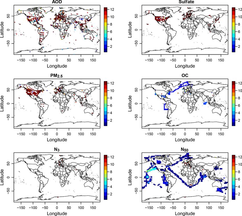
J. S. Johnson et al.: Robust observational constraint of uncertain aerosol processes                                      9493

organic aerosol (SOA) material is produced from the first-       implausible against measurements (see Sect. 2.4). The model
stage oxidation products of biogenic monoterpenes under the      variants were generated using a perturbed parameter ensem-
assumption of zero vapour pressure. SOA is combined with         ble (PPE) of 235 model simulations of HadGEM3-UKCA
primary particulate organic matter after kinetic condensation.   (the “AER PPE” detailed in Yoshioka et al., 2019) that sam-
   GLOMAP simulates new particle formation, coagulation,         ples 26 sources of uncertainty in the aerosol model (Carslaw
gas-to-particle transfer, cloud processing and deposition of     et al., 2017; Yoshioka et al., 2019); see Table A1 in Ap-
gases and aerosols. The activation of aerosols into cloud        pendix A.
droplets is calculated using globally prescribed distribu-          A set of 235 simulations alone is much too small to allow
tions of subgrid vertical velocities (West et al., 2014) and     statistical analysis of model performance across 26 dimen-
the removal of cloud droplets by autoconversion to rain is       sions of parameter space. We therefore built Gaussian pro-
calculated by the host model. Aerosols are also removed          cess emulators (surrogate models) using the PPE simulations
by impaction scavenging of falling raindrops according to        as training data (L. A. Lee et al., 2011), which define how
the parameterisation of clouds and precipitation collocation     the model outputs vary continuously over the 26-dimensional
(Boutle et al., 2014; Lebsock et al., 2013). Aerosol water       parameter space and enable dense sampling over parame-
uptake efficiency is determined by κ-Kohler theory (Petters      ter uncertainty. Separate emulators were built describing the
and Kreidenweis, 2007) using composition-dependent hy-           monthly mean value of each model output in each model grid
groscopicity factors.                                            cell. We then used Monte Carlo sampling from these emula-
   Anthropogenic emission scenarios prepared for the At-         tors to produce output for a set of 1 million model variants
mospheric Chemistry and Climate Model Intercomparison            (parameter input combinations). Uniform distributions were
Project (ACCMIP) and prescribed in some of the CMIP              assumed for each parameter in this sampling. The emulator
phase 5 experiments are used here. Biomass burning emis-         is not a perfect representation of a model output, but its un-
sions for recent decades were prescribed using a 10-year av-     certainty can be estimated and accounted for in the model–
erage of 2002 to 2011 monthly mean data from the Global          measurement comparison. In the rest of this paper, we refer
Fire and Emissions Database (GFED3; van der Werf et al.,         to the emulator-derived values of model outputs at each sam-
2010) and according to Lamarque et al. (2010) for 1850. Vol-     pled 26 d input combination as a “model variant”.
canic SO2 emissions are prescribed in the model by combin-          The AER PPE samples only uncertainties in the aerosol
ing emissions from the Andres and Kasgnoc (1998) dataset         component of the model and the radiative forcing does not
for continuously erupting and sporadically erupting volca-       account for atmospheric and cloud adjustments; i.e. it is
noes and the Halmer et al. (2002) dataset for explosive vol-     a radiative forcing (RF) rather than an effective radiative
canoes.                                                          forcing, which we analysed in previous papers (Johnson et
   A full description of the set-up for our model simulations    al., 2018; Regayre et al., 2018). The prior (unconstrained)
can be found in Yoshioka et al. (2019), which we summarise       95 % credible interval (CI) of global mean aerosol RF is
here. The base model simulation was subject to a multi-year      −2.23±0.94 W m−2 . However, because of the way that mul-
spin-up period. Parameter perturbations were then applied        tiple parameters compensate (Lee et al., 2016; Regayre et al.,
distinctly to individual ensemble members (which branch          2018), the forcing uncertainty in this PPE is similar to the
from the base model) and spun up for a further month. We         aerosol–atmosphere (AER-ATM) PPE in which additional
then ran each simulation for a further 12 months to pro-         physical atmosphere model parameters were perturbed and
duce the data used here. Horizontal winds and temperatures       cloud adjustments accounted for (Yoshioka et al., 2019). Be-
in the simulations are nudged towards European Centre for        cause the AER PPE analysed here samples only aerosol un-
Medium-Range Weather Forecasts (ECMWF) ERA-Interim               certainties, we restrict the constraints to measurements of
reanalyses for 2008 between approximately 1.2 and 80 km          aerosol properties. In future work, we will extend the anal-
using a 6 h relaxation timescale. Nudging means that pairs       ysis to radiation, precipitation and cloud measurements that
of simulations have identical synoptic-scale features, which     are relevant to the wider range of parameters in the AER-
enables the effects of perturbations to aerosol and chemical     ATM PPE.
processes to be quantified using single-year simulations, al-       The choice of the 26 perturbed parameters and their un-
though the magnitude of forcing will vary with the chosen        certainty ranges were defined using expert elicitation (Yosh-
year (Fiedler et al., 2019; Yoshioka et al., 2019).              ioka et al., 2019). The parameters (Table A1; full descriptions
                                                                 are given in Yoshioka et al., 2019) relate to natural and an-
2.2   Creation of perturbed parameter model variants             thropogenic emission fluxes of aerosol precursor gases and
                                                                 primary particles, the properties of primary particles (size),
Our method to determine observational constraint on the          aerosol processes, aerosol hygroscopicity, removal rates and
model parameters and radiative forcings involves producing       cloud droplet formation (updraft speed). The list of parame-
a very large set of “model variants”, each with a different      ters is not exhaustive, but one-at-a-time parameter perturba-
combination of parameter values, and then ruling out model       tion tests were used to show that any other parameters have
variants for which a set of model outputs are judged to be       a smaller effect regionally and globally in our model than

https://doi.org/10.5194/acp-20-9491-2020                                          Atmos. Chem. Phys., 20, 9491–9524, 2020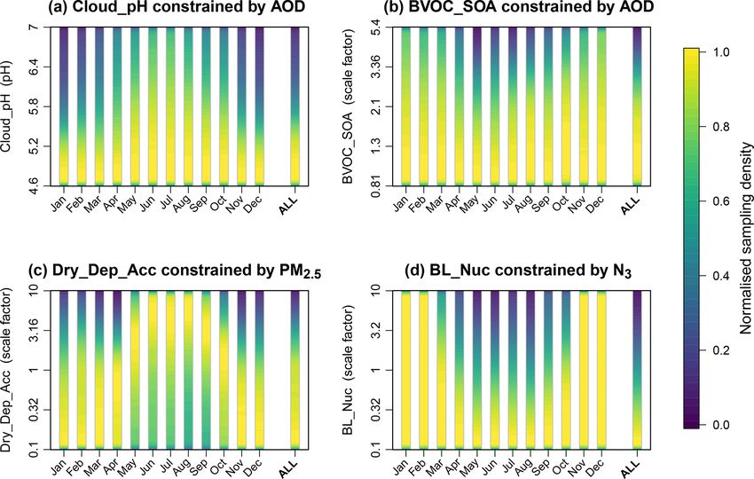
9494                                   J. S. Johnson et al.: Robust observational constraint of uncertain aerosol processes

the set we chose. Finally, we note that the evaluated uncer-     Table 1. The number of monthly aggregated grid-box measure-
tainty in global annual mean RF in this study differs from       ments for each variable in each month. The total number over all
that shown in Yoshioka et al. (2019) as we have used uni-        months and all variables is 9464.
form parameter distributions when sampling over the param-
eter uncertainty space, while elicited parameter distributions                AOD     Sulfate   PM2.5    OC     N3     N50
were used in Yoshioka et al. (2019). Our choice to use uni-           Jan      294       149      168      6     13      77
form distributions here means that the constraint can be fully        Feb      301       148      168     14     13      90
attributed to the model–measurement comparison.                       Mar      309       151      170     82     13     148
                                                                      Apr      316       151      170     74     12     199
2.3    Measurements                                                   May      322       149      167     23     12      64
                                                                      Jun      320       150      170     23     12      96
                                                                      Jul      323       148      172     23     13     115
We use aerosol measurements from ground stations, ship
                                                                      Aug      326       148      169     23     13     109
campaigns and aircraft campaigns covering the follow-
                                                                      Sep      321       147      166     22     13     133
ing aerosol properties: aerosol optical depth (AOD), PM2.5            Oct      315       147      165     41     13     119
concentrations, sulfate mass concentrations, organic carbon           Nov      309       146      168     37     13     155
mass concentrations and number concentrations of particles            Dec      298       147      169     15     12      67
larger than 3 nm dry diameter (N3 ) and 50 nm dry diame-
                                                                      Total   3754      1781     2022    383    152    1372
ter (N50 ); see Appendix B and Table S1 in the Supplement.
All measurements used are from within the boundary layer,
which we define to be at an atmospheric pressure greater than
800 hPa. We do not attempt to constrain aerosol properties       from the Interagency Monitoring of Protected Visual Envi-
above the boundary layer.                                        ronments (IMPROVE) network (USA), the European Mon-
   The measurements were all made at specific locations and      itoring and Evaluation Programme (EMEP) network and
times (i.e. they are “point measurements”) in the period from    the Acid Deposition Monitoring Network in East Asia
October 1995 to December 2015, and we use measurements           (EANET). For PM2.5 , we use data from the IMPROVE net-
from all years within this period regardless of whether the      work, the World Data Centre for Aerosols (WDCA) (Eu-
year of the measurement matches the year of the PPE model        ropean sites), the Asia-Pacific Aerosol Database (A-PAD)
simulations. (We take account of the interannual differences     and the Canadian National Air Pollution Surveillance Pro-
by incorporating an error term in the constraint process; see    gram (NAPS). Other PM2.5 measurements are included from
Sect. 2.4.) The measurements were aggregated to monthly          smaller networks and individual stations in Australia, South
mean values in grid cells of size 2.50◦ longitude by 3.75◦       America, Taiwan and South Africa, as well as sulfate and
latitude (four model grid boxes of the N96 model grid). In       PM2.5 data recorded at the Station for Observing Regional
cases where there is more than one measurement in a model        Processes of the Earth System (SORPES) in Nanjing, East
grid cell, the observed values were averaged. This processing    China. The PM2.5 data (except for the SORPES site) were
resulted in 9464 monthly aggregated grid-box measurements        obtained, processed and gridded to the N96 model grid as
(over six aerosol properties and 12 months). Figure 1 shows      described in Browse et al. (2019). Figure 1 shows that these
the global spatial coverage of the gridded measurements for      PM2.5 and sulfate measurements are highly clustered over
each aerosol property, along with the monthly temporal cov-      polluted land areas of the Northern Hemisphere, mostly in
erage for each measurement, which is indicated by the colour     North America and Europe with limited coverage elsewhere,
scale. Table 1 shows the breakdown of the number of grid-        especially in remote and marine areas. Nearly all stations in
box measurements by variable and month.                          these datasets have full temporal coverage, leading to ap-
   The AOD data are level-2.0 (quality assured) monthly          prox. 150 and 170 aggregated grid-box measurements for
mean data at 440 nm wavelength from the AERONET                  comparison in each month for PM2.5 and sulfate, respectively
(Aerosol Robotic Network) network (Giles et al., 2019; Hol-      (Table 1).
ben et al., 1998). Our dataset includes an average of 312           For N50 particle concentrations and OC concentrations,
aggregated grid-box measurements for comparison in each          we have a mixture of measurements from a small number of
month. Figure 1 shows that the measurements are well dis-        land-based ground stations along with measurements taken
tributed across all continental regions except Antarctica. The   over marine environments from ship and aircraft campaigns
coverage at high northern latitudes is relatively sparse, and    (see Appendix B and Table S1 in the Supplement). The N50
there are only a small number of island measurement that are     concentration data were mainly derived from size distribu-
representative of marine aerosol environments. The temporal      tion measurements and gridded to the N96 model grid as
coverage is very good, with the majority of stations providing   described in Browse et al. (2019). The amount of campaign
measurements in all months of the year.                          data, and hence global spatial coverage in the gridded data,
   The PM2.5 and sulfate concentration data come from            is greater for N50 than for OC (Fig. 1), and the number of ag-
multiple large networks. The sulfate concentration data are      gregated grid-box measurements is variable between months

Atmos. Chem. Phys., 20, 9491–9524, 2020                                            https://doi.org/10.5194/acp-20-9491-2020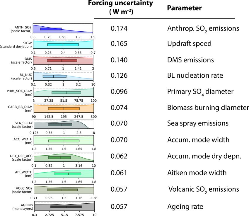
J. S. Johnson et al.: Robust observational constraint of uncertain aerosol processes                                              9495

Figure 1. The distribution of measurements used in the constraint. The colours indicate the number of months covered by the measurements
(although the data may not cover all days within a month).

(Table 1). Due to the nature of field campaigns, the temporal         2.4   Constraint methodology
coverage is much sparser for these variables, with each cam-
paign only measuring for 1–3 months of the year, shown by
                                                                      We apply the statistical methodology of history matching,
the blue colours for the data of these variables in Fig. 1.
                                                                      which has been applied to complex models in a range of
   The measurement data for N3 particle concentration have
                                                                      fields, including epidemiological modelling of virus trans-
the smallest number of grid-box measurements over the year
                                                                      mission (Andrianakis et al., 2017), risk assessment for oil
and spatially is the sparsest dataset included here. The data
                                                                      field developments (Craig et al., 1997), modelling galaxy for-
for this aerosol property come from only 13 ground stations
                                                                      mation (Rodrigues et al., 2017) and climate modelling (Ed-
(ACTRIS; Asmi et al., 2013), which are mostly located in
                                                                      wards et al., 2011; McNeall et al., 2016; Williamson et al.,
Europe, with one in the Arctic, one in Antarctica and one in
                                                                      2013). The methodology is described in detail in previous pa-
northern India. The N3 concentrations at each site were de-
                                                                      pers (Johnson et al., 2018; Regayre et al., 2018), which built
rived directly by integrating size distribution measurements.
                                                                      upon our earlier study (Lee et al., 2016). We therefore de-
These data were then averaged over multiple years for each
                                                                      scribe the overall methodology only briefly here but present
month and location by the authors.
                                                                      a full description of the new aspects related to using real mea-
                                                                      surements rather than “synthetic” measurements (Johnson et
                                                                      al., 2018).
                                                                         In the comparison of the model and measurements, we ac-
                                                                      count for emulator uncertainty, measurement uncertainty (in-

https://doi.org/10.5194/acp-20-9491-2020                                                Atmos. Chem. Phys., 20, 9491–9524, 2020
9496                                    J. S. Johnson et al.: Robust observational constraint of uncertain aerosol processes

strument error), representativeness uncertainties (caused by          The structural error term Var (S) has been included in pre-
spatial and temporal mismatches in resolution and sampling         vious studies using the implausibility metric. It is intended to
between model and measurements) and potential structural           represent an estimate of the potential structural error in the
model uncertainty. The model–measurement difference to-            model. Practically, however, we have no way to estimate this
gether with these measures of uncertainty is incorporated into     term for all variables at all times and geographical locations.
an “implausibility measure” and our model constraint proce-        We therefore set it to zero and instead use very large val-
dure in order to identify implausible parts of parameter space     ues of implausibility to point us towards potential structural
(model variants).                                                  errors in the model–observation comparison and constraint
                                                                   procedure, as described in Sect. 2.4.3.
2.4.1   Implausibility measure
                                                                   2.4.2   Estimation of uncertainty terms
The implausibility metric I (x) is calculated for each of the
1 million model variants x, for each gridded measurement.          Our estimates of the uncertainty terms in Eq. (1) are prelim-
I (x) weights the difference between the model and measure-        inary and are designed to test our approach. We discuss in
ments by the uncertainties associated with the comparison          the conclusions the need to refine our understanding of these
(Craig et al., 1996; Williamson et al., 2013)                      uncertainty terms.
                                                                      For all aerosol properties, we assume an instrument un-
                      |M − O |                                     certainty of 10 %, a spatial co-location uncertainty of 20 %
I (x) = √                                       ,            (1)
         [Var (M) + Var (O) + Var (R) + Var(S)]                    and a temporal sampling uncertainty of 10 % on the mea-
                                                                   sured value. The spatial sampling uncertainty for monthly
where M is the estimate of model output calculated using the       mean aerosol properties is estimated based on Schutgens et
emulator and O is the observed value (the measurement). In         al. (2017, 2016b). These studies examined a typical spatially
the denominator, Var (M) is the variance in the model esti-        heterogeneous continental environment where the sampling
mate (associated with replacing the model with the emula-          error is dominated mainly by local aerosol sources that are
tor), Var (O) is the variance in the measurement (i.e. instru-     not resolved by the global model. The magnitude of uncer-
ment or retrieval uncertainty), Var (R) is the variance asso-      tainty is likely to vary globally (especially between land and
ciated with the comparison of the model with the measure-          ocean), with surface measurements typically having larger
ments, called the representativeness error (Schutgens et al.,      errors than column measurements and the magnitude of error
2017, 2016a, b), and Var (S) is a model structural error term.     also depending on the location of a ground site with respect
    A low value of the implausibility metric indicates either      to the grid-box centre, but we do not account for these varia-
the model–measurement difference is small (i.e. the model is       tions. We base our estimate of the temporal sampling uncer-
skilful) or that the uncertainty in the denominator is large       tainty on Schutgens et al. (2016a), who quantified the error
(i.e. we cannot tell whether the model is skilful because          associated with the different temporal sampling of models
the uncertainties are too large). Therefore, the implausibility    and measurements (daily measurements or temporally spo-
metric allows model variants to be ruled out if the model–         radic measurements versus monthly mean model, etc.). The
measurement difference is large and we can be confident that       emulator uncertainty is taken from the Gaussian error on the
it is large.                                                       emulator mean prediction, which is known for every param-
    The representativeness
                             error Var (R) has three compo-       eter combination (i.e. each of the 1 million model variants).
nents. Var Rsp (sp: spatial) accounts for uncertainty associ-         The interannual uncertainty was defined to be the standard
ated with spatial variability below the grid scale of the model,   deviation of monthly mean aerosol properties in each grid
which means that a point measurement may not be repre-             cell over a 30-year period. We take information from an anal-
sentative of  the grid-box mean (Schutgens et al., 2016b).        ysis of the trend and variation of gridded aerosol properties
Var Rtemp (temp: temporal) accounts for the temporal sam-          in a HadGEM3-UKCA hindcast simulation over the period
pling of a measurement, which may not match the temporal           of 1980–2009 (Turnock et al., 2015). For each month and
sampling of the model (e.g. a ship track through the grid box      grid box, the monthly mean output of the aerosol variable of
over a short time period which is compared with a monthly          interest for each year of the simulation was obtained. These
mean model value (Schutgens et al., 2016a). Var (Riav ) (iav:      values were de-trended using linear regression and the result-
interannual variability) accounts for the fact that we some-       ing residuals were then analysed. We use a relative measure
times match measurements and the model for the correct cal-        of monthly mean uncertainty defined by the standard devia-
endar month but not for the correct year. This is necessary in     tion of these residuals divided by the de-trended mean. As an
cases where we use measurements from years for which we            example, Fig. 2 shows the relative standard deviation for the
have not run the model. We assume that                             surface-level N50 concentration in July.

Var (R) = Var Rsp + Var Rtemp + Var (Riav ) .                (2)

The magnitude of these errors is discussed in Sect. 2.4.2.

Atmos. Chem. Phys., 20, 9491–9524, 2020                                              https://doi.org/10.5194/acp-20-9491-2020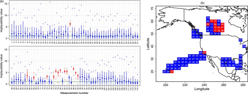
J. S. Johnson et al.: Robust observational constraint of uncertain aerosol processes 9497
in a particular month. Figure 4 shows an example for
the measurements of N50 in July. For each measurement
(numbered on the horizontal axis in Fig. 4a), the distri-
bution of the implausibility over the variants is shown
by the bar representing the 95 % credible interval.
2. Measurements are identified for which 97.5 % of the
model variants have an implausibility I > 1. These
measurements are excluded from the constraint proce-
dure (shown in red in Fig. 4). We assume that this large
implausibility for the significant majority of variants in-
dicates that either there is a structural error in the model
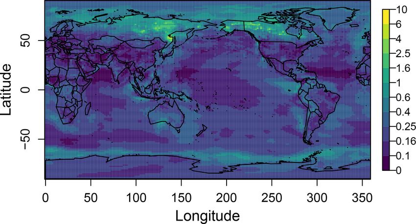
Figure 2. The relative standard deviation for surface-level N50 con- or that the model is unable to represent these point mea-
centration in July, used in the estimation of the interannual variabil- surements because of its low spatial and temporal reso-
ity component of representativeness error Riav . lution. An alternative explanation is a mismatch in the
model’s meteorological year to the year of the measure-
ment (Sect. 2.4.1). We flag these measurements for fur-
2.4.3 Methodology for ruling out observationally ther investigation of potential structural errors or under-
implausible parts of parameter space estimated error terms (these are not examined further in
this study).
There is an element of subjectivity involved in comparing a
model with point measurements and reaching a conclusion 3. Using all other measurements (where more model
about the fidelity of the model. The comparison may indicate variants have lower implausibility, shown in blue in
either (a) the model seems to be structurally adequate, but Fig. 4), we use the implausibility metric values to de-
the parameters need to be adjusted to optimise agreement, cide whether to rule each variant out as implausible or
or (b) the model is structurally deficient (i.e. there are miss- retain it as plausible. If we ruled out all model variants
ing or incorrect process representations in the model). Struc- with high implausibility for each measurement in turn
tural deficiencies may be apparent, for example, because the (treating the measurements independently, as in many
model skill is particularly poor in one region or at one time of emergent constraint studies), we could end up ruling out
year, or it is not possible to obtain good skill across multiple all parts of parameter space. Our criterion is therefore to
variables simultaneously. rule out a model variant if more than a defined fraction
Our use of 1 million model variants and more than 9000 (or number) of the measurements (tolerance T ) exceeds
monthly aggregated grid-box measurements means that we a defined implausibility threshold (θ). For example, we
need to automate the model–measurement comparison pro- might rule out a model variant if more than 20 % of mea-
cesses and detection of potential structural errors while also surements exceed an implausibility of 3.5 (i.e. bias is
using the measurements to rule out implausible parts of pa- 3.5 times the expected error).
rameter space. The difficulties for us in detecting structural
errors are as follows: (a) we cannot inspect each of the 1 mil- We apply this approach to the set of measurements for each
lion model variants individually, so we need to rely on sum- variable (measurement type) in each month and then com-
mary statistics; (b) many of the aerosol point measurements bine the constraints to a joint constraint over months and/or
are spatially and temporally sparse, so we cannot easily de- over variables such that if a variant is ruled out for any sin-
tect spatial and temporal changes in model skill that might in- gle month/variable combination, then it is also ruled out in
dicate structural error; (c) the measurements do not have the the joint constraint. This method allows us to identify the set
same spatial distribution in all months (because of brief, lo- of model variants that capably represent measurements of a
calised field campaigns) so spatial–temporal biases are hard range of variables and across multiple locations and seasons.
to detect; (d) the uncertainty in each measurement (particu- We extensively explored various choices of the tolerance and
larly the representativeness error, Sect. 2.4.2) is spatially and threshold values in each variable/month case and found that
temporally heterogeneous and often very poorly defined. the final constrained parameter ranges were reasonably ro-
Our approach is summarised in Fig. 3. It is designed to bust, except when the number of measurements was small.
rule out implausible parts of parameter space while avoiding Our choices of the threshold and tolerance for each mea-
doing so in cases where the biases shared by many model surement type are given in Table A2 in Appendix A. A wide
variants could be caused by structural errors in the model. range of values were tested in each case, starting with a set
The steps are as follows: threshold of θ = 3.5 and iterating through increasing toler-
ances T up to a maximum of T = 33 % (1/3 of the measure-
1. The implausibility is quantified for each of the 1 mil- ments), before further increasing θ by 0.5 (to a maximum of
lion variants across all measurements of a single type θ = 4.5) and re-iterating over T in order to retain (approx-
https://doi.org/10.5194/acp-20-9491-2020 Atmos. Chem. Phys., 20, 9491–9524, 2020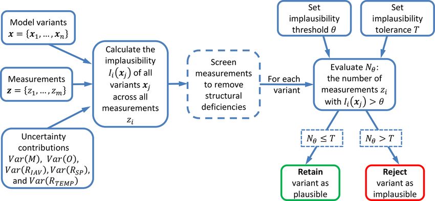
9498                                       J. S. Johnson et al.: Robust observational constraint of uncertain aerosol processes

Figure 3. Flowchart detailing the process followed for each model variant x j , in using the calculated implausibility over a set of m measure-
ments z = {z1 , z2 , · · ·, zm } (for a single output variable y) simultaneously to constrain the model uncertainty.

Figure 4. (a) The distribution of implausibility calculated over the 1 million model variants for each measurement in the July N50 concen-
tration set, shown vertically. For each measurement, numbered along the x axis, the range of the implausibility distribution is shown by the
outer crosses, the bar corresponds to the 95 % credible interval (2.5 % to 97.5 % empirical quantiles), the horizontal markers through the bar
show the interquartile range, and the square point is the median implausibility. Here, we assume no structural error term in the implausibility
calculations and use the implausibility distribution to identify potential structural errors. Measurements coloured red are ruled out as poten-
tial structural error cases (as the lower 95 % credible interval bound is > 1), and those coloured blue are retained and used in our constraint
procedure. (b) Corresponding map to show the locations of the rejected July N50 measurements (red) and those retained for constraint (blue),
over the North Pacific and North American region (outside this region, all measurements were retained). We hypothesise that the red points
over the Pacific correspond to ports with localised pollution sources, while the red points over Canada correspond to localised fire emissions
that are not represented at the resolution of the model.

imately) a chosen percentage of model variants. Approxi-                  able number of model variants and avoid overconstraining on
mately the same percentage of variants was attained for all               any one observational type.
months of a variable type and combined for an “all-months”                   Our assumption of zero structural error (Var (S) = 0) in
constraint. Our final choices for each variable type on its own           the implausibility calculations means that structural errors
(left column in Table A2) were relaxed for the joint “all-                in the model can easily come to light in our constraint pro-
variables-months” constraint (retaining a larger percentage               cess. This occurs either in the calculated implausibility val-
of variants in each month for each variable, so a weaker con-             ues for a measurement (where large values are consistently
straint; right column in Table A2), in order to retain a reason-          produced over the 1 million variants covering the model
                                                                          uncertainty, indicating a large model–measurement discrep-

Atmos. Chem. Phys., 20, 9491–9524, 2020                                                      https://doi.org/10.5194/acp-20-9491-2020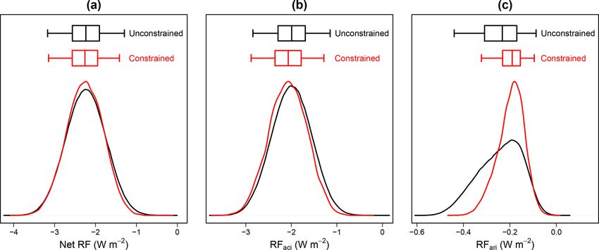
J. S. Johnson et al.: Robust observational constraint of uncertain aerosol processes 9499
ancy, e.g. Fig. 4) or when bringing together the constraint rate constrained parameter PDFs do not overlap can we con-
effects of different sets/types of measurements (where very clude with certainty that there is likely to be a structural de-
few, if any, model variants that lead to plausible model out- ficiency in the model. However, to obtain multivariate con-
put in all cases/measurement types simultaneously can be straint, we prevent this happening by screening out measure-
identified and retained). Even though we do not directly ac- ments with large model–measurement discrepancies and re-
count for structural errors in the implausibility measure it- laxing the constraint criteria with each measurement type.
self, our constraint approach offsets the effects of such er-
rors on the achieved constraint as much as possible. This
is accomplished by screening out observations with large 3 Results
model–measurement discrepancies from the constraint pro-
cess (step 2; Fig. 4) and by relaxing the constraint criteria 3.1 Constraint using individual measurement types
for the joint all-variables-months constraint. Through this ap-
proach, we are able to produce as robust a constraint as pos- Figure 6 shows the constrained marginal parameter distribu-
sible, given the limitations we have in specifying structural tions for all parameters based on using individual measure-
and representational errors. ment types (each column on left) and all measurement types
together (right column).
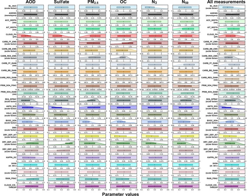
2.5 Interpretation of constrained parameter AOD measurements constrain aerosol and precursor emis-
probability distributions sions to low values and removal rates to high values. These
constraints imply that the PPE produces generally too-high
Observationally plausible parts of parameter space ex- AODs across the sampled parameter space, which is the
ist in 26 dimensions. We show the results as one- case (Sect. 3.4). In particular, sea spray emissions higher
dimensional marginal probability distributions, which are than about 3.6 times the baseline emissions are ruled out,
one-dimensional projections of the 26-dimensional param- but emissions down to as low as 0.125 times the base-
eter probability distribution. Figure 5 shows an idealised rep- line emissions are plausible. For anthropogenic SO2 emis-
resentation for a two-dimensional parameter constraint. The sions, the likelihood of the emissions scale factor being be-
white parts of the joint distribution are ruled out, leaving low 1 (corresponding to the default value from the inven-
the shaded region of joint parameter space as observation- tory) increases from 55 % to 70 % on constraint. For biogenic
ally plausible. The effect on the marginal probability distri- volatile organic compound (BVOC) emissions, the likelihood
bution of parameter 1 is to entirely rule out the lowest and of the emissions (or effectively the production of SOA) be-
highest values (i.e. there is no combination of these values ing more than 3 times the default emission of 46 Tg yr−1
of parameter 1 with parameter 2 that produces an observa- (= 138 Tg yr−1 ) is reduced from 31 % to 13 %, but all lower
tionally plausible model). Where some values of parameter 1 values from the default emission down to our lower bound of
are ruled out over the range of parameter 2, the likelihood of 37 Tg yr−1 are equally plausible.
parameter 1 having those values is reduced. The AOD measurements also constrain the model to low
In the results below, the parameter probability distribu- values of other parameters: more variants with higher cloud
tions therefore reflect the relative likelihood of the parameter droplet pH values are ruled out (judged implausible) and as
having particular values, with lower probabilities indicating a result cloud droplet pH is nearly 3 times as likely to be be-
that there are fewer ways in which the parameter can be com- low the central value of its range of 5.8 as above it, which
bined with the other 25 parameters to produce a plausible is consistent with a higher likelihood of slower production
model. For conciseness in the results section, we say, for ex- of sulfate aerosol from in-cloud SO2 oxidation. The hygro-
ample, that “a measurement constrains the parameter to low scopicity of OC in the particles (κOC ) is also weakly con-
values”, which means that we retain a larger proportion of strained to low values, which reduces the water content of
model variants with low values. aerosol and reduces AOD. The rate of aerosol scavenging by
Figure 5 also shows the separate and joint effects of two precipitating raindrops (the Rain_Frac parameter) is weakly
observational constraints. We show this conceptually be- constrained to high values.
cause it arises in the results. Measurement 1 rules out the Sulfate measurements strongly constrain SO2 emissions
lowest values of parameter 1 and suggests that parameter 1 to low values, which is consistent with the AOD constraint.
is likely to be at the high end of the sampled range. Con- Given this constraint, the SO2 emissions have a 78 % like-
versely, measurement 2 suggests that parameter 1 is likely to lihood of being below the default value from the inventory
be at the low end of the range. However, the correct inter- and the median emission is reduced to 0.78 times the default.
pretation of this situation is that intermediate values of the Also consistent with the AOD constraint, the deposition rate
parameter are consistent with both measurements (measure- of accumulation-mode particles is constrained strongly to
ment 1 is consistent with the model for all but the lowest high values, with an 87 % likelihood of the rate being above
values of the parameter and measurement 2 is consistent for the default value. Likewise, the SO2 dry deposition rate is
all but the highest values). Only in cases where the two sepa- constrained fairly weakly to higher values, with a 60 % likeli-
https://doi.org/10.5194/acp-20-9491-2020 Atmos. Chem. Phys., 20, 9491–9524, 20209500 J. S. Johnson et al.: Robust observational constraint of uncertain aerosol processes Figure 5. Schematic of parameter constraint in two dimensions using two measurements. hood of the scaled value being above the default value. Each way to PM2.5 and AOD, with scaled emissions above about of these constraints is consistent with too-high sulfate con- a factor of 2.1 (97 Tg yr−1 ) having only a 31 % likelihood centrations in many of the sampled model variants across the (compared to 50 % prior to constraint). OC measurements parameter uncertainty space (Sect. 3.4). also constrain the lowest values of BVOC emissions, which PM2.5 measurements have a similar effect to AOD on some was not achieved with PM2.5 and AOD. The likelihood of the parameters, but for others there are differences. Emissions scaled emissions being below 1 (46 Tg yr−1 ) is 6 % (com- of sea spray and BVOC emissions are constrained similarly pared with 11 %). The dry deposition rate of Aitken-mode (to low values). However, SO2 emissions and cloud droplet particles is constrained to the low part of the range, which pH are weakly constrained to higher values and the dry de- will tend to increase OC concentrations in the atmosphere position rate of accumulation-mode particles is weakly con- consistent with the constraint of fossil fuel emissions to high strained to low values, opposite to the AOD and sulfate con- values. There is also a weak constraint of the ageing rate to- straints for these parameters. The PM2.5 measurements also wards higher values, which has a 55 % likelihood of being weakly constrain the residential combustion emissions to in the upper half of the range. The rate of aerosol scaveng- high values. PM2.5 and AOD are strongly correlated in the ing by precipitating raindrops (Rain_Frac parameter) is con- PPE (Johnson et al., 2018), so differences in the constrained strained similarly but to lower values. Again, although weak, parameters most likely reflect differences in the spatial distri- these two constraints imply slower ageing, slower removal bution of the measurements (Fig. 1) and how that maps onto rates, longer OC lifetime and higher atmospheric concentra- the spatial variations in sensitive parameters. As described in tions. Biomass burning emissions are only very weakly con- Sect. 2.5, these apparently opposing constraints are not nec- strained towards lower emissions. The lack of constraint on essarily inconsistent: for AOD and PM2.5 , there may be other the biomass burning emissions from OC measurements here parameter settings that can be combined with low SO2 emis- is likely a result of the limited coverage, if any, of the OC sions to achieve agreement with the measurements (so the measurements in regions important for biomass burning such space is not ruled out). as Africa and southeast Asia (Fig. 1). OC measurements strongly constrain the scaled magnitude Particle concentration (N3 and N50 ) measurements con- of residential carbonaceous emissions to a narrower credi- strain a wider range of parameters than the measurements ble interval of about 0.3–1.8 centred near the default value of mass-related properties. The rate of boundary layer nu- specified in the emissions. Emissions above 2.0 times the cleation is strongly constrained to the low part of the sam- default value are effectively ruled out and there is only a pled range by the N3 measurements (a 77 % likelihood of be- 13 % likelihood of the emissions being below half the de- ing below the default rate), suggesting N3 concentrations are fault value. Fossil fuel emissions have a 70 % likelihood of generally too high across the PPE. N3 also weakly constrains being above the default emission value. The OC measure- the dry deposition of Aitken- and accumulation-mode parti- ments also constrain the scaled BVOC emissions in a similar cles to low values. Low deposition rates of accumulation- Atmos. Chem. Phys., 20, 9491–9524, 2020 https://doi.org/10.5194/acp-20-9491-2020
J. S. Johnson et al.: Robust observational constraint of uncertain aerosol processes                                                     9501

Figure 6. Marginal parameter distributions after constraint using individual measurement types over all months (six columns on the left) and
after using all measurement types over all months together (right column). The 25th, 50th and 75th percentiles of each constrained distribution
are shown in the central boxes, and the parameter values on the x axes correspond to values as they are used in the model (parameters that are
multiplicative scaling factors are shown on the log10 scale), covering the full parameter ranges (Yoshioka et al., 2019). The corresponding
choices of threshold θ and tolerance T that were applied in the constraint process to generate these results are given in Table A2 (left column
for each individual measurement type; right column for the joint measurement-type constraint), along with the percentage of model variants
that is retained in the constrained sample in each case. See Sect. 2.5 for a definition of marginal parameter distributions.

mode particles (hence higher atmospheric concentrations)                  constrained by N3 measurements, even though SOA enters
will result in a higher condensation sink and more removal                the nucleation rate expression. This is most likely because
of sulfuric acid that participates in particle nucleation, so             high BVOC emissions also enhance total SOA, which acts as
this is consistent with the constraint of nucleation rates to             a condensation sink for nucleation, so the two effects cancel
low values. The constraint of Aitken-mode deposition to low               (Carslaw et al., 2013b).
values is less obvious. Aitken-mode particles can contribute                 For N50 , the constraints are consistent with shifting the
substantially to N3 , so low deposition rates would enhance               N50 concentrations in the ensemble towards lower values
N3 (opposite to the constraint on nucleation rates). However,             (Sect. 3.4). N50 has very little effect on the range of bound-
nucleation rates are constrained to very low values, so in such           ary layer nucleation rate. In contrast, a previous study found
a situation Aitken particles can begin to act as a sink term for          that boundary layer nucleation made a statistically signifi-
nucleation by affecting the condensation sink and by growing              cant difference to model skill at about half of the ground
into accumulation-mode particles. BVOC emissions are not                  sites they analysed (Reddington et al., 2011) – although that

https://doi.org/10.5194/acp-20-9491-2020                                                    Atmos. Chem. Phys., 20, 9491–9524, 2020
9502                                     J. S. Johnson et al.: Robust observational constraint of uncertain aerosol processes

study tested the effect of including or not including bound-        are high. Microphysical process rates (dry deposition of ac-
ary layer nucleation rather than perturbing the rate as we do       cumulation mode and wet scavenging rates) are consistently
here. Without boundary layer particle formation, the model          constrained throughout the year.
was structurally deficient and had poor skill at around half the       For PM2.5 , the seasonality of constraint is very similar to
sites analysed. However, our results show that uncertainty in       AOD with one notable exception. The dry deposition rate of
the parameter value itself is unimportant when other param-         accumulation-mode particles is constrained to high values in
eter uncertainties are considered. This parameter is uncon-         summer (consistent with AOD and sulfate) but to low values
strained by N50 measurements because there are many alter-          in the winter (Fig. 7c). This may occur just because of the
native ways of achieving model–measurement agreement.               way in which the combinations of parameters control PM2.5 ;
   N50 measurements also tend to constrain primary parti-           for example, BVOCs can account for PM2.5 in summer so
cle emissions to the lower end of the range (fossil fuel and        high dry deposition rates cannot be ruled out. However, it
primary sulfate emissions), albeit weakly. Residential parti-       may also indicate a structural deficiency. The low deposi-
cle emissions are not constrained, but the measurements we          tion rates in winter imply that PM2.5 has missing sources
used are not well located to achieve this. It also constrains the   in winter but not in the summer, such as nitrate. Our model
emitted particle diameters to the high end of their ranges (fos-    does not include aerosol nitrate, which (if included) would
sil fuel, primary sulfate), which is again consistent with low      increase Northern Hemisphere winter PM2.5 concentrations
number concentrations (since we perturb emission diameter           and weaken the constraint on dry deposition towards lower
independently of the mass, so number concentration is af-           values in Northern Hemisphere winter.
fected). The constraint of particle emission sizes is consistent       For N3 , we find that the boundary layer nucleation rate is
with a previous study that showed cloud condensation nu-            constrained only in summer when photochemical production
clei (CCN) concentrations are sensitive to the assumed size         of the nucleating vapours is fast (Fig. 7d). This is consistent
(Reddington et al., 2011). Our results show that N50 mea-           with previous studies that have examined the seasonal cy-
surements allow the emission size to be constrained, even           cle of organic-mediated nucleation (Riccobono et al., 2014).
though there are many other compensating factors that can           Similarly, N3 measurements constrain SO2 emissions and
affect CCN concentrations. N50 weakly constrains cloud pH           cloud droplet pH in summer when nucleation is most active.
to higher values, consistent with greater production of sul-        This is in contrast to the AOD and sulfate measurements,
fate aerosol and a higher sink for nucleation. BVOC emis-           which constrained these two parameters in winter when their
sions are constrained to the low end, which is consistent           relative contribution to aerosol mass is greater.
with reduced growth of nucleation-mode particles into the              For N50 , we find that parameter constraints do not vary
Aitken and accumulation modes. N50 also constrains deposi-          smoothly throughout the year (not shown). This is because
tions rates: accumulation-mode deposition is constrained to         the N50 measurements we have used are primarily from cam-
low values and Aitken-mode deposition to high values, sug-          paigns, which move around the globe, resulting in constraint
gesting a shift in the aerosol size distribution towards larger     of regionally important parameters. This is one indication
aerosols is consistent with N50 measurements.                       that we need to add long-term network measurements of N50
                                                                    to the dataset.
3.2    Seasonal variations in constraint
                                                                    3.3   Constraint using all measurement types
Many of the parameter constraints vary seasonally, which can
be linked to seasonal variations in emissions and parameter
sensitivity. Some examples are shown in Fig. 7. Cloud pH            The multivariate constraint is shown as the right-hand col-
is constrained more by AOD in Northern Hemisphere win-              umn of PDFs in Fig. 6 and Table 2 shows corresponding pa-
ter (Fig. 7a) when in-cloud oxidation of SO2 by ozone dom-          rameter distribution statistics from this constraint. For each
inates sulfate production. BVOCs are constrained by AOD             individual variable/month constraint that feeds into this mul-
only in Northern Hemisphere summer when the emissions               tivariate constraint, the implausibility threshold and toler-
are strong (Fig. 7b). There are several other seasonal varia-       ance criteria (θ and T ) were relaxed from the individual
tions in the constraint effect from AOD measurements that           measurement constraints to retain approximately 75 % of the
we do not show. For example, anthropogenic SO2 emissions            1 million model variants (Table A2). This relaxed criterion
are constrained by AOD more in winter because the AOD               leads to measurements that provide stronger constraint being
uncertainty in summer is dominated by the uncertainty in            downweighted and individual parameter constraints becom-
SOA. The hygroscopicity of OC is also constrained more              ing weaker, but it means that we are able to avoid overcon-
in summer when OC is a larger component of the aerosol.             straining on any one measurement type. Using all measure-
Biomass burning emissions are constrained in NH summer as           ment types together leads to retention of only 2.1 % of the
expected from wildfire emission seasonality and the North-          original 1 million model variants as plausible models (nearly
ern Hemisphere bias of our measurements dataset. Residen-           98 % rejected; Table A2). In most cases, the marginal param-
tial emissions are only constrained in winter when emissions        eter distributions from this constraint can be understood in

Atmos. Chem. Phys., 20, 9491–9524, 2020                                              https://doi.org/10.5194/acp-20-9491-2020
J. S. Johnson et al.: Robust observational constraint of uncertain aerosol processes 9503 Figure 7. Seasonal variation in the constraint of parameter marginal probability distributions. The examples are (a) constraint of the pH of cloud droplets (Cloud_pH) parameter using global AOD measurements, (b) constraint of SOA production from BVOCs (BVOC_SOA) using AOD measurements, (c) constraint of the dry deposition rate of accumulation-mode particles (Dry_Dep_Acc) using global PM2.5 measurements and (d) constraint of boundary layer nucleation rates (BL_Nuc) using N3 measurements mainly over Europe. terms of the combination of individual constraints described ues below this down to 0.25 times the default value are still above. equally likely, as they were before constraint. Boundary layer nucleation rates are constrained to the low Residential carbonaceous emissions are constrained pri- end of the range, which can be attributed almost entirely marily through a combination of PM2.5 and OC measure- to the N3 measurements. However, the constraint is slightly ments. This emissions scaling parameter is constrained to weaker than when just N3 measurements are used because of be most likely near the middle of its range around the de- the need to relax the tolerances and thresholds applied when fault setting, with emissions higher than about 2.7 times the ruling out model variants using multiple measurement types default emission rate ruled out completely and also some (Sect. 2.4.3). The nucleation rate is constrained such that the weaker constraint at the lower end of the range. The 95 % likelihood of it being in the lower half of the range (0.1–1 credible interval has significantly shifted towards lower val- times the default value) is 70 % – more than twice the like- ues, from 0.27–3.73 times the default value before constraint lihood of it being in the upper half of the range (1–10 times to 0.27–1.85 times the default value after constraint, with the the default value). constrained interquartile range being 0.46–1.06 (Table 2). The pH of cloud droplets, which controls aqueous-phase The diameter of fossil fuel particles is constrained mainly oxidation of SO2 to form sulfate aerosol, is constrained to through the N50 measurements towards larger diameters, be more likely in the middle of our elicited range. This re- with a likelihood of being in the upper half of our elicited sults from a combination of AOD and sulfate measurements range (60–90 nm diameter) of 61 % and the median of this constraining it to the lower end of the range and PM2.5 mea- parameter distribution shifting to a larger diameter on con- surements constraining it to the higher end. Observational straint, increasing from 60 to 65.63 nm. constraint is unable to rule out any of the pH values between Sea spray emissions are constrained through a combina- 4.6 and 7.0, although there is a reduction of 0.13 in the 95 % tion of AOD and PM2.5 measurements, and to a lesser extent credible interval to 4.69–6.84 (from 4.66–6.94 before con- by N50 . The multivariate constraint is slightly weaker than straint) and a larger reduction of 0.32 in the interquartile was achieved by AOD and PM2.5 individually, although we range to 5.24–6.12 (from 5.2–6.4 before constraint). are still able to rule out emissions in the range 4.7–8 times Biomass burning emissions are weakly constrained. The the default value. Emissions in the range 0.125–2.8 times the likelihood of emissions being more than a factor of 2 above default value are not strongly constrained by any of the mea- the default value is reduced to 14 % (from 25 %), but all val- surements. https://doi.org/10.5194/acp-20-9491-2020 Atmos. Chem. Phys., 20, 9491–9524, 2020
You can also read