Quantifying new water fractions and transit time distributions using ensemble hydrograph separation: theory and benchmark tests - HESS
←
→
Page content transcription
If your browser does not render page correctly, please read the page content below
Hydrol. Earth Syst. Sci., 23, 303–349, 2019
https://doi.org/10.5194/hess-23-303-2019
© Author(s) 2019. This work is distributed under
the Creative Commons Attribution 4.0 License.

Quantifying new water fractions and transit time distributions using
ensemble hydrograph separation: theory and benchmark tests
James W. Kirchner1,2,3
1 Dept. of Environmental Systems Science, ETH Zurich, 8092 Zurich, Switzerland
2 Swiss Federal Research Institute WSL, 8903 Birmensdorf, Switzerland
3 Dept. of Earth and Planetary Science, University of California, Berkeley, CA 94720, USA

Correspondence: James W. Kirchner (kirchner@ethz.ch)

Received: 9 August 2018 – Discussion started: 27 August 2018
Revised: 4 December 2018 – Accepted: 12 December 2018 – Published: 18 January 2019

Abstract. Decades of hydrograph separation studies have           the shapes of the transit time distributions, nor does it as-
estimated the proportions of recent precipitation in stream-      sume that they are time-invariant, and it does not require
flow using end-member mixing of chemical or isotopic trac-        continuous time series of tracer measurements. Benchmark
ers. Here I propose an ensemble approach to hydrograph            tests with a nonlinear, nonstationary catchment model con-
separation that uses regressions between tracer fluctuations      firm that ensemble hydrograph separation reliably quantifies
in precipitation and discharge to estimate the average frac-      both new water fractions and transit time distributions across
tion of new water (e.g., same-day or same-week precipita-         widely varying catchment behaviors, using either daily or
tion) in streamflow across an ensemble of time steps. The         weekly tracer concentrations as input. Numerical experi-
points comprising this ensemble can be selected to isolate        ments with the benchmark model also illustrate how ensem-
conditions of particular interest, making it possible to study    ble hydrograph separation can be used to quantify the effects
how the new water fraction varies as a function of catch-         of rainfall intensity, flow regime, and antecedent wetness on
ment and storm characteristics. Even when new water frac-         new water fractions and transit time distributions.
tions are highly variable over time, one can show mathemat-
ically (and confirm with benchmark tests) that ensemble hy-
drograph separation will accurately estimate their average.
Because ensemble hydrograph separation is based on corre-         1   Introduction
lations between tracer fluctuations rather than on tracer mass
balances, it does not require that the end-member signatures      For nearly 50 years, chemical and isotopic tracers have been
are constant over time, or that all the end-members are sam-      used to quantify the relative contributions of different water
pled or even known, and it is relatively unaffected by evapo-     sources to streamflow following precipitation events (Pinder
rative isotopic fractionation.                                    and Jones, 1969; Hubert et al., 1969); see also reviews by
   Ensemble hydrograph separation can also be extended            Buttle (1994) and Klaus and McDonnell (2013), and refer-
to a multiple regression that estimates the average (or           ences therein. As reviewed by Klaus and McDonnell (2013),
“marginal”) transit time distribution (TTD) directly from ob-     chemical and isotopic hydrograph separation studies have
servational data. This approach can estimate both “back-          led to many important insights into runoff generation. Fore-
ward” transit time distributions (the fraction of streamflow      most among these has been the realization that even at storm-
that originated as rainfall at different lag times) and “for-     flow peaks, stream discharge is often composed primarily of
ward” transit time distributions (the fraction of rainfall that   “old” catchment storage rather than “new” recent precipi-
will become future streamflow at different lag times), with       tation (Sklash et al., 1976; Sklash, 1990; Neal and Rosier,
and without volume-weighting, up to a user-determined max-        1990; Buttle, 1994). The previous dominant paradigm, based
imum time lag. The approach makes no assumption about             on little more than intuition, had held that because stream-
                                                                  flow responds promptly to rainfall, the storm hydrograph

Published by Copernicus Publications on behalf of the European Geosciences Union.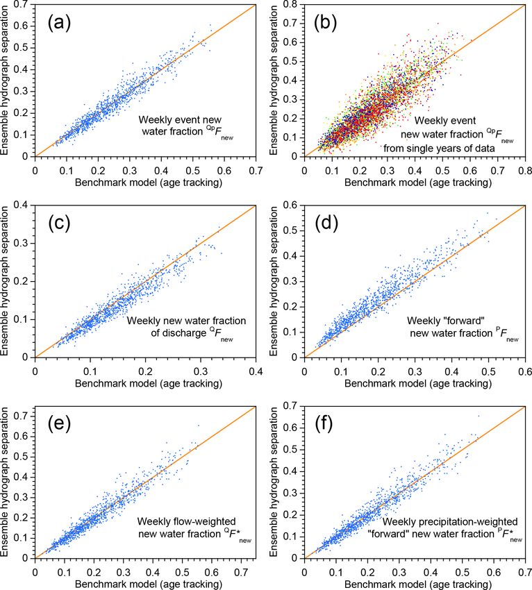
304                                                                      J. W. Kirchner: Ensemble hydrograph separation

must consist primarily of precipitation that reaches the chan-     1. Hydrograph separation studies often lead to implausible
nel quickly. Isotope hydrograph separations showed that               (including negative) inferred contributions of new wa-
this intuition is often wrong, because the isotopic signa-            ter, and such anomalous results are sometimes attributed
tures of stormflow often resemble baseflow or groundwater             to contributions from un-sampled end-members (e.g.,
rather than recent precipitation. These observations have not         von Freyberg et al., 2017). In such cases, assumption
only overthrown the previous dominant paradigm, but also              no. 1 is clearly not met.
launched decades of research aimed at unraveling the para-
dox of how catchments store water for weeks or months,             2. The isotopic composition of precipitation can vary con-
but release it within minutes following the onset of rainfall         siderably within an event, both spatially and temporally,
(Kirchner, 2003).                                                     even in small catchments (e.g., McDonnell et al., 1990;
   The foundations of conventional two-component hydro-               McGuire et al., 2005; Fischer et al., 2017; von Frey-
graph separation are straightforward. If one assumes that             berg et al., 2017). Likewise, the isotopic signature of the
streamflow is a mixture of two end-members of fixed compo-            baseflow or groundwater end-member has been shown
sition, which I will call for simplicity “new” and “old” water,       to vary in space and time during snowmelt and rain-
then at any time j the mass balance for the water itself is           fall events (e.g., Hooper and Shoemaker, 1986; Rodhe,
                                                                      1987; Bishop, 1991; McDonnell et al., 1991). In these
Qj = Qnewj + Qoldj ,                                       (1)        cases, assumptions no. 2 and 3 are not met. Various
                                                                      schemes have been proposed to address this spatial and
and the mass balance for a conservative tracer is                     temporal variability by weighting the isotopic compo-
                                                                      sitions of individual samples, but the validity of these
                                                                      schemes typically rests on strong assumptions about the
Qj CQj = Qnewj Cnew + Qoldj Cold ,                         (2)        nature of the runoff generation process and the hetero-
                                                                      geneity to be averaged over.
where Q denotes water flux and C denotes the concentration
of a passive chemical tracer or the δ value of 18 O or 2 H. One    3. When the difference between Cnew and Cold is not large
can straightforwardly solve Eqs. (1) and (2) to express the           compared to their uncertainties, Eq. (3) becomes un-
fraction of new water in streamflow at any time j as                  stable and the resulting hydrograph separations become
                                                                      unreliable. This problem can be detected using Gaus-
          Qnewj       CQj − Cold
Fnewj =           =                 .                      (3)        sian error propagation (Genereux, 1998), but Bansah
           Qj         Cnew − Cold                                     and Ali (2017) report that less than 20 % of the hydro-
                                                                      graph separation studies they reviewed have used it.
   In typical applications, the new water is recent precipita-
tion and the tracer signature of the old water is obtained from   One can agree with Buttle (1994) that “despite frequent vi-
pre-event baseflow, which is generally assumed to originate       olations of some of its underlying assumptions, the isotopic
from long-term groundwater storage.                               hydrograph separation approach has proven to be sufficiently
   The assumptions underlying conventional hydrograph sep-        robust to be applied to the study of runoff generation in
aration can be summarized as follows:                             an increasing number of basins,” at least as a characteriza-
 1. Streamflow is a mixture formed entirely from the sam-         tion of the community’s widespread acceptance of the tech-
    pled end-members; contributions from other possible           nique. Nonetheless, there is clearly room for new and dif-
    streamflow sources (such as vadose zone water or sur-         ferent ways to quantify stormflow generation. In addition,
    face storage) are negligible.                                 weekly or even daily isotope measurements are now becom-
                                                                  ing available for many catchments, sometimes spanning peri-
 2. The samples of the end-members are representative             ods of many years, and despite their many uses (particularly
    (e.g., the sampled precipitation accurately reflects all      for calibrating hydrological models) there is an obvious need
    precipitation, and the sampled baseflow reflects all pre-     for new ways to extract hydrological insights from such time
    event water).                                                 series.
                                                                     Here I propose a new method for using isotopes and other
 3. The tracer signatures of the end-members are constant         conservative tracers to quantify the origins of streamflow.
    through time, or their variations can be taken into ac-       This method is based on statistical correlations among tracer
    count.                                                        fluctuations in streamflow and one or more candidate water
 4. The tracer signatures of the end-members are signifi-         sources, rather than mass balances. As such, it exploits the
    cantly different from one another.                            temporal variability in candidate end-members, rather than
                                                                  requiring them to be constant. It also does not require strict
   As reviewed by Rodhe (1987), Sklash (1990), But-               mass balance and thus is relatively insensitive to the presence
tle (1994), and Klaus and McDonnell (2013), each of these         of unmeasured end-members. Because this method quanti-
assumptions can be problematic in practice:                       fies the average proportions of source waters in streamflow

Hydrol. Earth Syst. Sci., 23, 303–349, 2019                                      www.hydrol-earth-syst-sci.net/23/303/2019/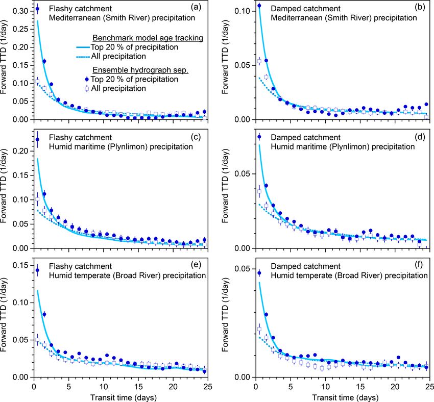
J. W. Kirchner: Ensemble hydrograph separation                                                                                 305

across an ensemble of events or time steps, it does not answer     together as Qold . Conservative mixing implies that
the same question that traditional hydrograph separation does
(namely, how fractions of new and old water change over            Qj CQj = Qnewj Cnewj + Qoldj Coldj ,                         (5)
time during individual storm events). Instead, it can answer
                                                                   where CQ and Cnew are the tracer concentrations in the
new and different questions, such as how the average frac-
                                                                   stream and the new water, and Cold is the tracer signature
tions of new and old water vary with stream discharge or pre-
                                                                   of all other sources that contribute to streamflow. Combining
cipitation intensity, antecedent moisture, etc. The proposed
                                                                   Eqs. (4) and (5), we directly obtain
method is designed to provide insights into stormflow gener-
ation from regularly sampled time series, even if those time
                                                                   CQj = Fnewj Cnewj + 1 − Fnewj Coldj ,                     (6)
series have gaps and even if they are sampled at frequencies
much lower than the storm response timescale of the catch-         where Fnewj = Qnewj /Qj is the fractional contribution of
ment.                                                              Qnew to streamflow Q. Equation (6) can be rewritten as
   The purpose of this paper is to describe the method, doc-
ument its mathematical foundations, and test it against a          CQj − Coldj = Fnewj Cnewj − Coldj ,                    (7)
benchmark model, in which the method’s results can be ver-
ified by age tracking. Applications to real-world catchments       which in turn could be rearranged as a conventional mixing
will follow in future papers. Because the proposed method is       model (Eq. 3), with the important difference that the new
new and thus must be fully documented, several parts of the        and old water concentrations are time-varying rather than
presentation (most notably Sect. 4.2–4.4 and Appendix B)           constant. If we represent the old water composition using
necessarily contain strong doses of math. The math can be          the streamwater concentration during the previous time step,
skipped, or lightly skimmed, by those who only need a gen-         Eq. (7) becomes
eral sense of the analysis. A table of symbols is provided at      CQj − CQj −1 = Fnewj Cnewj − CQj −1 .

                                                                                                                            (8)
the end of the text.
                                                                      The lagged concentration CQj −1 serves as a reference
                                                                   level for measuring fluctuations in precipitation and stream-
2     Estimating new water fractions by ensemble
                                                                   flow tracer concentrations and the correlations between them.
      hydrograph separation
                                                                   Thus, it is not necessary that CQj −1 consists entirely of old
Here I propose a new type of hydrograph separation based on        water as defined in conventional hydrograph separations (i.e.,
correlations between tracer fluctuations in streamflow and in      groundwater or baseflow water). It is only necessary that
one or more end-members. This new approach to hydrograph           CQj −1 contains no new water (that is, no precipitation that fell
separation does not have the same goal as conventional hy-         during time step j ), and this condition is automatically met
drograph separation. It does not estimate the contributions of     because CQj −1 is measured during the previous time step.
end-members to streamflow for each time step (as in Eq. 3).        The net effect of CQj −1 is to factor out the legacy effects of
Instead, it estimates the average end-member contributions to      previous tracer inputs and to filter out long-term variations
streamflow over an ensemble of time steps – hence its name,        in CQ that could otherwise lead to spurious correlations with
ensemble hydrograph separation. The ensemble of time steps         Cnew .
may be chosen to reflect different catchment conditions and           The ensemble hydrograph separation approach is based on
thus used to map out how those catchment conditions influ-         the observation that Eq. (8) is almost equivalent to the con-
ence end-member contributions to streamflow.                       ventional linear regression equation,

                                                                   yj = β xj + α + εj , yj = CQj − CQj −1 ,
2.1    Basic equations
                                                                   xj = Cnewj − CQj −1 ,                                        (9)
I will first illustrate this approach with a simple example of
a time-varying mixing model. Let us assume that we have            where the intercept α and the error term εj can be viewed
measured tracer concentrations in streamflow, and in at least      as subsuming any bias or random error introduced by mea-
one contributing end-member, over an ensemble of time in-          surement noise, evapoconcentration effects, and so forth. The
tervals j . The simplest possible mass balance for the water       analogy between Eqs. (9) and (8) suggests that it may be
that makes up streamflow would be                                  possible to estimate the average value of Fnewj from the re-
                                                                   gression slope of a scatterplot of the streamflow concentra-
Qj = Qnewj + Qoldj ,                                        (4)    tion CQj against the new water concentration Cnewj , both
                                                                   expressed relative to the lagged streamflow concentration
where Qnew represents the water flux in streamflow Q that          CQj −1 .
originates from recent precipitation (or, potentially, any other      However, astute readers will notice an important differ-
end-member in which tracers can be measured) during time           ence between Eqs. (8) and (9): in Eq. (9), the regression
interval j . All other contributions to streamflow are lumped      slope β is a constant, whereas in Eq. (8) Fnewj varies from

www.hydrol-earth-syst-sci.net/23/303/2019/                                         Hydrol. Earth Syst. Sci., 23, 303–349, 2019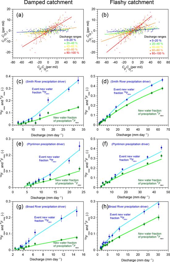
306 J. W. Kirchner: Ensemble hydrograph separation
one time step to the next. It is not obvious how an esti- 2.2 Uncertainties
mate of the (constant) slope β will be related to the (non-
constant) Fnewj or whether this relationship could be affected The uncertainty in Fnew , expressed as a standard error, can
by the other variables in Eq. (8). The answer to this question be written as
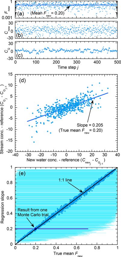
can be derived analytically and tested using numerical ex- q
2
1 − rxy
periments (see Appendix A). As explained in Appendix A, s
y
the regression slope in a scatterplot of CQj − CQj −1 versus SE (Fnew ) = SE β̂ = √
sx neff − 2
Cnewj − CQj −1 (Fig. A1d) will closely approximate the aver- s
age value of Fnewj (averaged over the ensemble of time steps β̂ 1
=√ 2
− 1, (11)
j ), under rather general conditions: neff − 2 rxy
1. The slope of the relationship between Fnewj and Cnewj − where sx and sy are the standard deviations of x and y, rxy is
CQj −1 , times the mean of Cnewj − CQj −1 , should be the correlation between them, and neff is the effective sample
small compared to the average Fnew . This will usu- size, which can be adjusted to account for serial correlation
ally be true for conservative tracers, for two reasons. in the residuals (Bayley and Hammersley, 1946; Brooks and
First, because all streamflow is ultimately derived from Carruthers, 1953; Matalas and Langbein, 1962):
new water, mass conservation implies that the mean of " #−1
n
Cnewj − CQj −1 should usually be small. Second, unless 1 + rsc 2 rsc 1 − rsc
neff ≈ nxy − , (12)
there is a correlation between storm size and tracer con- 1 − rsc nxy (1 − rsc )2
centration (not just between storm size and tracer vari-
ance), the slope of the relationship between Fnewj and where nxy is the number of pairs of xj and yj , and rsc is the
Cnewj −CQj −1 should also be small. Thus the product of lag-1 serial correlation in the regression residuals yj − β̂ xj −
these two small terms should be small. α. For large nxy , Eq. (12) can be approximated as (Mitchell
et al., 1966)
2. Points with large leverage in the scatterplot (i.e., with
1 − rsc
Cnewj − CQj −1 values far above and below the mean) neff ≈ nxy , (13)
1 + rsc
should not be systematically associated with either high
or low values of Fnewj . Such a systematic association is where for all positive rsc , Eq. (13) is conservative (it under-
unlikely unless large storms (which are likely to gener- estimates neff from Eq. 12), and for rsc = 0.5 and nxy > 50,
ate large new water fractions) are also associated with for example, Eqs. (12) and (13) differ by less than 3 %. If the
both very high and very low tracer concentrations. scatterplot of yj = CQj − CQj −1 versus xj = Cnewj − CQj −1
contains outliers, a robust fitting technique such as itera-
3. As expected for typical sampling and measurement er- tively reweighted least squares (IRLS) may yield more reli-
rors, the error term εj should not be strongly correlated able estimates of Fnew than ordinary least-squares regression.
with Cnewj − CQj −1 . However, the analyses presented here are based on outlier-
free synthetic data generated from a benchmark model (see
Thus the analysis in Appendix A shows that a reasonable es- Sect. 3), so in this paper I have used conventional least
timate of the ensemble average of Fnew should, under typi- squares (Eqs. 10–11) instead.
cal conditions, be obtainable from the regression slope β̂ of
a plot of xj = CQj − CQj −1 versus yj = Cnewj − CQj −1 (i.e., 2.3 New water fraction for time steps with
Eq. 9; Fig. A1d). precipitation
The least-squares solution of Eq. (9) can be expressed in
several equivalent ways. For consistency with the analysis The meaning of the new water fraction Fnew depends on how
that will be developed in Sect. 4 below, I will use the follow- the new water and streamwater are sampled. For example,
ing formulation, which is mathematically equivalent to those if the new water concentrations Cnew are measured in daily
more commonly seen: bulk precipitation samples and the stream water concentra-
tions CQ are measured in instantaneous grab samples taken
at the end of each 24 h precipitation sampling period, then
cov yj , xj
Fnew = β̂ = , (10) Fnew will estimate the average fraction of streamflow that
var xj is composed of precipitation from the preceding 24 h. If the
sampling interval is weekly instead of daily, then Fnew will
where β̂ is the least-squares estimate of β, and Fnew is the av- estimate the average fraction of streamflow that consists of
erage of the Fnewj over the ensemble of points j . Values of yj precipitation from the preceding week. This will generally
that lack a corresponding xj , or vice versa (due to sampling be larger than the Fnew calculated from daily sampling, for
gaps, for example, or lack of precipitation), are omitted. the obvious reason that on average more precipitation will
Hydrol. Earth Syst. Sci., 23, 303–349, 2019 www.hydrol-earth-syst-sci.net/23/303/2019/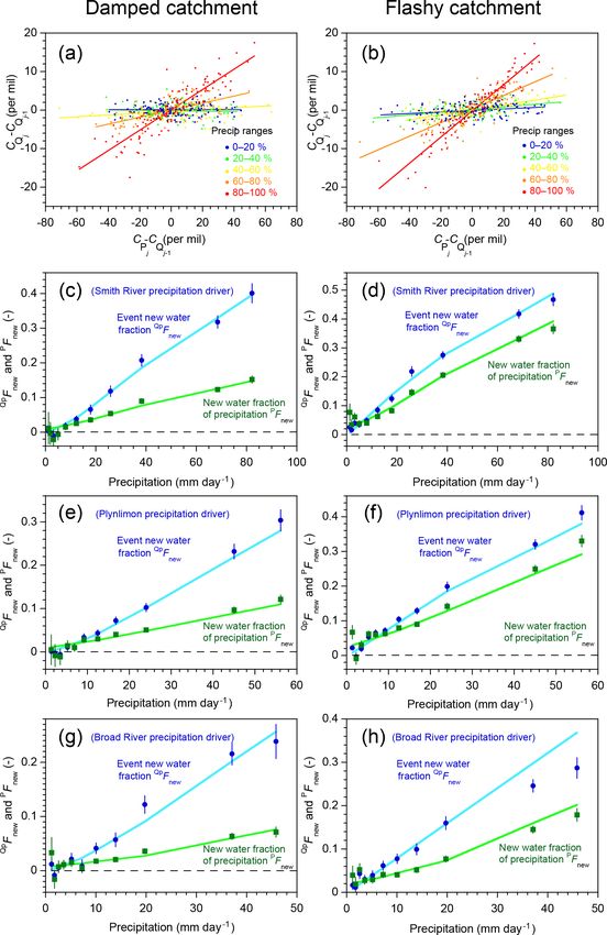
J. W. Kirchner: Ensemble hydrograph separation                                                                                          307

have fallen during the previous week than during the previ-
ous 24 h, so this precipitation will comprise a larger fraction                   P                                P
of streamflow. Also, if the weekly streamflow concentrations                            Qj xj                               Qj yj
                                                                                 j ∈(xy)                          j ∈(xy)
are measured in integrated composite samples rather than in-       x ∗(xy)   =      P           ,   y ∗(xy)   =      P              ,   (17)
stantaneous grab samples, then Fnew will estimate the frac-                                Qj                                Qj
                                                                                  j ∈(xy)                          j ∈(xy)
tion of same-week precipitation in average weekly stream-
flow rather than in the instantaneous end-of-week stream-          and the notation j ∈ (xy) indicates sums taken over all j for
flow. The general rule is: Fnew should generally estimate          which xj and yj are not missing. Equations (16)–(17) yield
whatever new water has been sampled as Cnew , expressed as         the slope coefficient for linear regressions like Eq. (9), but
a fraction of whatever streamflow has been sampled as CQ .         with each point weighted by the discharge Qj . We can de-
   In all of these cases, β̂ from Eq. (10) estimates the average   note the weighted regression slope β̂ ∗ as Qp Fnew
                                                                                                                  ∗ , the volume-
fraction of new water in streamflow during time steps with         weighted new water fraction of time intervals with precipita-
precipitation, because time steps without precipitation lack a     tion, where the asterisk indicates volume-weighting.
new water tracer concentration Cnewj and thus must be left            If, instead, one wants to estimate the new water fraction in
out from the regression in Eq. (9). Using Qp to denote dis-        all discharge (during periods with and without precipitation),
charge during periods with precipitation, we can represent         following the approach in Sect. 2.4 one simply rescales this
this event new water fraction as Qp Fnew .                         regression slope by the sum of discharge during time steps
                                                                   with precipitation, divided by total discharge:
2.4      New water fraction for all time steps

Periods without precipitation will inherently lack same-day        Q                        Qp np        Q p np
                                                                        ∗
                                                                       Fnew =Qp Fnew
                                                                                 ∗
                                                                                                  = β̂ ∗        ,                       (18)
(or same-week) precipitation in streamflow. Thus we can cal-                                Q  n         Q n
culate the average fraction of new water in streamflow during
all time steps, including those without precipitation, as          where Q Fnew
                                                                              ∗ is the volume-weighted new water fraction of

                                                                   all discharge, Qp Fnew
                                                                                        ∗  is the fitted regression slope β̂ from
Q                      np     np
    Fnew =Qp Fnew         = β̂ ,                           (14)    Eq. (16), Qp is the average discharge for time steps with pre-
                       n      n
                                                                   cipitation, Q is the average discharge for all time steps (in-
where Q Fnew is the new water fraction of all discharge,           cluding during rainless periods), and np /n is the fraction of
Qp F
     new is the new water fraction of discharge during time        time steps with rain.
steps with precipitation (as estimated by the regression slope        Because the volume-weighting will typically be uneven,
β̂, from Eq. 10), and np /n is the fraction of time steps that     the effective sample size will typically be smaller than n; for
have precipitation. The ratio np /n in Eq. (14) accounts for       example, in the extreme case that one sample had nearly all
the fact that during time steps without rain, the new water        the weight and the other samples had nearly none, the effec-
contribution to streamflow is inherently zero. The same ratio      tive sample size would be roughly 1 instead of nxy . Thus,
is also used to estimate the uncertainty in Q Fnew :               uncertainty estimates for these volume-weighted new wa-
                                         s                         ter fractions should take account of the unevenness of the
            n                QF          1                     weighting. One can account for uneven weighting by calcu-
      Q           p                 new
SE Fnew = SE β̂ = √                          2
                                                − 1.      (15)     lating the effective sample size, following Kish (1995), as
                 n               neff − 2 rxy
                                                                          P          2
2.5      Volume-weighted new water fractions                                 Qj (xy)
                                                                   neff = P           ,                                               (19)
                                                                              Q2j (xy)
The regression derived through Eqs. (4)–(9) gives each time
interval j equal weight. As a result, β̂ from Eq. (10) can
be interpreted as estimating the time-weighted average new         where the notation Qj (xy) indicates discharge at time steps j
water fraction. Alternatively, one can estimate the volume-        for which pairs of xj and yj exist. Equation (19) evaluates to
weighted new water fraction,                                       nxy (as it should) in the case of evenly weighted samples and
                                                               declines toward 1 (as it should) if a single sample has much
        P
            Qj yj − y ∗(xy) xj − x̄(xy)
                                     ∗                             greater weight than the others. To obtain an estimate of the
         j ∈(xy)                                                   effective sample size that accounts for both serial correlation
β̂ ∗ =                                  2   ,            (16)    and uneven weighting, one can multiply the expressions in
                         Qj xj − x ∗(xy)
                    P
                                                                   Eqs. (19) and (12) or (13). Combining these approaches, one
                   j ∈(xy)
                                                                   can estimate the standard error of Q Fnew
                                                                                                           ∗ as

where x ∗(xy) and ȳ(xy)
                    ∗    are the volume-weighted means of x                                                   s
                                                                                                     QF ∗
                                                                                          P
and y (averaged over all j for which xj and yj are not miss-
                                                                         Q    ∗
                                                                                           Qp  ∗       new   1
                                                                   SE        Fnew       = P SE β̂ = √              − 1,
ing),                                                                                       Q                   2
                                                                                                      neff − 2 rxy

www.hydrol-earth-syst-sci.net/23/303/2019/                                                 Hydrol. Earth Syst. Sci., 23, 303–349, 2019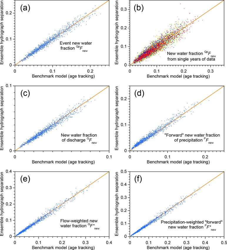
308                                                                       J. W. Kirchner: Ensemble hydrograph separation
                                   2
                                                                                   Qp
                        P
                           Qj (xy)      1 − rsc
                 neff = P                       ,        (20)         =Qp Fnew        ,                                    (24)
                            Q2j (xy)    1 + rsc                                    Pp

                                                                  where the “p” subscripts on the angled brackets indicate
where β̂ ∗ is the fitted regression slope from Eq. (16).          averages taken only over time intervals with precipitation.
                                                                  Whether this is a good approximation will depend on how
2.6     New water fraction of precipitation
                                                                  Pj , Qj , and Fnewj are distributed, and how they are cor-
One can also express the flux of new water as a fraction of       related with one another. By contrast, the approach out-
precipitation rather than discharge. Recently, von Freyberg et    lined in Eqs. (22)–(23) is based on the exact substitution of
al. (2018) have noted, in the context of conventional hydro-      Fnewj Qj /Pj for P Fnewj , which requires no approximations.
graph separation, that expressing event water as a proportion     The same substitution also leads to two other algebraically
of precipitation rather than discharge may lead to different      equivalent formulations of Eq. (22),
insights into catchment storm response. Analogously, within                               Pj
                                                                   CQj − CQj −1 = P Fnewj

the ensemble hydrograph separation framework we can esti-                                    Cnewj − CQj −1                  (25)
                                                                                          Qj
mate the new water fraction of precipitation, denoted P Fnew ,
as                                                                and

P                    Qp                                           Qj CQj − CQj −1 = P Fnewj Pj Cnewj − CQj −1 .

                                                                                                                             (26)
    Fnew = Qp Fnew        ,                                (21)
                     Pp
                                                                     But although Eqs. (22), (25), and (26) are algebraically
where Qp Fnew is the new water fraction of discharge during       equivalent, their statistical behavior is different when they
time steps with precipitation (as estimated by the regression     are used as regression equations to estimate the average value
slope β̂, from Eq. 10), and Qp and P p are the average dis-       of P Fnew . The regression estimate of P Fnew depends on the
charge and precipitation during these time steps. An alterna-     distributions of Pj , Qj , and Fnewj and their correlations with
tive strategy is to recast Eq. (8) by multiplying both sides by   each other, and benchmark testing shows that Eq. (22) yields
Qj /Pj , such that the Fnew on the right-hand side now ex-        reasonably accurate estimates of P Fnew , but Eqs. (25) and
presses new water as a fraction of precipitation,                 (26) do not. One can also note that the approach outlined in
                                                                Eq. (21) – the other approach that is successful in benchmark
Qj                         Qj
      CQj − CQj −1 =           Fnewj Cnewj − CQj −1               tests – represents an ad hoc time averaging of Pj and Qj in
 Pj                         Pj                                    Eq. (22), because it is formally equivalent to
                        P

                       = Fnewj Cnewj − CQj −1 .            (22)
                                                                  Qp
                                                                        CQj − CQj −1 = P Fnewj Cnewj − CQj −1 .

  This yields a linear regression similar to Eq. (9), but with                                                               (27)
                                                                  Pp
yj rescaled,
                          Qj                                        The precise interpretation of P Fnew depends on how
yj = β xj + α + εj , yj =    CQj − CQj −1 ,                       streamflow is sampled. If the streamflow tracer concentra-
                          Pj
                                                                 tions come from integrated composite samples over each day
xj = Cnewj − CQj −1 ,                                      (23)   or week, then P Fnew can be interpreted as the fraction of
                                                                  precipitation that becomes same-day or same-week stream-
where the regression slope β̂, which can be calculated from       flow. If the streamflow tracer concentrations instead come
Eq. (10) with the new values yj , should approximate the av-      from instantaneous grab samples (as is more typical), then
erage new water fraction of precipitation P Fnew .                PF
                                                                     new can be interpreted as the rate of new water discharge
   The approaches represented by Eqs. (21) and (22)–(23) are      at that time (typically the end of the precipitation sampling
not equivalent. Equation (21) is based on the ad hoc assump-      interval), as a fraction of the average rate of precipitation.
tion – which is verified by the benchmark tests in Sect. 3.3–     Adapting terminology from the literature of transit time dis-
3.5 – that the average of P Fnewj (new water in streamflow, as    tributions (TTDs), we can call P Fnew the “forward” new wa-
a fraction of precipitation) should approximate the average       ter fraction because it represents the fraction of precipitation
Fnewj (new water in streamflow, as a fraction of discharge),      that will exit as streamflow soon (during the same time step),
rescaled by the ratio of average discharge Qpj to average pre-    and call Qp Fnew and Q Fnew “backward” new water fractions
cipitation Ppj . This is only an approximation, of course; it     because they represent the fraction of streamflow that entered
relies on the approximation that appears in the middle of the     the catchment a short time ago. Although the backward new
following chain of expressions:                                   water fraction of discharge comes in two forms (Qp Fnew or
                                                                  QF
                                                                      new ), depending on whether one includes or excludes rain-

                                Qj
                                               Qj p
P
    Fnew =   P
                 Fnew p = Fnewj      ≈ hFnew ip                   less periods, the forward new water fraction P Fnew can only
                                Pj p            Pj p              be defined for time steps with precipitation (otherwise P Fnew

Hydrol. Earth Syst. Sci., 23, 303–349, 2019                                      www.hydrol-earth-syst-sci.net/23/303/2019/
J. W. Kirchner: Ensemble hydrograph separation                                                                                       309

represents the ratio between zero new water and zero precip-
itation and thus is undefined).                                                   P                                P
   Readers should keep in mind that although P Fnew repre-                              Pj xj                            Pj yj
                                                                                 j ∈(xy)                          j ∈(xy)
sents the fraction of precipitation that becomes same-day (or      x ∗(xy)   =      P           ,   y ∗(xy)   =      P           ,   (30)
                                                                                           Pj                               Pj
same-week) streamflow, different fractions of precipitation                       j ∈(xy)                          j ∈(xy)
may leave the catchment the same day (or week) by other
pathways, most notably by evapotranspiration. One could            and where the regression slope β̂ ∗ approximates the
also estimate P Fnew for water that leaves the catchment by        precipitation-weighted average forward new water fraction
evapotranspiration if one had tracer time series for evapo-        PF ∗ .
                                                                      new
transpiration fluxes, but at present such time series are not
available. Thus, to echo the principle outlined in Sect. 2.3
above, the new water fraction of precipitation does not repre-     3     Testing ensemble hydrograph separation with a
sent the forward new water fraction for all possible pathways,           simple non-stationary benchmark model
but only whatever pathway has been sampled.
                                                                   3.1       Benchmark model
2.7      Volume-weighted new water fraction of
         precipitation                                             To test the methods outlined in Sect. 2 above, I use synthetic
                                                                   data generated by a simple two-box lumped-parameter catch-
The new water fraction of precipitation as estimated by            ment model. This model is documented in greater detail in
Eq. (21) is a time-weighted average, in which each day with        Kirchner (2016a) and will be described only briefly here. As
precipitation counts equally. One may also want to estimate        shown in Fig. 1a, drainage L from the upper box is a power
the volume-weighted new water fraction of precipitation,           function of the storage Su within the box; a fraction η of this
which we can denote as P Fnew∗ , in keeping with the naming
                                                                   drainage flows directly to streamflow, and the complemen-
conventions used above. We can estimate P Fnew  ∗ at least two
                                                                   tary fraction 1 − η recharges the lower box, which drains to
different ways. The first method involves recognizing that we      streamflow at a rate Ql that is a power function of its storage
are seeking the ratio between the total volume of new water        Sl . The model’s behavior is determined by five parameters:
– that is, same-day precipitation reaching streamflow – and        the equilibrium storage levels Su, ref and Sl, ref in the upper
the total volume of precipitation. This will equal the volume-     and lower boxes, their drainage exponents bu and bl , and the
weighted new water fraction of discharge (total new water          drainage partitioning coefficient η. For simplicity, evapotran-
divided by total discharge, which has already been derived         spiration is not explicitly simulated; instead, the precipita-
in Sect. 2.5 above), rescaled by the ratio of total discharge to   tion inputs can be considered to be effective precipitation,
total precipitation:                                               net of evapotranspiration losses. Discharge from both boxes
                                                                   is assumed to be non-age selective, meaning that discharge
P                      Q                     Qp np
     ∗
    Fnew = Q Fnew
              ∗
                             =   Qp    ∗
                                      Fnew         ,       (28)    is taken proportionally from each part of the age distribu-
                        P                    P n                   tion. Tracer concentrations and mean ages are tracked under
                                                                   the assumption that the boxes are each well mixed but also
where Q and P are the average rates of discharge and pre-
                                                                   distinct from one another, so their tracer concentrations and
cipitation (averaged over all time steps), Qp is the average
                                                                   water ages will differ. Water ages and tracer concentrations
discharge on days with rain, and np /n is the fraction of time
                                                                   are also tracked in daily age bins up to an age of 70 days,
steps with rain. An alternative strategy, which yields nearly
                                                                   and mean water ages are tracked in both the upper and lower
equivalent results in benchmark tests, precipitation-weights
                                                                   boxes.
the regression for P Fnew (Eq. 22), yielding
                                                                       The model operates at a daily time step, with the storage
                                                               evolution of the lower box calculated by a weighted combi-
             Pj yj − y ∗(xy) xj − x ∗(xy)
         P
         j ∈(xy)
                                                                   nation of the partly implicit trapezoidal method (for greater
β̂ ∗ =                                  2            ,           accuracy) and the fully implicit backward Euler method (for
                         Pj xj − x ∗(xy)
                    P
                                                                   guaranteed stability). Unlike in Kirchner (2016a), here the
                   j ∈(xy)                                         storage evolution of the upper box is calculated by forward
     Qj                                                          Euler integration at 50 sub-daily time steps of 0.02 days
yj =    CQj − CQj −1 , xj = Cnewj − CQj −1 ,               (29)
     Pj                                                            (roughly 30 min) each. At this time step, forward Euler in-
                                                                   tegration is stable across the entire parameter ranges used in
where x ∗(xy) and y ∗(xy) are the precipitation-weighted means     this paper and is more accurate than daily time steps of trape-
of x and y (averaged over all j for which xj and yj are not        zoidal or backward Euler integration (which are still ade-
missing),                                                          quate for the lower box, where storage volumes change more
                                                                   slowly). Following Kirchner (2016a), the model is driven
                                                                   with three different real-world daily rainfall time series, rep-

www.hydrol-earth-syst-sci.net/23/303/2019/                                                 Hydrol. Earth Syst. Sci., 23, 303–349, 2019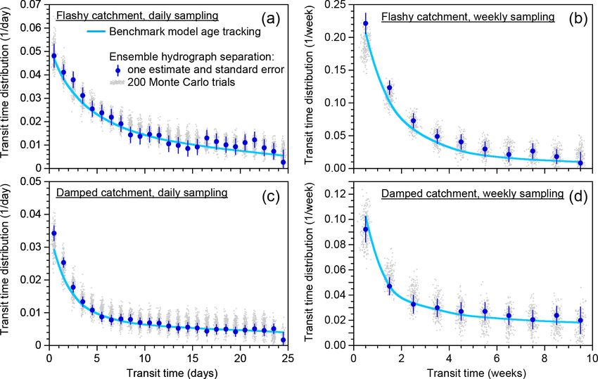
310                                                                                J. W. Kirchner: Ensemble hydrograph separation

Figure 1. Schematic diagram of the benchmark model (a), with 2-year excerpts from illustrative simulations of its behavior (b–i). Model
parameters for simulations of damped catchment response (b, d, f, h) are Su, ref = 100 mm, Sl, ref = 1000 mm, bu = 10, bl = 3, and η = 0.3.
For simulations of flashy catchment response (c, e, g, i), all but one of the parameters are the same; only η is changed to 0.8 and a different
random realization of precipitation isotopes is used. The same daily precipitation time series (Smith River, Mediterranean climate) is used
in both cases. The isotopic composition of streamflow exhibits complex dynamics over multiple timescales (blue line in d, e), as dominance
shifts between the upper and lower boxes (green and orange lines, respectively, in d, e). Like the discharge and its isotopic composition, the
fraction of discharge comprised of same-day precipitation (the new water fraction of discharge, Q Fnew , f, g) exhibits complex nonstationary
dynamics. Nonetheless, its long-term average (dashed blue line) is well predicted by ensemble hydrograph separation (solid blue line); the
same is true of the discharge-weighted average (dashed and solid red lines). The fraction of precipitation appearing in same-day discharge
(the forward new water fraction, P Fnew , h, i) is somewhat less variable, but both its average and precipitation-weighted average are also well
predicted by ensemble hydrograph separation (solid and dashed blue and red lines). In several cases the dashed and solid lines cannot be
distinguished because they overlap.

resenting a range of climatic regimes: a humid maritime cli-              tracer. The model is then run for a 1-year spin-up period; the
mate with frequent rainfall and moderate seasonality (Plyn-               results reported here are from 5-year simulations following
limon, Wales; Köppen climate zone Cfb), a Mediterranean                   this spin-up period.
climate marked by wet winters and very dry summers (Smith                    For the simulations shown here, the drainage exponents
River, California, USA; Köppen climate zone Csb), and a                   bu and bl are randomly chosen from uniform distributions of
humid temperate climate with very little seasonal variation               logarithms spanning the range of 1–20, and the partitioning
in average rainfall (Broad River, Georgia, USA; Köppen cli-               coefficient η is randomly chosen from a uniform distribu-
mate zone Cfa). Synthetic daily precipitation tracer (deu-                tion ranging from 0.1 to 0.9. The reference storage levels
terium) concentrations are generated randomly from a nor-                 Su,ref and Sl, ref are randomly chosen from a uniform dis-
mal distribution with a standard deviation of 20 ‰ and a lag-             tribution of logarithms spanning the ranges of 50–200 mm
1 serial correlation of 0.5, superimposed on a seasonal cy-               and 200–2000 mm, respectively. These parameter distribu-
cle with an amplitude of 10 ‰. The model is initialized at                tions encompass a wide range of possible behaviors, includ-
the equilibrium storage levels Su, ref and Sl, ref , with age dis-        ing both strong and damped response to rainfall inputs.
tributions and tracer concentrations corresponding to steady-                I illustrate the behavior of the model using two particular
state equilibrium values at the mean input fluxes of water and            parameter sets, one that gives damped response to precipi-

Hydrol. Earth Syst. Sci., 23, 303–349, 2019                                                www.hydrol-earth-syst-sci.net/23/303/2019/
J. W. Kirchner: Ensemble hydrograph separation                                                                               311

tation (Su, ref = 100 mm, Sl, ref = 1000 mm, bu = 10, bl = 3,    trivial to model a tracer time series assuming that new water
and η = 0.3) and one that gives a more rapid response (the       constituted a fixed fraction of discharge, and then demon-
same parameters, except η = 0.8). These parameter values         strate that this fraction can be retrieved from the tracer be-
are not preferable to others in any particular way; they sim-    havior. What Fig. 1 demonstrates is much less obvious, and
ply generate strongly contrasting streamflow and tracer re-      more important: that even when the new water fraction is
sponses that look plausible as examples of small catchment       highly dynamic and nonstationary, an appropriate analysis of
behavior. They can be interpreted as the behavior of two con-    tracer behavior can accurately estimate its mean.
trasting model catchments, which for simplicity (but with
some linguistic imprecision) I will call the “damped catch-      3.3   Benchmark tests: random parameter sets
ment” and the “flashy catchment”, as shorthand for “model
catchment with parameters giving more damped response”           This result holds not just for the two parameter sets shown in
and “model catchment with parameters giving more flashy          Fig. 1, but throughout the parameter ranges that are tested in
response”.                                                       the benchmark model. The scatterplots shown in Fig. 2 show
   The model also simulates the sampling process and its as-     new water fractions estimated by ensemble hydrograph sep-
sociated errors. I assume that tracer concentrations cannot      aration, compared to the true average new water fractions de-
be measured when precipitation rates are below a threshold       termined by age tracking in the benchmark model, for 1000
of Pthreshold =1 mm day−1 , such that tracer samples below       random parameter sets spanning the parameter ranges de-
this threshold will be missing. I further assume that 5 % of     scribed in Sect. 3.1. Figure 2 shows that ensemble hydro-
all other precipitation tracer measurements, and 5 % of all      graph separation yields reasonably accurate estimates of av-
streamflow tracer measurements, will be lost at random times     erage event new water fractions (Fig. 2a, b), new water frac-
due to sampling or analysis failures. I have also added Gaus-    tions of discharge (Fig. 2c) and precipitation (Fig. 2d), and
sian random errors (with a standard deviation of 1 ‰) to all     volume-weighted new water fractions (Fig. 2e, f). Estimates
tracer measurements.                                             derived from single years of data (Fig. 2b) understandably
                                                                 exhibit greater scatter than those derived from 5 years of
3.2   Benchmark model behavior                                   data (Fig. 2a), but in all of the plots shown in Fig. 2 there
                                                                 is no evidence of significant bias (the data clouds cluster
Panels b–i of Fig. 1 show 2 years of simulated daily behav-      around the 1 : 1 lines). The scatter of the points around the
ior driven by the Smith River daily precipitation record ap-     1 : 1 line generally agrees with the standard errors estimated
plied to the damped and flashy catchment parameter sets. The     from Eqs. (11), (15), and (20), suggesting that these uncer-
simulated stream discharge responds promptly to rainfall in-     tainty estimates are also reliable.
puts, and unsurprisingly the discharge response is larger in        Mean transit times have often been estimated in the catch-
the flashy catchment (Fig. 1b, c). The streamflow isotopic       ment hydrology literature, often under the assumption that
response is strongly damped in both catchments, with iso-        they should also be correlated with other timescales of catch-
tope ratios between events returning to a relatively stable      ment transport and mixing as well. This naturally leads to
baseline value composed mostly of discharge from the lower       the question, in the context of the present study, of whether
box (Fig. 1d, e). Like the stream discharge and the isotope      there is a systematic relationship between mean transit times
tracer time series, the instantaneous new water fractions (de-   and new water fractions, such that they could potentially be
termined by age tracking within the model) also exhibit com-     predicted from one another. The benchmark model allows a
plex nonstationary dynamics (Fig. 1f–i). Despite the com-        direct test of this conjecture, because it tracks mean water
plexity of the modeled time-series behavior, ensemble hydro-     ages as well as new water fractions. Figure 3a shows that,
graph separation (Eqs. 14, 18, 21, and 28) accurately predicts   across the 1000 random parameter sets from Fig. 2, the rela-
the averages of these new water fractions, both unweighted       tionship between new water fractions and mean transit times
and time-weighted, as can be seen by comparing the dashed        is a nearly perfect shotgun blast: mean transit times vary
and solid lines (which sometimes overlap) in Fig. 1f–i.          from about 40 to 400 days and new water fractions vary from
   It should be emphasized that the ensemble hydrograph          nearly zero to nearly 0.1, with almost no correlation between
separation and the benchmark model are completely inde-          them. Both of these quantities are estimated from age track-
pendent of one another. The ensemble hydrograph separa-          ing in the benchmark model, so their lack of any systematic
tion does not know (or assume) anything about the internal       relationship does not arise from difficulties in estimating ei-
workings of the benchmark model; it knows only the input         ther of them from tracer data. It instead arises because the up-
and output water fluxes and their isotope signatures. This is    per tails of transit time distributions (reflecting the amounts
crucial for it to work in the real world, where any particu-     of streamflow with very old ages) exert strong influence on
lar assumptions about the processes driving runoff could po-     mean transit times, but have no effect on new water fractions
tentially be violated. Likewise, the benchmark model is not      (reflecting same-day streamflow).
designed to conform to the assumptions underlying the en-           I have recently proposed the “young water fraction”, the
semble hydrograph separation method. It would be relatively      fraction of streamflow younger than about 2.3 months, as a

www.hydrol-earth-syst-sci.net/23/303/2019/                                       Hydrol. Earth Syst. Sci., 23, 303–349, 2019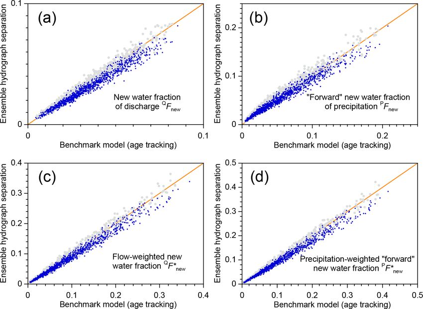
312                                                                               J. W. Kirchner: Ensemble hydrograph separation

Figure 2. New water fractions predicted from tracer dynamics using ensemble hydrograph separation, compared to averages of time-varying
new water fractions determined from age tracking in the benchmark model. Diagonal lines show perfect agreement. Each scatterplot shows
1000 points, each of which represents an individual catchment, with its own individual random set of model parameters (i.e., catchment
characteristics), randomly generated precipitation tracer time series, and random set of measurement errors and missing values (see Sect. 3.1).
The daily precipitation amounts are the same (Smith River time series; Mediterranean climate) in each case. The event new water fraction (a,
b) is the average fraction of new (same-day) water in streamflow during time steps with precipitation, as described in Sect. 2.3. Panel (a)
shows event new water fractions estimated from 5 years of simulated tracer data; panel (b) shows the same quantity estimated from single
years (each year is denoted by a different color). Averaging over the 5 years reduces both the range and the scatter, compared to the single-
year estimates. The new water fraction of discharge (c) is the fraction of same-day precipitation in streamflow, averaged over all time steps
including rainless periods (Eq. 14, Sect. 2.4); its flow-weighted counterpart (e) is calculated using Eqs. (16)–(18) of Sect. 2.5. The forward
new water fraction (the fraction of precipitation that becomes same-day streamflow; d) is calculated using Eq. (21), and its precipitation-
weighted counterpart (f) is calculated using Eq. (28). In all cases there is little evidence of bias, and the scatter around the 1 : 1 line is
relatively small.

more robust metric of water age than the mean transit time                stant, which is not the case for the 1000 random parameter
(Kirchner, 2016b). Figure 3b shows that, like the mean transit            sets considered here and is not likely to be true in real-world
time, the young water fraction is also a poor predictor of the            catchments either.
new water fraction, beyond the obvious constraint that new
water (≤1 day old) must be a small fraction of young water                3.4   Benchmark tests: weekly tracer sampling
(≤ 69 days old). The new water fraction will only be corre-
lated with the young water fraction or mean transit time if the           Many long-term water isotope time series have been sampled
shape of the underlying transit time distribution is held con-            at weekly intervals. Can new water fractions be estimated re-
                                                                          liably from such sparsely sampled records? To find out, I ag-

Hydrol. Earth Syst. Sci., 23, 303–349, 2019                                               www.hydrol-earth-syst-sci.net/23/303/2019/
J. W. Kirchner: Ensemble hydrograph separation 313
Figure 3. Average new water fractions (same-day precipitation in streamflow) for the 1000 simulated catchments (i.e., 1000 model parameter
sets) shown in Fig. 2, compared to the catchment mean transit time and the young water fraction Fyw (the fraction of streamflow younger
than 2.3 months). All values plotted here are determined from age tracking within the benchmark model, and thus are true values, without
any errors associated with estimating these quantities from tracer data. Neither mean transit time nor the young water fraction can reliably
predict the fraction of new water in streamflow.
gregated the benchmark model’s daily time series to weekly termined by age tracking in the benchmark model, analo-
intervals, volume-weighting the isotopic composition of pre- gous to Fig. 2 but for weekly instead of daily sampling. The
cipitation to simulate the effects of weekly bulk precipitation weekly new water fractions are larger than the daily ones,
sampling, and subsampling streamflow isotopes every sev- for the reasons described above, and exhibit more scatter be-
enth day to simulate weekly grab sampling. I then performed cause they are based on fewer data points than their daily
ensemble hydrograph separation on the aggregated weekly counterparts are. A small overestimation bias is visually ev-
data, using the methods presented in Sect. 2. ident in Fig. 2d and an even smaller underestimation bias is
Figure 4 shows the behavior of the benchmark model at evident in Fig. 2c. These reservations notwithstanding, Fig. 5
weekly resolution for both the damped and flashy catch- shows that ensemble hydrograph separation can reliably pre-
ments. At the weekly timescale, the benchmark model ex- dict new water fractions of both discharge and precipitation,
hibits complex nonstationary dynamics in discharge (panels with and without volume-weighting, based on weekly tracer
a, b), water isotopes (panels c, d), and new water fractions samples.
(panels e, h). Nonetheless – and even though the weekly sam-
pling timescale is much longer than the timescales of hydro-
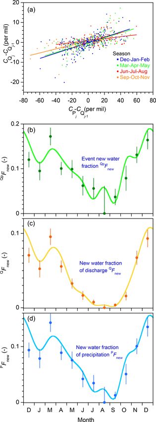
3.5 Variations in new water fractions with discharge,
logic response in the system – ensemble hydrograph separa-
precipitation, and seasonality
tion yields reasonable estimates for the mean new water frac-
tions of both precipitation and discharge (both unweighted
and flow-weighted), as one can see by comparing the dashed Ensemble hydrograph separation does not require continuous
and solid lines in Fig. 4e–h. data as input, so it can be used to estimate Fnew values for
A comparison of Figs. 1 and 4 shows that the isotopic (potentially discontinuous) subsets of a time series that re-
signature of precipitation is less variable among the weekly flect conditions of particular interest. For example, if we split
samples than among the daily samples, reflecting the fact that the time series shown in Fig. 1 into several discharge ranges,
the weekly bulk samples of precipitation will inherently aver- we can see that at higher flows, tracer fluctuations in the
age over the sub-weekly variability in daily rainfall. By con- stream are more strongly correlated with tracer fluctuations
trast, the weekly grab samples of streamflow lose all informa- in precipitation (Fig. 6a, b). Each of the regression slopes in
tion about what is happening on shorter timescales. The new Fig. 6a, b defines the event new water fraction Qp Fnew for
water fractions calculated from the weekly data are distinctly the corresponding discharge range. Repeating this analysis
higher than those calculated from the daily data, owing to the for each 10 % interval of the discharge distribution (0th–10th
fact that the definition of new water depends on the sampling percentile, 10th–20th percentile, etc.), plus the 95th–100th
frequency: the proportion of water ≤ 7 days old (new un- percentile, yields the profiles of Qp Fnew as functions of dis-
der weekly sampling) can never be less than the proportion charge, as shown by the blue dots in Fig. 6c–h. The green
≤ 1 day old (new under daily sampling). squares show the corresponding forward new water fractions
PF
Figure 5 shows scatterplots comparing new water fractions new for comparison. The light blue and light green lines
estimated by ensemble hydrograph separation and those de- show the corresponding true new water fractions determined
by age tracking in the benchmark model.
www.hydrol-earth-syst-sci.net/23/303/2019/ Hydrol. Earth Syst. Sci., 23, 303–349, 2019314 J. W. Kirchner: Ensemble hydrograph separation Figure 4. Illustrative simulations of weekly water fluxes, deuterium concentrations, and new water fractions. The benchmark model, pre- cipitation forcing, and parameter values are identical to those in Fig. 1. Although the isotope tracer concentrations and new water fractions exhibit complex nonstationary dynamics, ensemble hydrograph separation yields reasonable estimates of the average backward and forward weekly new water fractions, as shown in (e, f) and (g, h), respectively. Panels (a) and (b) show weekly average rates of precipitation and discharge. Panels (c) and (d) show the weekly volume-weighted isotopic composition of precipitation (mimicking what would be collected in a weekly rain sample) and the instantaneous composition of discharge at the end of each week (mimicking what would be collected in a weekly grab sample). Panels (e) and (f) show the fraction of discharge that is composed of same-week precipitation (the weekly new water fraction; yellow lines), as determined from model age tracking, and its long-term average (dashed blue line), compared to the new water fraction predicted by ensemble hydrograph separation (solid blue line) from the weekly samples shown in (b). Panels (g) and (h) show the fraction of precipitation that becomes same-week discharge (the weekly new water fraction of precipitation, or forward new water fraction, yellow lines), as determined from model age tracking, and its long-term average (dashed blue line), compared to the new water fraction predicted by ensemble hydrograph separation (solid blue line). Discharge-weighted and precipitation-weighted average new water fractions, and their predicted values, are shown by red solid and dashed lines. If, instead, we split the time series shown in Fig. 1 into ward new water fractions are typically smaller than event subsets reflecting ranges of precipitation rates rather than new water fractions, because during storms the rainfall rate discharge, we obtain Fig. 7. Figure 7 is a counterpart to is higher than the streamflow rate, so the ratio between same- Fig. 6, but with Qp Fnew and P Fnew plotted as functions of day streamflow and the total rainfall rate (P Fnew ) will neces- rainfall rates rather than discharge. The two figures exhibit sarily be smaller than the ratio between same-day streamflow broadly similar behavior. Unsurprisingly, new water frac- and the total streamflow rate (Qp Fnew ). Exceptions to this rule tions are higher at higher discharges and rainfall rates, be- arise when rainfall rates are lower than discharge rates, such cause under these conditions a higher fraction of discharge as during periods of light rainfall while streamflow is still un- comes from the upper box, which has younger water. For- dergoing recession from previous heavy rain. Thus the green Hydrol. Earth Syst. Sci., 23, 303–349, 2019 www.hydrol-earth-syst-sci.net/23/303/2019/
J. W. Kirchner: Ensemble hydrograph separation                                                                                             315

Figure 5. New water fractions estimated from weekly tracer dynamics using ensemble hydrograph separation, compared to averages of
time-varying new water fractions determined from age tracking in the benchmark model. Plots are similar to those in Fig. 2, except here they
are derived from simulated weekly sampling of tracer concentrations in precipitation and streamflow. Diagonal lines show perfect agreement.
Each scatterplot shows 1000 points, each representing an individual random set of parameters, a randomly generated precipitation tracer time
series, and a random set of measurement errors and missing values (see Sect. 3.1). The daily precipitation amounts are the same (Smith River
time series) in each case. The event new water fraction (a, b) is the average fraction of new (same-day) water in streamflow during time steps
with precipitation, as described in Sect. 2.3. Panel (a) shows event new water fractions estimated from 5 years of simulated weekly tracer
data; panel (b) shows the same quantity estimated from single years of simulated weekly tracer data (each year is denoted by a different
color). Averaging over the 5 years reduces scatter compared to the individual-year estimates. The new water fraction of discharge (c) is the
fraction of same-day precipitation in streamflow, averaged over all time steps including rainless periods (Eq. 14, Sect. 2.4); its flow-weighted
counterpart (e) is calculated using Eqs. (16)–(18) of Sect. 2.5. The forward new water fraction (the fraction of precipitation that becomes
same-day streamflow; d) is calculated using Eq. (21), and its precipitation-weighted counterpart (f) is calculated using Eq. (28). There is only
slight visual evidence of bias, and the scatter around the 1 : 1 line is small compared to the range spanned by the new water fractions.

and blue curves cross over one another at the left-hand edges             rainfall forcing. Second, different catchment parameters (dif-
of Fig. 7c–h, whereas in Fig. 6c–h they do not.                           ferent columns in Fig. 6) and different precipitation forcings
   Three conclusions can be drawn from Figs. 6 and 7. First,              (different rows in Fig. 6) yield different patterns in the rela-
in these model catchments, new water fractions vary dramat-               tionships between the new water fractions Qp Fnew and P Fnew
ically between low flows and high flows, and between low                  on the one hand and precipitation and discharge on the other.
and high precipitation rates, with the event new water frac-              And third, these patterns are accurately quantified by ensem-
tion Qp Fnew and the forward new water fraction P Fnew di-                ble hydrograph separation, which matches the age-tracking
verging from one another more at higher flows and higher

www.hydrol-earth-syst-sci.net/23/303/2019/                                                  Hydrol. Earth Syst. Sci., 23, 303–349, 2019
You can also read