Predicting the Trend of Stock Market Index Using the Hybrid Neural Network Based on Multiple Time Scale Feature Learning - MDPI
←
→
Page content transcription
If your browser does not render page correctly, please read the page content below
applied
           sciences
Article
Predicting the Trend of Stock Market Index Using the
Hybrid Neural Network Based on Multiple Time
Scale Feature Learning
Yaping Hao * and Qiang Gao
 School of Electronic and Information Engineering, Beihang University, Beijing 100191, China;
 gaoqiang@buaa.edu.cn
 * Correspondence: haoyaping@buaa.edu.cn; Tel.: +86-138-1096-8583

 Received: 25 April 2020; Accepted: 4 June 2020; Published: 7 June 2020

 Abstract: In the stock market, predicting the trend of price series is one of the most widely investigated
 and challenging problems for investors and researchers. There are multiple time scale features in
 financial time series due to different durations of impact factors and traders’ trading behaviors. In this
 paper, we propose a novel end-to-end hybrid neural network, a model based on multiple time scale
 feature learning to predict the price trend of the stock market index. Firstly, the hybrid neural network
 extracts two types of features on different time scales through the first and second layers of the
 convolutional neural network (CNN), together with the raw daily price series, reflect relatively short-,
 medium- and long-term features in the price sequence. Secondly, considering time dependencies
 existing in the three kinds of features, the proposed hybrid neural network leverages three long
 short-term memory (LSTM) recurrent neural networks to capture such dependencies, respectively.
 Finally, fully connected layers are used to learn joint representations for predicting the price trend.
 The proposed hybrid neural network demonstrates its effectiveness by outperforming benchmark
 models on the real dataset.

 Keywords: stock market index trend prediction; multiple time scale features; deep learning;
 convolutional neural network; long short-term memory neural network

1. Introduction
     The trend of the stock market index refers to the upward or downward movements of price series
in the future. Accurately predicting the trend of the stock market index can help investors avoid risks
and obtain higher returns in the stock exchange [1]. Hence, it has become a hot field and attracted
many researchers’ attention.
     Unitl now, many techniques and various models have been applied to predict the stock market
index. Such as traditional statistical models [2,3], machine learning methods [3,4], artificial neural
networks (ANNs) [5–8], etc. With the development of deep learning, there are lots of methods based
on deep learning used for stock forecasting and have drawn some essential conclusions [9–22].
     The above studies were conducted from single time scale features of the stock market index,
but it is also meaningful for studying from multiple time scale features. There are multiple time
scale features in the stock market index. On the one hand, the stock market is affected by many
factors such as economic environment, political policy, industrial development, market news, natural
factors and so on. And the durations of factors are different from each other. On the other hand, each
investor has a different investment cycle, such as long- and short-term investment. Therefore, we can
observe the features of multiple time scales in the stock market index. Among them, the features of
a long time scale can reflect the long-term trend of the price, while the features of short time scale

Appl. Sci. 2020, 10, 3961; doi:10.3390/app10113961                                www.mdpi.com/journal/applsci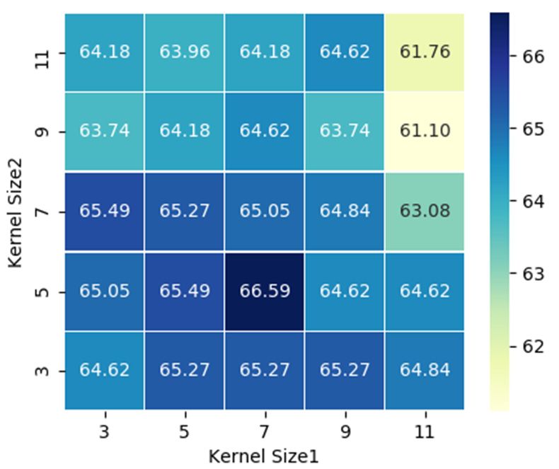
Appl. Sci. 2020, 10, 3961 2 of 14
Appl. Sci. 2020, 10, x FOR PEER REVIEW 2 of 15
can reflect the short-term fluctuation of the price. The combination of multi-scale features facilitates
the short-term
accurate fluctuation of the price. The combination of multi-scale features facilitates accurate
prediction.
prediction.
In recent years, the convolutional neural network (CNN) has shown high power in feature
In recent
extraction. years,
Inspired bythe convolutional
existing neural
research, we use network
a CNN to(CNN)extracthas showntime
multiple high power
scale in feature
features for more
extraction. Inspired by existing research, we use a CNN to extract multiple time scale
comprehensive learning of price sequences. For instance, the daily closing price series in Figure features for 1a
more comprehensive learning of price sequences. For instance, the daily closing price series in Figure
is learned by a two-layer convolutional neural network. The outputs of the two layers of the CNN
1a is learned by a two-layer convolutional neural network. The outputs of the two layers of the CNN
are called Feature map1 and Feature map2, respectively. As illustrated in Figure 1b, each point of the
are called Feature map1 and Feature map2, respectively. As illustrated in Figure 1b, each point of the
feature map corresponds to a region of the original price series (termed the receptive field [23]), and it
feature map corresponds to a region of the original price series (termed the receptive field [23]), and
can be considered as the description for the region. Due to different receptive fields, Feature map1
it can be considered as the description for the region. Due to different receptive fields, Feature map1
and Feature map2 describe the input price series from two-time scales. Compared with Feature map1,
and Feature map2 describe the input price series from two-time scales. Compared with Feature map1,
Feature
Featuremap2
map2describes
describes the
the original pricesequence
original price sequenceon ona alarger
largertime
time scale.
scale. Therefore,
Therefore, wewe regard
regard the the
outputs of different layers of the CNN as features of varying time scales of the original price
outputs of different layers of the CNN as features of varying time scales of the original price series. series.
Feature map 2
MaxPooling 1D
Feature map 2
Conv 1D
Feature map 1 Feature map 1
MaxPooling 1D
Conv 1D Input
Input {x1 , x2 , x3 , xT } x1 x2 x3 x4 x5 x6 x7 x8 x9 x10 xT − 2 xT −1 xT
(a) (b)
Figure1.1.An
Figure Anexample
example showing
showing that
that CNN
CNNcancanextract
extractfeatures
featuresofofdifferent time
different timescales. (a) (a)
scales. TheThe
dailydaily
closing price series learned by a convolutional neural network; (b) Description of the time scale
closing price series learned by a convolutional neural network; (b) Description of the time scale of of the
features.
the features.
Meanwhile,the
Meanwhile, the Long
Long Short-Term
Short-Term Memory
Memory(LSTM)
(LSTM)network
networkworksworkswell onon
well sequence
sequence data with
data with
long-term dependencies due to the internal memory mechanism [24,25].
long-term dependencies due to the internal memory mechanism [24,25]. Many studies use LSTM Many studies use LSTM
networkstotolearn
networks learnthethe long-term
long-term relationship
relationshipofoffeatures
featuresextracted
extractedbybythe CNN.
the CNN. In this way,
In this we we
way, utilize
utilize
LSTMs to learn long-term dependencies of multiple time scale feature sequences
LSTMs to learn long-term dependencies of multiple time scale feature sequences obtained by the CNN. obtained by the
CNN.In this paper, we present a novel end-to-end hybrid neural network to learn multiple time scale
In this paper, we present a novel end-to-end hybrid neural network to learn multiple time scale
features for predicting the trend of the stock market index. The network first combines the features
features for predicting the trend of the stock market index. The network first combines the features
obtained from different layers of the CNN with daily price subsequences to form multiple time scale
obtained from different layers of the CNN with daily price subsequences to form multiple time scale
features, reflecting the short-, medium-, and long-term laws of price series. Subsequently, three LSTM
features, reflecting the short-, medium-, and long-term laws of price series. Subsequently, three LSTM
recurrent neural networks are utilized to capture time dependencies in multiple time scale features
recurrent neural networks are utilized to capture time dependencies in multiple time scale features
obtained
obtainedininthetheprevious
previousstep. Then,
step. several
Then, fully
several connected
fully connectedlayers combine
layers combinefeatures learned
features by LSTMs
learned by
toLSTMs
predicttothe trend of the stock market index. The experimental analysis of real datasets
predict the trend of the stock market index. The experimental analysis of real datasets demonstrates
that the proposed
demonstrates that hybrid network
the proposed outperforms
hybrid a variety ofa baselines
network outperforms variety of in terms of
baselines trend of
in terms prediction
trend
inprediction
accuracy. in accuracy.
The
Therest
restofof the
the paper
paper isis organized
organizedasasfollows.
follows. Section
Section 2 presents
2 presents related
related work.work. In Section
In Section 3, we 3,
we present
present thethe proposed
proposed hybrid
hybrid neural neural network
network based onbased on multiple
multiple time
time scale scaleoffeatures
features the stockofmarket
the stock
market
index. index.
SectionSection
4 reports 4 reports experiments
experiments andand
and results, results, and the
the paper paper is discussed
is discussed in Section in5. Section 5.
2.2.Related
RelatedWork
Work
From
Fromtraditional methods
traditional methodsto deep learning
to deep models,
learning there are
models, numerous
there techniques
are numerous on forecasting
techniques on
forecasting
financial financial
time series,time series,which
among amongdeep
whichlearning
deep learning has received
has received widespreadattention
widespread attention due to
itstooutperformance.
its outperformance.Appl. Sci. 2020, 10, 3961 3 of 14
LSTM is the most preferred deep learning model in studies of predicting financial time series.
LSTM can extract dependencies in time series by the internal memory mechanism. In [11], LSTM
networks were used for predicting out-of-sample directional movements for the constituent stocks of
the S&P 500. They found LSTM networks outperform memory-free classification methods. Si et al. [12]
constructed a trading model for the Chinese futures market through DRL and LSTM. They used deep
neural networks to discover market features. Then an LSTM was applied to make continuous trading
decisions. Bao et al. [13] use Wavelet Transforms and Stacked Autoencoders to learn useful information
in technical indicators and use LSTMs to learn time dependencies for the forecasting of stock prices.
In [14], limit order book and history information was input to the LSTM model for the determination
of the stock price movements. Tsantekidis et al. [15] utilized limit order book and the LSTM model for
the trend prediction. These works prove that LSTMs can successfully extract time dependencies in
the financial sequence. However, these works do not consider the multiple time scale features in the
price series.
Several studies focused on utilizing CNN models inspired by their remarkable achievements in
other fields, such as image recognition [26], speech processing [27], natural language processing [28],
etc. Convolutional neural networks can directly extract features of the input without sophisticated
preprocessing, and can efficiently process various complex data. Chen et al. [16] used one-dimensional
CNN with an agent-based RL algorithm to study Taiwan stock index futures. In [17], Siripurapu et al.
convert price sequences into pictures and then use the CNN to learn useful features for prediction.
In [18], a new CNN model was proposed to predict the trend of the stock prices. Correlations between
instances and features are utilized to order the features before they are presented as inputs to the CNN.
These works use CNNs to extract features of a single time scale in the price series. But in financial time
series, multiple time scale features are ubiquitous, and it is meaningful to study them.
Besides, there are some studies combine the advantages of CNN and LSTM to form hybrid
networks. In [19], the proposed model makes the stock selection strategy by using the CNN and
then makes the timing strategy by using the LSTM. Wang et al. [20] proposed a Deep Co-investment
Network Learning (DeepCNL) model, which combined convolutional and recurrent neural layers.
Both [19,20] take advantage of the combination of CNN and LSTM. However, they ignore the multiple
time scale features that exist in the financial time series. In [21], numerous pipelines combining CNN
and bi-directional LSTM for improved stock market index prediction. In [22], both convolutional
and recurrent neurons are integrated to build the multi-filter structure, so that the information from
different feature spaces and market views can be obtained. Although the authors in [21,22] proposed
models based on multi-scale features, they used multiple pipelines or networks to extract multi-scale
features, which makes the model complex and vast, which is not conducive to training or obtaining
useful information.
Differing from previous work, we propose a hybrid neural network that mainly focuses on
multiple time scale features in financial time series for trend prediction. We innovatively use a CNN to
extract features on multiple time scales, simplifying the model and facilitating better predictions. Then
we use several LSTMs to learn time dependencies in feature sequences extracted by the CNN, and
fully connected layers for higher-level feature abstraction.
3. Hybrid Neural Network Based on Multiple Time Scale Feature Learning
In this section, we provide the formal definition of the trend learning and forecasting problem.
Then, we present the proposed hybrid neural network based on multiple time scale feature learning.
3.1. Problem Formulation
In the stock market, there are 5 trading days in a week and 20 trading days in a month. Investors
are usually interested in price movements after a week or a month. Therefore we use a series of closing
prices for 40 consecutive days to predict the trend of the closing price in n trading days, where the
values of n are 5 (a week) and 20 (a month). Formally, we define the sequence of historical closingAppl. Sci. 2020, 10, 3961 4 of 14
prices as Xi = xi+1 , xi+2 , · · · xi+t , · · · xi+40 , where xi+t is the value of the closing price on the (i + t)-th
day. Meanwhile, the upward or downward trend to be predicted is defined by the following rule:
Appl. Sci. 2020, 10, x FOR PEER REVIEW ( 4 of 15
1 xi+40 ≤ xi+40+n
Y = (1)
closing prices as X i = { xi +1 , xi + 2 ,i xi + t ,
0 xi + 40 } xi+40 >xi +xt i+
, where is40
the
+nvalue of the closing price on the i+t-th
day. Meanwhile, the upward or downward trend to be predicted is defined by the following rule:
where Yi denotes the trend of the closing price a week
1
(n = 5) or a month (n = 20) later, 0 represents the
xi + 40 ≤ xi + 40 + n
Yi = trend,
+ 40)-th
the closing price value of the (i (1)
downward trend, and 1 represents the upward 0 xi +x40i+>40xi +is
40 + n
day and xi+40+n is the closing price value of the (i + 40 + n)-th day.
where Y denotes the trend of the closing price a week ( n= 5 ) or a month ( n = 20 ) later, 0 represents
Then, we aimi to propose a hybrid neural network to learn the function f (X) to predict the price
the downward trend, and 1 represents the upward trend, xi+40 is the closing price value of the i+40-
trend one week or one month later.
th day and xi+40+n is the closing price value of the i+40+n-th day.
Then,Network
3.2. Hybrid Neural we aim Based
to propose a hybridTime
on Multiple neural network
Scale to learn
Feature the function f ( X ) to predict the
Learning
price trend one week or one month later.
In this part, we present an overview of the proposed hybrid neural network based on multiple
time scale 3.2. Hybridlearning
feature Neural Network
for theBased on Multiple
trend Time Scale
forecasting. Then,Feature
weLearning
detail each component of the hybrid
neural network. In this part, we present an overview of the proposed hybrid neural network based on multiple
time scale feature learning for the trend forecasting. Then, we detail each component of the hybrid
3.2.1. Overview
neural network.
The idea
3.2.1.of the proposed hybrid neural network is divided into three parts. The first part is to
Overview
extract the characteristics of different time scales of price series through different layers of a CNN, and
The idea of the proposed hybrid neural network is divided into three parts. The first part is to
combine them with the original daily price series to reflect the relatively short-, medium- and long-term
extract the characteristics of different time scales of price series through different layers of a CNN,
changes inandthecombine
price sequence,
them with respectively. The
the original daily second
price seriespart is tothe
to reflect userelatively
multiple LSTMs
short-, to learn
medium- and time
dependencies of features
long-term changesofin
different
the pricetime scales.
sequence, The last part
respectively. The is to combine
second alluse
part is to themultiple
information
LSTMslearned
to
by LSTMslearn time adependencies
through of features
fully connected neuralof network
different time scales. The
to forecast last part
the trend of isthe
to closing
combineprice
all thein the
information
future. Though learned neural
the hybrid by LSTMs throughis
network a fully connected
composed of neural
differentnetwork
kinds to of
forecast the trend
network of the
architectures,
closing price in the future. Though the hybrid neural network is composed of different kinds of
it can be jointly trained with one loss function. Figure 2 shows the structure of the hybrid neural
network architectures, it can be jointly trained with one loss function. Figure 2 shows the structure of
network, which canneural
the hybrid be viewed as which
network, a combination
can be viewedof three models based
as a combination on models
of three single based
time scale feature
on single
learning. The
timethree modelslearning.
scale feature are shown in Figure
The three models 3.are
Next,
shownweinwill introduce
Figures 3. Next,each part
we will of the proposed
introduce each
model in detail.
part of the proposed model in detail.
Output Target Ŷi
Fully Connected
Feature Fusion and
Output Fully Connected … … …
Concatenate … … …
D1 D2 D3
D1 D2 D3
Learning the LSTM1 LSTM2 LSTM3
Dependencies in
Multiple Time-scale F1
Features Map to Sequence Map to Sequence
F2 F3
MaxPooling 1D
Conv 1D
Multiple Time-scale
Feature Learning MaxPooling 1D
Conv 1D
…
Input X i = {xi +1 , xi + 2 , xi + t , xi + 40 }
Figure 2. The proposed hybrid neural network based on multiple time scale feature learning.Appl. Sci. 2020, 10, x FOR PEER REVIEW 5 of 15
Figure
Appl. Sci. 2020,2.10,
The proposed hybrid neural network based on multiple time scale feature learning.
3961 5 of 14
Output Target Ŷi
Fully Connected
Output Target Ŷi
Fully Connected
Output Target Ŷ Fully Connected
i
Fully Connected LSTM3
Fully Connected
Map to Sequence
Fully Connected LSTM2
MaxPooling 1D
LSTM1 Map to Sequence
Conv 1D
… MaxPooling 1D
Input X i = {xi +1 , xi + 2 , xi + t , xi + 40 } MaxPooling 1D
Conv 1D
Conv 1D
…
Input X i = {xi +1 , xi + 2 , xi + t , xi + 40 }
…
Input X i = {xi +1 , xi + 2 , xi + t , xi + 40 }
(a) (b) (c)
Figure
Figure3. The models
3. The based
models on single
based timetime
on single scalescale
feature learning.
feature (a) The
learning. structure
(a) The of Model
structure based
of Model on on
based
F1 ;F(b) The structure of Model based on F ; (c) The structure of Model based on
1 ; (b) The structure of Model based on2 F2 ; (c) The structure of Model based on F F .
3 3.
3.2.2. Multiple Time Scale Feature Learning
3.2.2. Multiple Time Scale Feature Learning
Considering that there are multiple time scale features in the stock market index sequence and
Considering that there are multiple time scale features in the stock market index sequence and
the combination of these features can help to predict the price trend more accurately. In this paper,
the combination of these features can help to predict the price trend more accurately. In this paper,
we research the internal laws of price movement from three time scales. On the one hand, the daily
we research the internal laws of price movement from three time scales. On the one hand, the daily
price subsequence represented by F1 can be regarded as the feature sequence of the minimum time
price subsequence represented by F1 can be regarded as the feature sequence of the minimum time
scale. It can reflect local price changes, which are vital to the prediction. On the other hand, the
scale. It can reflect local price changes, which are vital to the prediction. On the other hand, the output
output of different layers of the CNN describes the original price series from different time scales.
of different layers of the CNN describes the original price series from different time scales. These
These outputs can be regarded as the characteristics of different time scales. Since the CNN has two
outputs can be regarded as the characteristics of different time scales. Since the CNN has two layers,
layers, we can get the features on two different time scales, which are represented as F2 and F3 . In this
we can get the features on two different time scales, which are represented as F2 and F 3 . In this
way, we obtain three kinds of features, F1 , F2 and F3 , which can reflect relatively short-, medium- and
way, we obtain
long-term threechanges,
trend features, F1 , F2 and F 3 , which can reflect relatively short-, medium-
kinds ofrespectively.
and long-term trend changes, respectively.
3.2.3. Learning the Dependencies in Multiple Time Scale Features
3.2.3. Learning the Dependencies in Multiple Time Scale Features
We use three LSTMs to learn time dependencies in features of different time scales. We need
toWe
convert feature
use three LSTMs mapstoextracted
learn timebydependencies
the CNN intoinfeature
features sequences suitable
of different for LSTMs
time scales. by map
We need to to
sequence
convert layer.
feature mapsAs extracted
shown in Figure
by the 4,
CNNfeature
intomaps represent
feature features
sequences learned
suitable for by the CNN.
LSTMs by map Different
to
colorslayer.
sequence indicateAs that
shown these feature4,maps
in Figure featurearemaps
obtained by different
represent featuresconvolution
learned by the kernels.
CNN.The points in
Different
theindicate
colors feature map are arranged
that these feature chronologically
maps are obtained from byleft to right.
different The featurekernels.
convolution sequence Therepresents
points in the
the input
feature ofmap
LSTM. areThe feature
arranged vector in the feature
chronologically sequence
from left to right.isThe
represented by f vt , and
feature sequence the t
the subscript
represents
corresponds
input of LSTM. The to itsfeature
order in the series.
vector in theEach feature
feature vectorisisrepresented
sequence generated fromby fv
left
t , to
and right
the on feature
subscript t
maps
by column. This means the i-th feature vector is the concatenation of the i-th
corresponds to its order in the series. Each feature vector is generated from left to right on featurecolumns of all the maps.
maps by column. This means the i-th feature vector is the concatenation of the i-th columns of all the
maps.Appl. Sci. 2020, 10, 3961 6 of 14
Appl. Sci. 2020, 10, x FOR PEER REVIEW 6 of 15
fv1 fv2 fv3 fv4 fvL
Feature Sequence
…
…
…
…
…
…
…
Feature Maps …
…
…
Figure
Figure4.4.The
Theexplanation
explanationofofmap
maptotosequence
sequencelayer.
layer.
EachLSTM
Each LSTMnetwork
networklearns
learnsthethetime timedependencies
dependenciesininitsitscorresponding
correspondingfeature
featuresequence
sequenceandandthe
the
processisisdescribed
process describedasasfollows.
follows.InInthe theLSTM,
LSTM,each
eachcell
cellhas
hasthree
threemain
maingates:
gates:the
theinput
inputgate,
gate,the
theforget
forget
gate and the output gate. Suppose that
gate and the output gate. Suppose that the input the input feature vector at the time
vector at the time t t
is f v and the hidden
is t fvt and the hiddenstate
at the
state at previous timetime
the previous is ht−1
stepstep is . ht −1 .
The input gate it is calculated by:
The input gate it is calculated by:
t = sigmoid (Wi ifv
it i= sigmoid(W f v fv f vt t++WW
ih hih
h + bi+
t − 1 t−1 ) bi ) (2)(2)
The
Theforget gate fftt isiscalculated
forgetgate calculatedby:
by:
f = sigmoid (W fv + W h
fh t − 1 +b ) (3)(3)
ft =t sigmoid(W f fffvv f vt t + W f
f h ht−1 + b f )
The output gate o t is calculated by:
The output gate ot is calculated by:
ot = sigmoid (W ofv fvt + W oh ht −1 + bo ) (4)
ot = sigmoid(Wo f v f vt + Woh ht−1 + bo ) (4)
The principle of the memory mechanism is to control the addition of new information through
the input
Thegate, and to
principle of forget of the former
the memory information
mechanism through
is to control the forgetofgate.
the addition newThe old information
information through
isthe
represented by c ,
input gate, andt −to and the latest information is calculated as follows:
1 forget of the former information through the forget gate. The old information is
represented by ct−1 , and the latest information
ct = tanh(Wcfvisfvcalculated as follows:
t + W ch ht −1 + bc ) (5)
The information stored in thee
cmemory
t = tanh(unit
Wc f visf vupdated
t + Wch has
t−1follows:
+ bc ) (5)
ct = f t ct −1 + it ct (6)
The information stored in the memory unit is updated as follows:
Then the output of the LSTM cell is expressed as:
ct = ft ct−1 + it e ct (6)
ht = ot tanh( ct ) (7)
whereThen the output
⨀ means of the LSTM
element-wise cell is expressed as:
product.
After all the feature vectors complete the above process, we will use the final output ht as the
ht = ot tanh(ct ) (7)
time dependencies learned by the LSTM cell. The time dependences learned by the three LSTMs are
denoted D1 , Delement-wise
where by means and D3 , which are all one-dimensional vectors.
J
2 product.
After all the feature vectors complete the above process, we will use the final output ht as the
3.2.4. Feature Fusionlearned
time dependencies and Output
by the LSTM cell. The time dependences learned by the three LSTMs are
denoted by D 1 ,
The concatenateD 2 and D 3 , which are
layer is used to all one-dimensional
combine vectors.
the output representations from three LSTM recurrent
neural networks. As shown in Figure 2, D1 , D2 and D3 are concatenated to form a joint feature.
Then, such a joint feature is fed to the fully connected layers to provide the trend prediction.
Mathematically, the prediction of the hybrid neural network is expressed as:Appl. Sci. 2020, 10, 3961 7 of 14
3.2.4. Feature Fusion and Output
The concatenate layer is used to combine the output representations from three LSTM recurrent
neural networks. As shown in Figure 2, D1 , D2 and D3 are concatenated to form a joint feature. Then,
such a joint feature is fed to the fully connected layers to provide the trend prediction. Mathematically,
the prediction of the hybrid neural network is expressed as:
Λ
Y i = f ( D1 , D2 , D3 ) = ϕ ( W ( W 1 D1 + W 2 D2 + W 3 D3 ) + b ) (8)
where ϕ is the sigmoid activation function. W1 , W2 and W3 are weights for the first fully connected
layer. W and b are the weights and bias of the second fully connected layer.
4. Experiments and Results
In this section, we report experiments and detailed results to demonstrate the process of obtaining
multiple time scale features and the advantage of the proposed model by comparing it to a variety
of baselines.
4.1. Experiment Setup
4.1.1. Experimental Data
The S&P 500 index (formerly Standard & Poor’s 500 Index) is a market capitalization-weighted
index of the 500 largest U.S. publicly traded companies by market value, and it is widely used in
scientific research. In this paper, we study the daily closing price dataset of the S&P 500 index from
30 January 1999 to 30 January 2019 for a total of 20 years obtained from the Yahoo Finance Website [29].
Data normalization is required to transform raw time series data into an acceptable form for
applying a machine learning technique. The normalization makes raw closing price series in the
interval [0, 1] according to the following formula:
X − Xmin
X0 = (9)
Xmax − Xmin
where X is the original closing price before normalization, Xmin and Xmax are the minimum value and
the maximum value before X is normalized, respectively. X0 is the data after normalization.
After the normalization, data instances are built by combining historical closing prices and the
target trend for each time series subsequence. We then take the samples from 30 January 1999 to
30 January 2015 as the training set, and the samples from 1 February 2015 to 30 January 2017 as the
validation set, and the remaining samples were used for testing.
4.1.2. Baselines
1. Models based on single time scale features
• Model based on F1 : As shown in Figure 3a, the model directly treats the daily price series as
a relatively short-term feature sequence that is subsequently learned by an LSTM and fully
connected layers.
• Model based on F2 : As shown in Figure 3b, the model uses the convolutional neural network
with one layer to extract the relatively medium-term features, and then predicts the price
trend through an LSTM and fully connected layers.
• Model based on F3 : As shown in Figure 3c, the relatively long-term features are extracted by
a CNN with two layers. Then it uses an LSTM and fully connected layers to forecast the
trend of the closing price.Appl. Sci. 2020, 10, 3961 8 of 14
2. Existing models
• Simplistic Model: This is a simplistic model that directly takes the trend of the last n days of
historical price series as the future trend.
• SVM: SVM is a machine learning method commonly used in financial forecasting, such as [3,4].
We adjust parameters c (error penalty), k (kernel function), and γ (kernel coefficient) to make
the model reach the best nstate. In order to make the model perform better, o parameters are
selected from the sets c ∈ 10−5 , 10−4 , 10−3 , 10−2 , 0.1, 1, 10, 102 , 103 , 104 , 105 , k ∈ rb f , sigmoid ,
n o
γ ∈ 10−5 , 10−4 , 10−3 , 10−2 , 0.1, 1, 10, 102 , 103 , 104 , 105 , respectively.
• LSTM: Because of the time dependencies in financial time series, LSTM is often used in
financial forecasting, such as [11,12,15]. We mainly adjusted the parameters L (number of
network layers), and N (number of hidden units). We select appropriate parameters in the
sets L ∈ {1, 2, 3} and N ∈ {10, 20, 30}.
• CNN: Similar to LSTM, CNN is also a common model in this field, such as [16–18].
We mainly adjusted parameters L (number of network layers), S (convolution kernel size)
and N (number of convolution kernels). Here we select appropriate parameters in the sets
L ∈ {1, 2, 3}, S ∈ {3, 5, 7} and N ∈ {10, 20, 30, 40}.
• Multiple Pipeline Model: In [21], the authors proposed a new deep learning model
that combines multiple pipelines. Each pipeline contains a CNN for feature extraction,
a Bi-directional LSTM for temporal data analysis, and a Dense layer to give the output for
each individual pipeline. Then they use a Dense layer to combine the different outputs to
make predictions.
• MFNN: In [22], the authors proposed a novel end-to-end model named multi-filters neural
network (MFNN) specifically for prediction on financial time series. Both convolutional and
recurrent neurons are integrated to build the multi-filters structure, so that the information
from different feature spaces and market views can be obtained.
4.1.3. Evaluation Metric
Generally, stock index trend prediction can be considered as a classification problem. In order to
evaluate the quality of predictions, we use Accuracy as the evaluation metric. Accuracy represents
the proportion of samples that be correctly predicted to the total number of samples. The higher the
Accuracy, the better the predictive performance of the model. Accuracy is calculated as follows:
Ncorrect
Accuracy = × 100% (10)
Nall
where Ncorrect represents the samples with the same predicted trend as the actual trend, and Nall
represents the total number of samples.
4.1.4. Training
The proposed hybrid neural network includes a CNN to extract multiple time scale features, three
LSTMs to learn time dependencies, and fully connected layers for higher-level feature abstraction.
The CNN has two layers containing 1-d convolution, activation, and pooling operations. Convolution
operations of two layers have 10 and 20 filters, respectively. Considering that the data we studied is a
one-dimensional price series, 1-d convolution is sufficient here. The activation function is LeakyReLU.
The pooling operation is max pooling with size 2 and stride 2. The number of LSTM units is 10, and
the number of units in the subsequent fully connected layer is 10 and 1.Appl. Sci. 2020, 10, 3961 9 of 14
Besides, the loss function is binary cross-entropy. An Adam optimizer is used to train the neural
network. The learning rate is initialized to 0.001, and decays [30] with the iteration according to
Equation (11).
1
lr = lr ∗ (11)
1+I∗d
Appl. Sci. 2020, 10, x FOR PEER REVIEW 9 of 15
where lr represents the learning rate, I describes the current iteration, and d represents the attenuation
coefficient
validation which
set hastakes a value
not been of 10−6for
improved . The value ofIn
70 epochs. the batch size
addition, weisuse
80.dropout
We use [31]
earlytostopping to
control the
prevent
capacitythe network
of neural from overfitting.
networks to preventThat is, training
overfitting, willbatchnormalization
and use stop if the accuracy[32]on the validation
after set
convolution
has not been
operation to improved for 70 covariate
reduce internal epochs. Inshift
addition,
for thewe use dropout
better [31] toofcontrol
performance the capacity of neural
the network.
networks to prevent overfitting, and use batchnormalization [32] after convolution operation to reduce
internal covariate
4.2. Experiment shift for the better performance of the network.
Results
4.2. Experiment
4.2.1. Resultsof Time Scales of Features
Determination
4.2.1.Considering
Determination thatofwe
Timepredict
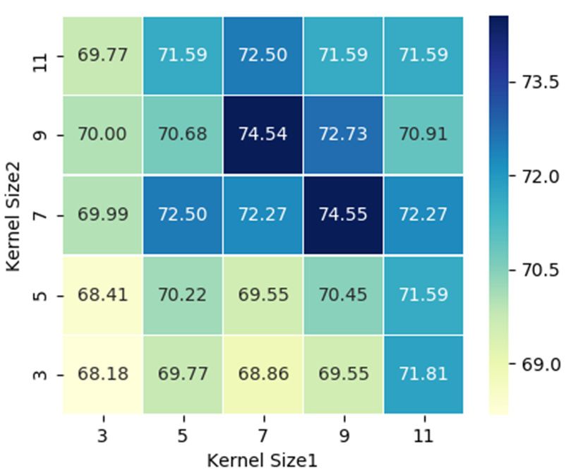
Scalestheof price trend in combination with multiple time scale features (
Features
F1 , F2 and F 3 ), we need to determine appropriate time scales for these features in order to predict
Considering that we predict the price trend in combination with multiple time scale features
(F1 , F2accurately.
more and F3 ), weSpecifically, since we
need to determine directly treat
appropriate timethe daily
scales fordata
theseasfeatures
the feature sequence
in order ( F1 more
to predict ), we
only need to
accurately. determinesince
Specifically, timewe scales for treat
directly features learned
the daily databyasCNN ( F2 and
the feature F 3 ). Time
sequence scales
(F1 ), we F2
onlyofneed
and
to F 3 correspond
determine time scalesto the receptivelearned
for features fields, by
which
CNNare(F2determined by kernel
and F3 ). Time scales of size
F2 and F stride of max-
3 correspond
to the receptive
pooling operationfields,
andwhich are determined
convolution operation. bySince
kernel
wesize
fix and
otherstride of max-pooling
parameters as common operation
values,andwe
convolution
only need tooperation.
adjust kernelSincesizes
we fix otherconvolution
of two parameters layers
as common
to findvalues,
morewe only needtime
appropriate to adjust kernel
scales. The
sizes
resultsof are
twoshown
convolution layers
in Figure to find5a,b
5. Figure more appropriate
represent time scales.
experimental The when
results resultspredicting
are shownprice in Figure
trends5.
Figure
one week 5a,band
represent experimental
one month results whenThe
later, respectively. predicting
abscissaprice trends the
represents one convolution
week and one month
kernel later,
size of
respectively.
the first layerThe abscissa
of CNN, whilerepresents the convolution
the ordinate kernel
represents the size of thekernel
convolution first layer
size ofof the
CNN, whilelayer
second the
ordinate
of CNN.represents
The largerthe theconvolution
convolutionkernel kernelsize of the
size, the second layer
larger the of CNN.
time scale of The larger the
features. The convolution
numerical
kernel
valuessize, the
in the largerrepresent
figure the time Accuracy
scale of features. The numerical
of the model values to
corresponding in the
the point.
figure represent Accuracy
of the model corresponding to the point.
(a) (b)
Figure 5.
Figure 5. The determination of time scales of features.
features. (a) Results for predicting the price trend
trend in
in one
one
week; (b)
week; (b) Results
Results for
for predicting
predictingthe
theprice
pricetrend
trendininone
onemonth.
month.
In
In Figure
Figure5,5,weweobserve
observe that when
that predicting
when the price
predicting trendtrend
the price one week later, the
one week convolution
later, kernel
the convolution
sizes
kernel ofsizes
two of
convolutional layers are
two convolutional preferably
layers 7 and 5,
are preferably respectively.
7 and Therefore,
5, respectively. the time
Therefore, thescales of F2
time scales
of FF23 are
and F3 are days
and8 trading and 18
8 trading trading
days and 18days, that is,
trading each
days, point
that in F2 point
is, each in F2 byisthe
is obtained closingby
obtained price
the
sequence of 8 trading days, and each
closing price sequence of 8 trading days, andpoint in F is obtained by the closing price sequence
3 each point in F 3 is obtained by the closing price of 18 trading
days. Similarly, when predicting the price trend
sequence of 18 trading days. Similarly, when predicting one month thelater,
pricethe sizesone
trend of two
monthconvolution
later, the kernels
sizes of
are preferably 9 and 7. In this case, the time scales of F 2 and F3 the time scales of F 24
are 10 trading days and tradingare days.
two convolution kernels are preferably 9 and 7. In this case, 2 and F 3 10
trading days and 24 trading days.
In addition, we can find that time scales of the features used to predict the price trend in a month
is larger than that used to predict the price trend in a week. This is consistent with our experience,
that is, larger-grained data are used for long-term forecasting, and smaller-grained data are used for
short-term forecasting.Appl. Sci. 2020, 10, 3961 10 of 14
Appl. Sci. 2020, 10, x FOR PEER REVIEW 10 of 15
In addition,
In this part, we
we can
investigate
find thatthe advantages
time of the
scales of the proposed
features used hybrid neural
to predict network
the price trendin in
combining
a month
multiple
is larger thantimethat
scaleused
features. We compared
to predict the price the
trendproposed network
in a week. with
This is models with
consistent basedour on experience,
single time
scaleis,features
that in accuracy.
larger-grained dataThe
are results
used forare reportedforecasting,
long-term in Table 1. The
andmodels F1 , are
based on data
smaller-grained F2 ,used F3
and for
represent the
short-term three models in Figure 3. They are all based on single time scale features.
forecasting.
4.2.2. Comparisons
Table 1.with Models Based
Comparisons on Single
with models Time
based Scaletime
on single Features
scale features in accuracy.
In this part, we investigate the advantages of the proposed hybrid neural network in combining
Forecast Horizon Model Accuracy (%)
multiple time scale features. We compared the proposed network with models based on single time
scale features in accuracy. The results are Model
reportedbased on F11. The models
in Table 64.40 based on F1 , F2 , and F3
represent the three models in Figure 3. They are all based on single time scale features.
Model based on F2 63.30
One week
Table 1. Comparisons with models based on single time scale features in accuracy.
Model based on F3 61.76
Forecast Horizon Model Accuracy (%)
The proposed model 66.59
Model based on F1 64.40
Model
Modelbased F2F1
basedonon 71.1463.30
One week
Model based on F3 61.76
The proposed
Model on F2
basedmodel 70.2366.59
One month Model based on F1 71.14
Modelbased
Model F2F3
basedonon 73.6470.23
One month
Model based on F3 73.64
The proposed model
The proposed model
74.5574.55
Table 1 shows that combining the features of multiple time scales can promote accurate
Table 1 shows that combining the features of multiple time scales can promote accurate prediction.
prediction. The models based on F1 , F2 , and F3 are based on the features of a single time scale,
The models based on F1 , F2 , and F3 are based on the features of a single time scale, while the proposed
while the proposed hybrid neural network
hybrid neural network combines the features of combines
multiplethe
timefeatures
scales toofpredict
multiple
thetime
trend.scales to predict
The predictive
the trend. The predictive performance of the hybrid neural network is better than
performance of the hybrid neural network is better than other networks. Therefore, combining the other networks.
Therefore,
features combining
of multiple thescales
time features of multiple time scales is helpful.
is helpful.
In the
In the next
next group
group of
of experiments,
experiments, taking
taking forecasting
forecasting price
price trends
trends one
one week
week later
later as
as an
an example,
example,
we visualize the trend prediction using test samples, as shown in Figures 6–8. From
we visualize the trend prediction using test samples, as shown in Figures 6–8. From these graphs, these graphs, we
cancan
we intuitively understand
intuitively understandthethe
benefits of combining
benefits of combiningfeatures of multiple
features of multipletime scales.
time scales.
Figure 6. Visualization of the trend prediction by different models on test example 1.
Figure 6. Visualization of the trend prediction by different models on test example 1.Appl. Sci. 2020, 10, x FOR PEER REVIEW 11 of 15
Appl. Sci. 2020, 10, 3961 11 of 14
Appl. Sci. 2020, 10, x FOR PEER REVIEW 11 of 15
Figure 7. Visualization of the trend prediction by different models on test example 2.
Figure 7. Visualization of the trend prediction by different models on test example 2.
Figure 7. Visualization of the trend prediction by different models on test example 2.
Figure 8. Visualization of the trend prediction by different models on test example 3.
Figure 8. Visualization of the trend prediction by different models on test example 3.
In Figure 6, we
Figure can find that
8. Visualization duetrend
of the to the influence
prediction of short-term
by different models fluctuations,
on test examplein3. some cases,
In Figure
the model based6,on
weF can find
fails to that due
predict thetoprice
the influence
trend in a of short-term
week fluctuations,
accurately. in Figure
Similarly, in some cases, the
7, Model
1
model
based based
Inon
Figureon F1 medium-term
6, we
F2 extracts failsfind
can to predict thetoprice
that due
features totrend
the in the
influence
predict a week
oftrend,accurately.
short-term Similarly,
fluctuations,
but ultimately in
fails in Figure
some
due 7,neglect
Model
cases,
to the the
based
model
of on F2on
based
long-term and Fshort-term
extracts
1
medium-term
fails to predict
changes features
thein
price to predict
trend
price in aIn
series. week theaccurately.
Figure trend,
8, thebut ultimately
Similarly,
model based inonfails
F3 due
Figure topays
the
7, Model
only
neglecton
based
attention ofto F2theextracts
long-term and
long-term short-term
medium-term changes
characteristics featuresin to
in the price series.
predict
price series In
theandFigure
trend,
cannot8, the
but model based
ultimately
accurately failson
predict due F 3to
the only
the
trend.
Therefore,
pays attention
neglect we can to conclude
of long-term theand that predicting
long-term
short-term changes theinprice
characteristics trend
in the
price based
price
series. In on features
series and
Figure theof
8, cannot a single time
accurately
model based scale
F 3 isonly
onpredict not
the
feasible
pays in some
trend.attention
Therefore, cases
we can
to the due to the
conclude
long-term complexity and
that predicting
characteristics variability
theprice
in the of
priceseriesprice
trend andseries.
based It makes
on features
cannot sense to combine
of a predict
accurately single timethe
the
scalefeatures
is not of multiple
feasible in time
some scales
cases to
due predict
to the the future
complexity price
and trend.
variability of price
trend. Therefore, we can conclude that predicting the price trend based on features of a single time series. It makes sense
to combine
scale the features
is not feasible in someof multiple
cases due time scales
to the to predict
complexity andthevariability
future price trend.series. It makes sense
of price
4.2.3. Comparisons with Existing Models
to combine the features of multiple time scales to predict the future price trend.
4.2.3.Due
Comparisons with Existing
to the differences in dataModels
preprocessing, model training methods, and learning targets, it is
4.2.3.easy
not Comparisons
Due totodirectly with
the differences Existing
compare dataModels
inamong existing works,
preprocessing, we try
model to select
training some and
methods, models commonly
learning targets,usedit is
in financial
not easy forecasting and adjust these models to the best state to make relatively fair comparisons.
Due to the differences in data preprocessing, model training methods, and learning targets, it in
to directly compare among existing works, we try to select some models commonly used is
The experimental
financial forecasting results
andare shown
adjust thesein Table
models 2. to the best state to make relatively fair comparisons.
not easy to directly compare among existing works, we try to select some models commonly used in
The experimental
financial forecasting results
and areadjustshown
these inmodels
Table 2.to the best state to make relatively fair comparisons.
The experimental results are shown in Table 2.
Table 2. Comparisons with existing models in accuracy.
Table 2. Comparisons with existing models in accuracy.
Forecast Horizon Model Accuracy (%)
Forecast Horizon Model Accuracy (%)Appl. Sci. 2020, 10, 3961 12 of 14
Table 2. Comparisons with existing models in accuracy.
Forecast Horizon Model Accuracy (%)
Simplistic Model 54.82
SVM 61.98
LSTM 65.05
One week CNN 59.34
Multiple Pipeline Model 63.30
NFNN 65.93
The proposed model 66.59
Simplistic Model 56.92
SVM 70.91
LSTM 71.59
One month CNN 67.95
Multiple Pipeline Model 72.05
MFNN 72.27
The proposed model 74.55
From Table 2, we can find that the proposed hybrid neural network performs better than other
models, whether the forecast horizon is one week or one month. On the one hand, SVM is a commonly
used machine learning model in financial forecasting, while CNN and LSTM are commonly used deep
learning models. Compared with the Simplistic Model, these models can extract profitable information,
but they only learn features from a single scale and ignore some useful information. On the other hand,
the Multiple Pipeline Model and MFNN are models based on multi-scale feature learning for financial
time series forecasting. They use different branches or different networks to extract different scale
features. However, it will increase the complexity of the model. The model we proposed only utilizes
a CNN to extract features of different scales simplifying the model and predicting more accurately.
Therefore, we can conclude that the proposed hybrid neural network is superior to the commonly used
models in the existing works.
5. Discussion
In this paper, we propose a hybrid neural network based on multiple time scale feature learning
for stock market index trend prediction. Because there are multi-scale features in financial time series,
it makes sense to combine them to predict future trends. First, the proposed model only utilizes one
CNN to extract multiple time scale features, instead of using multiple networks like other models.
It simplifies the model and makes more accurate predictions. Second, time dependences in the multiple
time scale features are learned by three LSTMs. Finally, the information learned by LSTMs is fused
through fully connected layers to predict the price trend.
The experimental results demonstrate that such a hybrid network can indeed enhance the
predictive performance compared with benchmark networks. Firstly, by comparing with the models
based on F1 , F2 and F3 , we conclude that combining multiple time scale features can promote accurate
prediction. Secondly, in comparison with the Simplistic Model, we found that the proposed model
can learn valuable information. SVM, CNN, and LSTM all learn the features in price series from a
single scale. However, there are multiple scales in financial time series, which makes these methods
sometimes unable to perform accurate predictions. Finally, both the Multiple Pipeline Model and
MFNN are models based on multi-scale feature learning, but they use several branches or networks
to extract multi-scale features, making the network huge and complex. The hybrid neural network
we proposed uses only a CNN to extract multi-scale features, simplifying the model and predicting
more accurately.
However, we can find that the proposed model cannot accurately predict trends for some data
samples. There may be two reasons for this issue. First, the three time scales features are not enough to
reflect the internal law of price series. Second, these samples are seriously affected by other factors thatAppl. Sci. 2020, 10, 3961 13 of 14
we have not considered, such as political policy, industrial development, natural factors, and so on.
It provides directions for our future work. We can consider using a multi-layer CNN to extract more
scale features for prediction. At the same time, we can extract useful information from more sources,
such as macroeconomic indicators, news, market sentiment and so on.
Author Contributions: Y.H. proposed the basic framework of hybrid neural network and completed the model
construction, experimental research, and thesis writing. Throughout the process, Q.G. guided and gave a lot of
suggestions. All authors have read and agreed to the published version of the manuscript.
Funding: This research received no external funding.
Conflicts of Interest: The authors declare no conflict of interest.
References
1. Qiu, M.; Song, Y. Predicting the Direction of Stock Market Index Movement Using an Optimized Artificial
Neural Network Model. PLoS ONE 2016, 11, e0155133. [CrossRef] [PubMed]
2. Adebiyi, A.; Adewumi, A.; Ayo, C.K. Comparison of ARIMA and Artificial Neural Networks Models for
Stock Price Prediction. J. Appl. Math. 2014, 2014, 1–7. [CrossRef]
3. Pai, P.-F.; Lin, C.-S. A hybrid ARIMA and support vector machines model in stock price forecasting. Omega
2005, 33, 497–505. [CrossRef]
4. Kara, Y.; Acar, M.; Baykan, Ö.K. Predicting direction of stock price index movement using artificial neural
networks and support vector machines: The sample of the Istanbul Stock Exchange. Expert Syst. Appl. 2011,
38, 5311–5319. [CrossRef]
5. Di Persio, L.; Honchar, O. Artificial neural networks architectures for stock price prediction: Comparisons
and applications. Int. J. Circuits Syst. Signal Process. 2016, 10, 403–413.
6. Masoud, N. Predicting Direction of Stock Prices Index Movement Using Artificial Neural Networks: The Case
of Libyan Financial Market. Br. J. Econ. Manag. Trade 2014, 4, 597–619. [CrossRef]
7. Inthachot, M.; Boonjing, V.; Intakosum, S. Artificial Neural Network and Genetic Algorithm Hybrid
Intelligence for Predicting Thai Stock Price Index Trend. Comput. Intell. Neurosci. 2016, 2016, 1–8. [CrossRef]
[PubMed]
8. Qiu, M.; Song, Y.; Akagi, F. Application of artificial neural network for the prediction of stock market returns:
The case of the Japanese stock market. Chaos Solitons Fractals 2016, 85, 1–7. [CrossRef]
9. Chong, E.; Han, C.; Park, F.C. Deep learning networks for stock market analysis and prediction: Methodology,
data representations, and case studies. Expert Syst. Appl. 2017, 83, 187–205. [CrossRef]
10. Singh, R.; Srivastava, S. Stock prediction using deep learning. Multimedia Tools Appl. 2016, 76, 18569–18584.
[CrossRef]
11. Fischer, T.; Krauss, C. Deep learning with long short-term memory networks for financial market predictions.
Eur. J. Oper. Res. 2018, 270, 654–669. [CrossRef]
12. Si, W.; Li, J.; Ding, P.; Rao, R. A Multi-objective Deep Reinforcement Learning Approach for Stock Index
Future’s Intraday Trading. In Proceedings of the 2017 10th International Symposium on Computational
Intelligence and Design (ISCID), Hangzhou, China, 9–10 December 2017; IEEE: New York, NY, USA, 2017;
pp. 431–436.
13. Bao, W.; Yue, J.; Rao, Y. A deep learning framework for financial time series using stacked autoencoders and
long-short term memory. PLoS ONE 2017, 12, e0180944. [CrossRef] [PubMed]
14. Sirignano, J.; Cont, R. Universal features of price formation in financial markets: perspectives from deep
learning. Quant. Financ. 2019, 19, 1449–1459. [CrossRef]
15. Tsantekidis, A.; Passalis, N.; Tefas, A.; Kanniainen, J.; Gabbouj, M.; Iosifidis, A. Using deep learning to detect
price change indications in financial markets. In Proceedings of the 2017 25th European Signal Processing
Conference (EUSIPCO), Kos, Greek, 28 August–2 September 2017; Institute of Electrical and Electronics
Engineers (IEEE): New York, NY, USA, 2017; pp. 2511–2515.
16. Chen, C.-T.; Chen, A.-P.; Huang, S.-H. Cloning Strategies from Trading Records using Agent-based
Reinforcement Learning Algorithm. In Proceedings of the 2018 IEEE International Conference on Agents
(ICA), Singapore, 28–31 July 2018; Institute of Electrical and Electronics Engineers (IEEE): New York, NY,
USA, 2018; pp. 34–37.Appl. Sci. 2020, 10, 3961 14 of 14
17. Siripurapu, A. Convolutional Networks for Stock Trading; Stanford University Department of Computer Science:
Stanford, CA, USA, 2014.
18. Gunduz, H.; Yaslan, Y.; Cataltepe, Z. Intraday prediction of Borsa Istanbul using convolutional neural
networks and feature correlations. Knowl.-Based Syst. 2017, 137, 138–148. [CrossRef]
19. Liu, S.; Zhang, C.; Ma, J. CNN-LSTM Neural Network Model for Quantitative Strategy Analysis in Stock
Markets. In Proceedings of the International Conference on Neural Information Processing, Guangzhou,
China, 14–18 November 2017; Springer: Cham, Switzerland, 2017; pp. 198–206.
20. Wang, Y.; Zhang, C.; Wang, S.; Yu, P.S.; Bai, L.; Cui, L. Deep Co-Investment Network Learning for Financial
Assets. In Proceedings of the 2018 IEEE International Conference on Big Knowledge (ICBK), Singapore,
17–18 November 2018; Institute of Electrical and Electronics Engineers (IEEE): New York, NY, USA, 2018;
pp. 41–48.
21. Eapen, J.; Bein, D.; Verma, A. Novel Deep Learning Model with CNN and Bi-Directional LSTM for Improved
Stock Market Index Prediction. In Proceedings of the 2019 IEEE 9th Annual Computing and Communication
Workshop and Conference (CCWC), Las Vegas, NV, USA, 7–9 January 2019; Institute of Electrical and
Electronics Engineers (IEEE): New York, NY, USA, 2019; pp. 0264–0270.
22. Long, W.; Lu, Z.; Cui, L. Deep learning-based feature engineering for stock price movement prediction.
Knowl.-Based Syst. 2019, 164, 163–173. [CrossRef]
23. Luo, W.; Li, Y.; Urtasun, R.; Zemel, R. Understanding the effective receptive field in deep convolutional
neural networks. In Advances in Neural Information Processing Systems, Barcelona, SPAIN, 5–10 December 2016;
MIT Press: Cambridge, MA, USA, 2016; pp. 4898–4906.
24. Hochreiter, S.; Schmidhuber, J. Long Short-Term Memory. Neural Comput. 1997, 9, 1735–1780. [CrossRef]
[PubMed]
25. Chung, J.; Gulcehre, C.; Cho, K.H.; Bengio, Y. Empirical evaluation of gated recurrent neural networks on
sequence modeling. arXiv 2014, arXiv:1412.3555.
26. Krizhevsky, A.; Sutskever, I.; Hinton, G.E. Imagenet classification with deep convolutional neural networks.
In Advances in Neural Information Processing Systems; MIT Press: Cambridge, MA, USA, 2012; pp. 1097–1105.
27. Jaitly, N.; Zhang, Y.; Chan, W. Very Deep Convolutional Neural Networks for End-To-End Speech Recognition.
U.S. Patent No 10,510,004, 1 August 2019.
28. I Widiastuti, N. Convolution Neural Network for Text Mining and Natural Language Processing.
In Proceedings of the IOP Conference Series: Materials Science and Engineering, Bandung, Indonesia,
18 July 2019; IOP Publishing: Bristol, UK, 2019; Volume 662, p. 052010.
29. Yahoo Finance, S & P 500 Stock Data. Available online: https://finance.yahoo.com/quote/%5EGSPC/history?
p=%5EGSPC (accessed on 1 February 2019).
30. Andrychowicz, M.; Denil, M.; Gomez, S.; Hoffman, M.W.; Pfau, D.; Schaul, T.; Shillingford, B.; De Freitas, N.
Learning to learn by gradient descent by gradient descent. In Advances in Neural Information Processing
Systems; MIT Press: Cambridge, MA, USA, 2016; pp. 3981–3989.
31. Srivastava, N.; Hinton, G.; Krizhevsky, A.; Sutskever, I.; Salakhutdinov, R. Dropout: A simple way to prevent
neural networks from overfitting. J. Mach. Learn. Res. 2014, 15, 1929–1958.
32. Ioffe, S.; Szegedy, C. Batch normalization: Accelerating deep network training by reducing internal covariate
shift. arXiv 2015, arXiv:1502.03167.
© 2020 by the authors. Licensee MDPI, Basel, Switzerland. This article is an open access
article distributed under the terms and conditions of the Creative Commons Attribution
(CC BY) license (http://creativecommons.org/licenses/by/4.0/).You can also read


