Site and Regional Trend Analysis of Precipitation in Central Macedonia, Greece
←
→
Page content transcription
If your browser does not render page correctly, please read the page content below
Computational Water, Energy, and Environmental Engineering, 2021, 10, 49-70
                                                                                               https://www.scirp.org/journal/cweee
                                                                                                            ISSN Online: 2168-1570
                                                                                                              ISSN Print: 2168-1562

Site and Regional Trend Analysis of
Precipitation in Central Macedonia, Greece

Athanasios K. Margaritidis

Faculty of Agriculture, Forestry and Natural Environment, School of Agriculture, Department of Hydraulics,
Soil Science & Agriculture Engineering, Thessaloniki, Greece

How to cite this paper: Margaritidis, A.K.      Abstract
(2021) Site and Regional Trend Analysis of
Precipitation in Central Macedonia, Greece.     The purpose of this paper is to investigate the trend of precipitation in Kilkis
Computational Water, Energy, and Envi-          region (Greece) at the site and regional level in various time scales. At the site
ronmental Engineering, 10, 49-70.
                                                level, the precipitation trend was analyzed using three tests: 1) Mann-Kendall,
https://doi.org/10.4236/cweee.2021.102004
                                                2) Sen’s T and 3) Spearman while the trend slope was estimated using the
Received: January 16, 2021                      Sen’s estimator. At a regional level, nonparametric spatial tests such as Re-
Accepted: April 13, 2021                        gional Average Mann-Kendall (RAMK) and BECD’s (Bootstrap Empirical
Published: April 16, 2021
                                                Cumulative Distributions) were elaborated with and without the effect of
Copyright © 2021 by author(s) and               cross correlation. The trend of precipitation was noticed generally downward
Scientific Research Publishing Inc.             at annual time scale and statistically significant at 5% level of significance on-
This work is licensed under the Creative
                                                ly in only one station. The results of the analysis of trends at the regional level
Commons Attribution International
License (CC BY 4.0).                            showed in total the influence of cross correlation in the time series since the
http://creativecommons.org/licenses/by/4.0/     number of trends detected is reduced when cross correlation is preserved.
                Open Access                     Precipitation data from 12 stations were used. The study results benefit water
                                                resource management, drought mitigation, socio-economic development, and
                                                sustainable agricultural planning in the region.

                                                Keywords
                                                Sen’s T Test, Bootstrap Test, Precipitation, Trend Analysis, Greece

                                              1. Introduction
                                              As global climate change may affect long-term precipitation patterns resulting in
                                              an increase in droughts and floods, the continuous variability of precipitation
                                              around the world deserves urgent attention [1]. According to Climate Change
                                              2007 [2] for a future warmer climate, the current generation of models shows
                                              that maximum precipitation generally increases in tropical areas (monsoon re-
                                              gimes) and over the tropical Pacific, with general decreases in the subtropics and

DOI: 10.4236/cweee.2021.102004          Apr. 16, 2021               49     Computational Water, Energy, and Environmental Engineering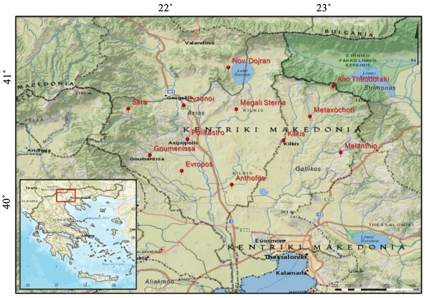
A. K. Margaritidis

                                 increases in high latitudes, hampering the general intensification of the global
                                 hydrological cycle. The average of water vapor, evaporation and precipitation
                                 worldwide, is expected to increase. However, for example in China while an an-
                                 nual upward trend is observed, significant seasonal variations occur in several
                                 regions [3] [4]. Furthermore [5], point out the necessity to pay more attention to
                                 the prevention and mitigation of drought events that may occur in spring and
                                 summer periods. The results of the trend of precipitation in spatial levels of cli-
                                 matic regions of Canada [6] seem to be respective with emergence of an upward
                                 trend in the average precipitation in the northern region and a downward trend
                                 in the south-west, statistically significant at 5% significance level.
                                   In Europe, and especially in the Mediterranean area recent researches [7]-[14]
                                 have shown a reduction of annual precipitation. Precipitation levels in Greece
                                 fluctuate extremely abnormally, both spatially and temporally resulting in an
                                 uneven distribution of water resources availability. More specifically, the pattern
                                 of precipitation indicates severe changes between the western part of Greece
                                 (greater precipitation level) and the other regions of the country. Several studies
                                 concerning precipitation variability [15] [16] [17] [18] [19], for a large number
                                 of meteorological stations in Greece show a downward trend which in some
                                 areas appears to be statistically significant.
                                   The aim of this paper is to study the variation of precipitation and trend anal-
                                 ysis with non-parametric methods in both site and spatial level for various time
                                 scales using 12 rain stations distributed as uniformly as possible in the geo-
                                 graphical wider area of Kilkis region (Greece). An additional goal of this study is
                                 to investigate whether the drop of Lake Doirani from 146.3 meters to 141.1 me-
                                 ters in 2002 [19], is due to a statistically significant drop in precipitation at sta-
                                 tion level (Nov. Dojran) or area or exogenous factors. It is also worth mention-
                                 ing that the investigation of trends in the study area has not been the subject of
                                 research for this period (1973-2008) with so many stations and so many periods,
                                 while special reference should be made to the fact that from 2011 onwards, most
                                 of the rain gauges have stopped working. The precipitation is recorded by the
                                 automatic meteorological station in the area of Kilkis (2004-present) and by the
                                 corresponding one in the area of Doirani in the Greek territory. Since precipita-
                                 tion is the main component of agricultural water management in the study area,
                                 a better understanding of its behavior through trend analysis can contribute sig-
                                 nificantly to the estimation of water resource availability and the development of
                                 adequate irrigation practices and crop patterns.

                                 2. Materials and Methods
                                 2.1. Study Area
                                 The study area is situated in Northern Greece including the Prefecture of Kilkis
                                 bordering in the north with F.Y.R.O.M. (Figure 1). The climate of the study area
                                 is characterized as dry and warm (semi-arid) with moderate annual precipita-
                                 tion. From a geomorphological point of view, the terrain of the Prefecture of

DOI: 10.4236/cweee.2021.102004                          50     Computational Water, Energy, and Environmental Engineering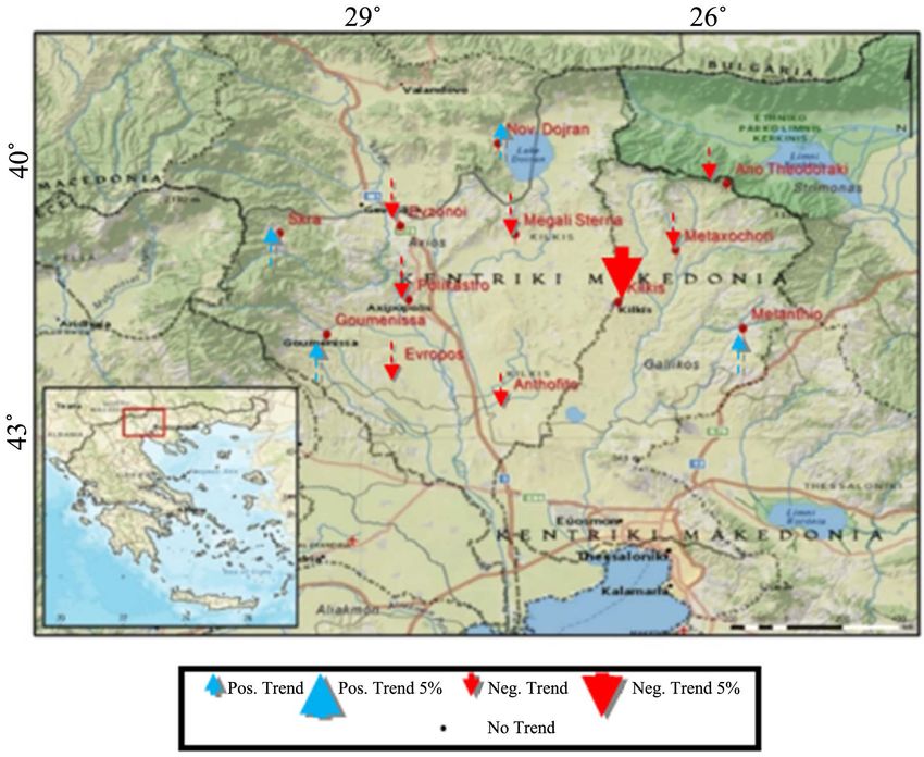
A. K. Margaritidis

                                 Figure 1. Study area, water basins and the distribution of selected stations (Basemap: Esri
                                 & Open Street Map).

                                 Kilkis is determined by the morphological characteristics of different hydrologi-
                                 cal basins (Figure 1). The basins, in which the study area is divided, are the ba-
                                 sin of Lake Doiran (only part of the basin from the side of Greece), the Gallikos
                                 river basin, the basin of the Axios River and finally the Strimonas River basin (a
                                 part of Prefecture of Kilkis).

                                 2.2. Data
                                 The precipitation data used in this analysis were taken by 12 meteorological sta-
                                 tions of the study area and cover the period 1973-2008 (36 years) (Table 1). In
                                 addition, these stations, at least in the Greek side, were consisted of pluviometers
                                 and rain gauges. As it can be noticed from Figure 1 and Table 1, the meteoro-
                                 logical stations Ano Theodoraki, Metaxochori, Kilkis and Melanthio are located
                                 in the basin of the Gallikos river basin, the stations Evzonoi, Megali Sterna,
                                 Goumenissa, Polikastro, Skra, Evropos and Anthofito in the basin of the Axios
                                 River while the station Nov. Dojran (F.Y.R.O.M.) in the basin of Lake Doiran.
                                   A preliminary examination of monthly values showed that the data of stations
                                 contain very little measurement gaps. Specifically, in the time series Nov. Dojran
                                 two missing values appeared in 2001 during the months of January and Febru-
                                 ary, one value in the year 2007 in the same time series in July and one more in
                                 August 2008, which consist an almost zero percentage of the total value range
                                 (0.08%).
                                   In this paper, in order to fill in the time series, the weather station Polikastro
                                 was defined as a reference station, to fill in the missing values of the meteoro-
                                 logical station Nov. Dojran. The reasons for this choice, are related to the relia-
                                 bility of the data (it is placed on the same altitude, it is located spatially closer to

DOI: 10.4236/cweee.2021.102004                          51        Computational Water, Energy, and Environmental Engineering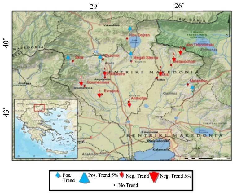
A. K. Margaritidis

                                 Table 1. Water basins, elevation above the sea level and mean annual precipitation (mm)
                                 for the stations of study area.

                                           Station     Hydrological Basin     Elevation (m)   Mean Annual Precipitation (mm)

                                         Nov. Dojran      Doiran Lake              141                    632.2

                                    Ano Theodoraki       Gallikos River            480                    433.6

                                         Metaxochori     Gallikos River            277                    521.6

                                            Kilkis       Gallikos River            275                    441.7

                                          Melanthio      Gallikos River            490                    587.6

                                          Anthofito       Axios River               60                    514.6

                                     Megali Sterna        Axios River              125                    541.3

                                          Evzonoi         Axios River               90                    566.2

                                          Polikastro      Axios River               50                    589.8

                                          Evropos         Axios River               70                    488.0

                                         Goumenissa       Axios River              260                    719.2

                                            Skra          Axios River              540                    736.8

                                 the Melanthio station) as well as with the better links between them (cross-cor-
                                 relation) of time series (Table 2). The method of filling gaps was the linear re-
                                 gression sum to zero (negative values) with the introduction of a random term
                                 [20].

                                 2.3. Methods
                                 After the successful analysis of the homogeneity [21], of the time series, an explo-
                                 ration of trends in precipitation is elaborated at site level using Mann-Kendall,
                                 Sen’s T test, Sen’s estimate of slope and Spearman and at regional level using Re-
                                 gional Average Mann-Kendall and Bootstrap tests (5% significance level) in vari-
                                 ous time scales (Figure 2).
                                   Lag-1 Serial Correlation (pre-whitening)
                                   The approach of pre-whitening is one of the most common methods for cal-
                                 culating the serial correlation and its removal from the examined time series on
                                 condition that the calculated serial correlation is statistically significant at 5%
                                 level of significance (Table 3). The pre-whitening is performed as follows [22]:
                                                                     X t′= xt +1 − r1 ⋅ xt                               (1)

                                 where X t′ is the pre-whitened time series for time interval t, xt and xt+1 the ini-
                                 tial time series for the time interval t and t + 1 respectively while r1 is the lag-1
                                 autocorrelation coefficient.
                                   Mann-Kendall test
                                   It consists one of the main and most widespread test non-parametric statistic-
                                 al tests in hydrometeorology. According to this test the null hypothesis Ho and
                                 the alternative H1 are defined as follows:
                                   Ho: Observations with no monotonic trend

DOI: 10.4236/cweee.2021.102004                          52      Computational Water, Energy, and Environmental Engineering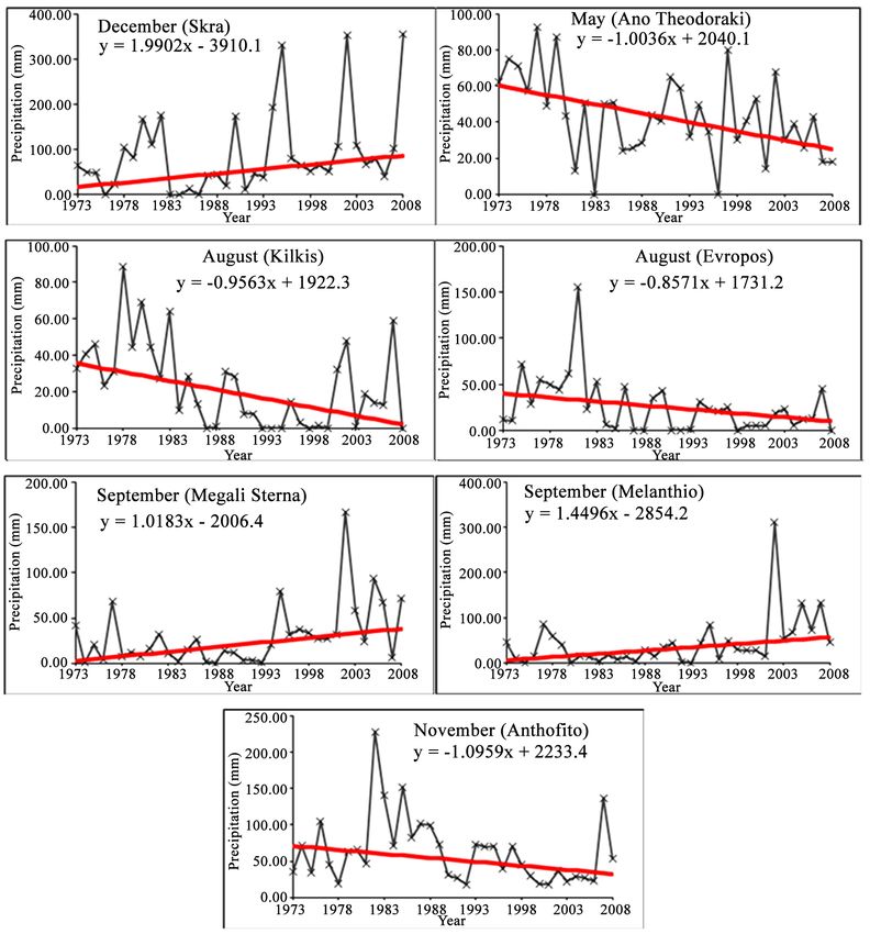
A. K. Margaritidis

Table 2. Cross-correlation coefficients between stations.

    Station (*)          1.         2.         3.          4.         5.           6.          7.            8.        9.           10.             11.       12.
         1.              1        0.462       0.493      0.393      0.667         0.237       0.540         0.407    0.576         0.483           0.427     0.423
         2.            0.462         1        0.505      0.304      0.535         0.249       0.630         0.103    0.454         0.543           0.363     0.433
         3.            0.493      0.505         1        0.639      0.570         0.388       0.419         0.122    0.457         0.496           0.356     0.412
         4.            0.393      0.304       0.639        1        0.526         0.404       0.322         0.324    0.395         0.502           0.276     0.411
         5.            0.667      0.535       0.570      0.526        1           0.212       0.565         0.461    0.624         0.540           0.346     0.538
         6.            0.237      0.249       0.388      0.404      0.212            1        0.349         0.397    0.202         0.490           0.482     0.547
         7.            0.540      0.630       0.419      0.322      0.565         0.349        1            0.274    0.659         0.700           0.509     0.538
         8.            0.407      0.103       0.122      0.324      0.461         0.397       0.274          1       0.367         0.450           0.334     0.680
         9.            0.576      0.454       0.457      0.395      0.624         0.202       0.659         0.367      1           0.505           0.422     0.521
        10.            0.483      0.543       0.496      0.502      0.540         0.490       0.700         0.450    0.505           1             0.590     0.622
        11.            0.427      0.363       0.356      0.276      0.346         0.482       0.509         0.334    0.422         0.590             1       0.600
        12.            0.423      0.433       0.412      0.411      0.538         0.547       0.538         0.680    0.521         0.622           0.600       1

*1. Nov. Dojran, 2. Ano Theodoraki, 3. Metaxochori, 4. Kilkis, 5. Melanthio, 6. Anthofito, 7. Megali Sterna, 8. Evzonoi, 9. Polikastro, 10. Evropos, 11. Gou-
menissa, 12. Skra.

                                                Table 3. Time series with serial correlation at first lag, serial correlation levels at 5% level
                                                of significance and serial correlation values in all time periods of the study.

                                                       Period          Lower bound           Upper bound            Stations with Lag-1 Serial Correlation
                                                       Annual               −0.314                  0.314                   0.5654, 0.5645, 0.4078, 0.3779
                                                      Irrigation            −0.314                  0.314                          0.3214, 0.3935
                                                       Spring               −0.314                  0.314                             −0.33011
                                                      Autumn                −0.314                  0.314                          0.3684, 0.3418
                                                                                                      Months
                                                      October               −0.314                  0.314                                 0.3237
                                                      December              −0.314                  0.314                                 0.3585
                                                       January              −0.314                  0.314                0.3726, 0.3837, 0.42810, 0.36711
                                                       March                −0.314                  0.314                                 0.3336
                                                         May                −0.314                  0.314                             −0.32811
                                                       August               −0.314                  0.314                                 0.3554

                                                1. Nov. Dojran. 2. Ano Theodoraki. 3. Metaxochori. 4. Kilkis. 5. Melanthio. 6. Anthofito. 7. Μegali Sterna.
                                                8. Εvzonoi. 9. Polikastro. 10. Evropos. 11. Goumenissa. 12. Skra.

                                                    Figure 2. Trend analysis procedures—study methodology.

DOI: 10.4236/cweee.2021.102004                                               53           Computational Water, Energy, and Environmental Engineering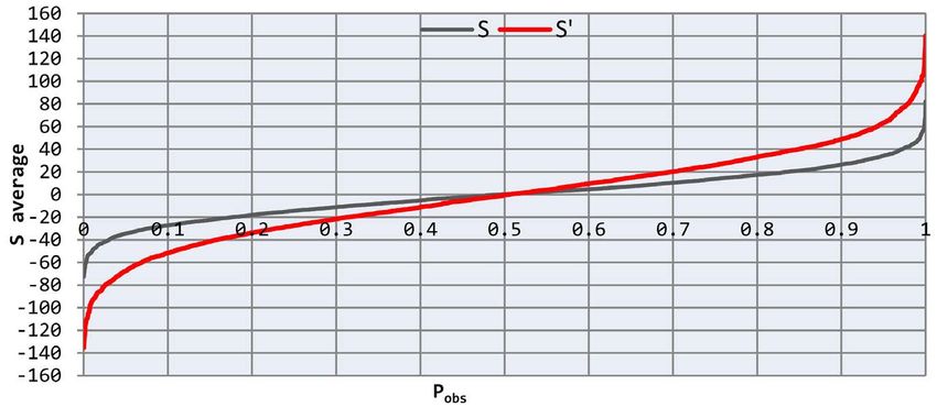
A. K. Margaritidis
H1: Observations with monotonic trend (upward or downward)
The M-K statistic S is calculated as follows [23] [24]:
n −1
sgn ( x j − xk )
n
=S ∑∑ (2)
k= 1 j= k +1
1 if ( x j − xk ) > 0
sgn ( x=
j − xk ) 0 if ( x= j − xk ) 0 (3)
−1 if ( x j − xk ) < 0
with xj and xk observations representing annual observations prices and k, j ≤ n
and k # j.
The variance of S is calculated by the following formula:
1
=
var S n ( n − 1)( 2n + 5 ) − ∑ t t ( t − 1)( 2t + 5 ) (4)
18
where the notation t refers to the extent of any given tie and ∑t states the
summation over all ties.
Using the value of S, the standard normal test statistic Z is computed:
S −1
var S if S > 0
=Z = 0 if S 0 (5)
S +1
if S < 0
var S
In two-sided statistical test for the presence of a trend, the null hypothesis Ho
should be accepted if Z ≤ Z α at a predefined significance level α (e.g. Z ≤
1−
2
1.96 at 95% confidence interval).
Sen’s-T test
It is classification method (ranked), which removes the seasonality from each
time series summarizing the data at different seasons in order to produce a sta-
tistical trend value [25] [26]. This process is distributed free and it is not affected
by seasonal variations [27]. The computational steps are:
The average for the month j is computed for a number of years n:
xij
X j = ∑ i =1 (6)
n
n
and the average for the year i
xij
X i = ∑ j =1
12
(7)
12
Then the average of each month is subtracted from each of the correspond-
ing months in the n years in order to remove seasonal effects e.g. Xij − Xj for
i = 1, 2, , n and j = 1, 2, ,12 .
The above differences (Xij − Xj) from 1 to n × m (n = number of years, m =
number of months) are ranked and a new table (Rij) is obtained, where Rij is
the rank of Xij − Xj.
DOI: 10.4236/cweee.2021.102004 54 Computational Water, Energy, and Environmental Engineering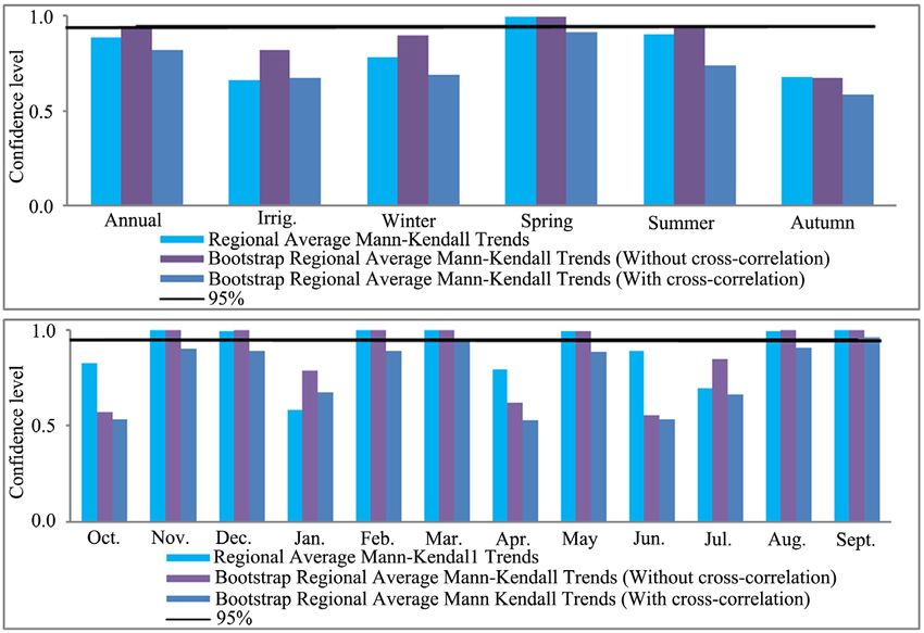
A. K. Margaritidis
The test statistic T is calculated by the following equation:
12m 2 n n +1 nm + 1
=T ∑ i =1 i − 2 Ri − 2 (8)
n ( n + 1) ∑ i , j ( Rij − R j )
2
For sample size (n), the trend Τ tends towards that of the standard normal
distribution under the null hypothesis of non-existence of trend. The Sen’s T test
statistic is compared to the standard normal variate Z in order to detect the
trend existence.
Sen’s Estimator of Slope
The Sen’s estimator is used in those cases that can be detected the presence of
a linear trend [17].
The estimate of the slope of the trend results from the median of the N slopes
Qi of data pairs:
x j − xk
Qi = (9)
j−k
when j > k , i = 1, 2, , N .
The estimate of the slope of the trend of Sen is the median of Qi ranked
from smallest to largest:
Q N +1 for odd values of N
2
Q = QN + QN + 2 (10)
2 2
for even values of N
2
Regional Average Mann-Kendall (RAMK) test
In the case of spatial data observation, i.e. split into (m) locations, test is ap-
plied to the data of each location, separating them essentially in (m) sub-series,
each of which represents a corresponding region [28] [29] [30]:
1 m
Sr = ∑ SL
m L =1
(11)
where Sr is the regional average M-K statistic and S L is the M-K statistic for
each L station in the region.
The variance of Sr is calculated by the following formula:
var=
Sr( ) 1
n ( n − 1)( 2n + 5 ) − ∑ t t ( t − 1)( 2t + 5 )
18m
(12)
where the notation t refers to the extent of any given tie and ∑t states the
summation over all ties.
The standard normal variate is computed as follows:
Sr
Zm = (13)
var Sr ( )
m
The statistical significance of Z m is computed from the Cumulative Distri-
DOI: 10.4236/cweee.2021.102004 55 Computational Water, Energy, and Environmental Engineering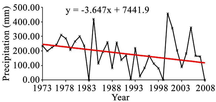
A. K. Margaritidis
bution Function of the standard normal variate.
Regional Average Mann-Kendall Bootstrap (RAMK-B) test
To find a general pattern of changes over a specific region, it is necessary to
assess the field significance of trends in the region. Like the existence of serial
correlation in time series, the presence of positive cross-correlation among sites
in a region will result in an increased probability of rejecting the null hypothesis
of no trend, while it might be actually true in some cases [28].
This study adopts a bootstrapping approach [30] [31] [32] that is similar in
spirit to the method [28]. The approach is described as follows:
1) The selected calculation period or range of years, for example, [1973,
1974, …, 2008] is resampled randomly with replacement. Then we can get a new
set with different year order from the original one but with the same length, for
instance, [1975, 1979, 1995, 1995, 2008].
2) Each site within a network has an observation value corresponding to a ca-
lendar year. By rearranging the observation values of each site of the network
according to the new year set obtained in step (1), a new network can be ob-
tained.
3) The M-K statistic (Equation (2)) at site L in the bootstrapped network can
be computed. The RAMK statistic can be calculated by equation (11).
4) By repeating steps (1)-(3) N times (i.e. N = 4000), N values of the RAMK
statistics can be obtained. Then the Bootstrap Empirical Cumulative Distribu-
tion (B.E.C.D.) of the RAMK statistic ( Sr ) can be obtained by ranking the N
values of the RAMK statistic in ascending order and assigning a non-exceedance
probability using the Weibull plotting position formula as:
r
P= (14)
N +1
where r is the rank of Sr in the bootstrap sample data according to the as-
cending order.
The probability value ( Pobs ) of the historical RAMK statistic can be obtained
by comparing it with the bootstrap empirical cumulative distributions. The cor-
responding Pf value is given by:
Pobs for Pobs ≤ 0.50
Pf = (15)
1 − Pobs for Pobs > 0.50
The field significance is obtained as follows: if Pf is less than α (level of signi-
ficance) then the trend is considered as field significant at the predefined α level
(1 − α confidence level).
In the above procedure, if one directly resamples the sample data at a site ra-
ther than the year series as in steps (1) and (2), then a BECD without preserving
cross-correlation structure of a network can be obtained.
3. Results
3.1. Site Trend Analysis
The precipitation data in all periods of study, for the 36 years, for the 12 stations
DOI: 10.4236/cweee.2021.102004 56 Computational Water, Energy, and Environmental EngineeringA. K. Margaritidis
of the study area, were investigated at site level.
In the annual observations, a statistically significant trend at a level of signifi-
cant 5% by all trend tests, appeared only in Kilkis station, as depicted both in
Figure 3 and in Table 4. Generally, for the whole study area, four stations had
positive trends while the remaining eight negative ones but only one station
showed a statistically significant downward trend in precipitation. Furthermore,
in all cases (Table 5(a) and Table 5(b)), the results of Mann-Kendall [33] and
Sen’s T tests were successfully verified by Spearman’s method.
Figure 3. Annual trend results with non-parametric test Mann-Kendall at 12 stations in
the study area.
Table 4. Trend results and slope estimation in the study area for annual time period.
Μ-Κ Sen’s Spearman
Station Sen-T
Test Z slope (mm/year) p value
Nov. Dojran 0.59 0.769 1.306 0.450
Ano Theodoraki −0.63 −0.628 −1.351 0.536
Metaxochori −1.21 −1.070 −3.344 0.290
Kilkis −1.99* −2.012* −3.647* 0.043*
Melanthio 0.27 0.362 0.572 0.724
Anthofito −0.83 −1.002 −2.316 0.322
Megali Sterna −0.37 −0.396 −0.993 0.697
Evzonoi −0.07 0.006 −0.431 0.995
Polikastro −0.76 −0.799 −3.139 0.430
Evropos −1.24 −1.332 −2.534 0.186
Goumenissa 0.45 0.387 1.477 0.703
Skra 0.31 0.519 1.370 0.609
DOI: 10.4236/cweee.2021.102004 57 Computational Water, Energy, and Environmental EngineeringA. K. Margaritidis
Table 5. (a) Trend results and slope estimation in the study area for the irrigation period
(May-September); (b) Trend results and slope estimation in the study area for the irriga-
tion period (May-September).
(a)
Hydrological Μ-Κ Μ-Κ Spearman
Station Sen-T
Basin Test Z test Q p value
Nov. Dojran Doiran Lake 0.20 0.382 0.442 0.707
Ano Theodoraki Gallikos River −0.56 −0.509 −0.698 0.617
Metaxochori Gallikos River −0.76 −0.671 −0.963 0.509
Kilkis Gallikos River −1.74 −1.634 −2.099 0.103
Melanthio Gallikos River 0.95 0.810 1.843 0.424
Anthofito Axios River −0.89 −0.946 −0.889 0.350
(b)
Hydrological Μ-Κ Μ-Κ Spearman
Station Sen-T
Basin Test Z test Q p value
Megali Sterna Axios River 0.60 0.627 0.749 0.537
Evzonoi Axios River 0.40 0.259 0.801 0.799
Polikastro Axios River −0.80 −0.894 −1.409 0.378
Evropos Axios River −0.82 −0.869 −1.331 0.391
Goumenissa Axios River −0.20 −0.263 −0.191 0.797
Skra Axios River 0.33 0.560 0.435 0.581
As shown in Table 4, the Sen’s Estimator of Slope, showed a negative value of
slope trend (−3.647 mm/period) at 5% significance level in Kilkis station (Figure
4). All results of the slope of the precipitation trend were also confirmed, as ex-
pected, by the results of the non-parametric tests Mann-Kendall, Spearman.
During the irrigation season (May-September) the trend detection is particu-
larly important both for the rational crop irrigation and for the rotation of the
crop. The water requirements of crops are directly linked to climate and specifi-
cally to precipitation and its trend in this area. An upward trend of precipitation
occurred in Lake Doiran basin while the basin of Axios River showed both
downward and upward trends (Table 5(a) and Table 5(b) and Figure 5). How-
ever, in the above-mentioned basins there are no statistically significant trends.
The majority of stations of Gallikos river basin showed negative trends but only
one (Kilkis) appeared to be statistically significant at 10% level.
Similar to the trend detections, were the results of trend slopes in the study
area during the irrigation period (Table 5(a) and Table 5(b)). The most charac-
teristic of all is the negative slope of the trend of Kilkis station which was found
to be −2.099 mm/period.
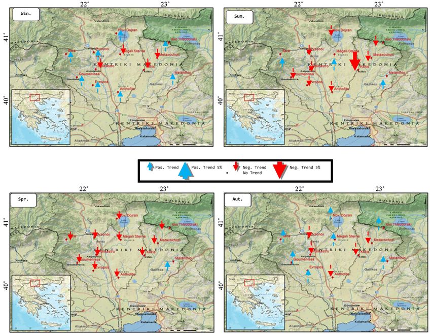
In four seasons analysis, as it can be seen from Figure 6, in the winter season
mainly upward trends where observed while in spring downward ones in most
stations. The summer showed only three upward trends while a statistically sig-
nificant downward trend at 5% significance level is identified only in the Kilkis
DOI: 10.4236/cweee.2021.102004 58 Computational Water, Energy, and Environmental EngineeringA. K. Margaritidis
Figure 4. Sen’s estimator of slope at Kilkis station (annual scale).
Figure 5. Trend results with non-parametric test Mann-Kendall at 12 stations in the
study area during the irrigation period.
Figure 6. Seasonal trend results with non-parametric test Mann-Kendall at 12 stations in the study area.
DOI: 10.4236/cweee.2021.102004 59 Computational Water, Energy, and Environmental EngineeringA. K. Margaritidis
station (Figure 6). In autumn, both downward and upward not statistically sig-
nificant trends occurred (Table 6).
Concerning the trend slopes of precipitation in seasonal period analysis, the
statistically significant downward trend slope of Kilkis station was estimated as
equal to 2.1 mm/season at a significance level of 5% as shown in Figure 7 and
Table 7.
Table 6. Seasonal trend results of precipitation with Mann-Kendall, Spearman and Sen’s-T tests in the study area.
Mann-Kendall/Spearman/Sen-T
(**) 1 2 3 4
Total Precip. Μ-Κ Spearman Μ-Κ Spearman Μ-Κ Spearman Μ-Κ Spearman
Sen-Τ Sen-Τ Sen-Τ Sen-Τ
(1973-2008) Test Z p value Test Z p value Test Z p value Test Z p value
Winter 1.10 0.243 1.178 0.10 0.865 0.184 −1.05 0.253 −1.154 −1.13 0.269 −1.116
Spring −0.42 0.569 −0.579 −1.51 0.117 −1.575 −0.68 0.494 −0.694 −1.40 0.135 −1.500
Summer −0.15 0.962 −0.049 −0.10 0.889 −0.143 −1.19 0.262 −1.133 −2.15* 0.037* −2.067*
Autumn 0.40 0.547 0.611 1.09 0.385 0.880 −0.25 0.906 −0.120 −1.05 0.350 −0.946
(**) 5 6 7 8
Winter 0.59 0.376 0.895 0.53 0.535 0.629 −0.31 0.969 0.040 1.62 0.074 1.783
Spring 0.90 0.278 1.095 −1.01 0.295 −1.059 −0.68 0.455 −0.758 −1.31 0.198 −1.297
Summer 1.62 0.128 1.529 −1.32 0.155 −1.430 0.19 0.974 0.033 −0.19 0.895 −0.135
Autumn 1.44 0.151 1.443 −0.59 0.556 −0.599 0.72 0.502 0.681 −0.10 0.851 −0.192
(**) 9 10 11 12
Winter −0.37 0.693 −0.402 0.16 0.589 0.549 0.42 0.548 0.609 0.91 0.329 0.987
Spring −0.56 0.575 −0.570 −0.89 0.330 −0.987 −1.40 0.216 −1.249 −0.84 0.399 −0.855
Summer −0.56 0.477 −0.722 −1.55 0.127 −1.531 −0.53 0.534 −0.632 0.18 0.758 0.313
Autumn −0.86 0.302 −1.043 0.16 0.738 0.340 0.42 0.707 0.382 0.01 0.931 0.088
* Statistically significant at the 5% level of significance. ** 1. Nov. Dojran. 2. Ano Theodoraki. 3. Metaxochori. 4. Kilkis. 5. Melanthio. 6. Anthofito. 7. Μegali
Sterna. 8. Εvzonoi. 9. Polikastro. 10. Evropos. 11. Goumenissa. 12. Skra.
Table 7. Seasonal trend results of the slope of the precipitation trend in the study area.
Sen’s Estimate Slope (mm/period)
(
** )
1. 2. 3. 4. 5. 6. 7. 8. 9. 10. 11. 12.
Precipitation Μ-Κ Μ-Κ Μ-Κ Μ-Κ Μ-Κ Μ-Κ Μ-Κ Μ-Κ Μ-Κ Μ-Κ Μ-Κ Μ-Κ
(1973-2008) Test Q Test Q Test Q Test Q Test Q Test Q Test Q Test Q Test Q Test Q Test Q Test Q
Winter 1.166 0.134 −1.051 −0.738 0.802 0.601 −0.209 2.538 −0.460 0.220 0.761 1.771
Spring −0.461 −1.130 −0.546 −1.124 0.844 −0.752 −0.605 −1.300 −0.371 −0.816 −1.906 −1.118
Summer −0.153 −0.101 −1.457 −2.09* 2.102 −1.241 0.288 −0.224 −0.438 −1.892 −0.689 0.089
Autumn 0.666 0.897 −0.345 −0.897 1.795 −0.978 0.535 −0.186 −1.191 0.322 1.066 0.092
* Statistically significant at the 5% level of significance. ** 1. Nov. Dojran. 2. Ano Theodoraki. 3. Metaxochori. 4. Kilkis. 5. Melanthio. 6. Anthofito. 7. Megali
Sterna. 8. Evzonoi. 9. Polikastro. 10. Evropos. 11. Goumenissa. 12. Skra.
DOI: 10.4236/cweee.2021.102004 60 Computational Water, Energy, and Environmental EngineeringA. K. Margaritidis
Figure 7. Sen’s estimator of slope at Kilkis station (summer period).
On a monthly basis, the trend in the examined stations has appeared in several
time series statistically significant at 5% significance level. In Table 8 the trend
sign results of the non-parametric Mann-Kendall, Sen-T και Spearman Rho tests
are presented. October showed an equal number of negative and positive trends.
November was identified as a month with a negative trend of precipitation in all
stations except Melanthio and Skra station which showed upward trends. The
Anthofito station showed a statistically significant positive slope trend at a 5%
level of significance. The month of December is characterized as a month of pos-
itive trend precipitation but only Skra station was identified statistically signifi-
cant at a significance level of 5%. January showed both positive and negative
trends. February showed mostly downward trends while not statistically signifi-
cant. Negative and not statistically significant were the trends in all stations in
March as well. In April, both negative and positive trends which were also not
statistically significant were calculated.
In May, only two stations presented upward trend but non-statistically signif-
icant while the remaining stations showed downward trend with only the Ano
Theodoraki station identified as statistically significant at 5% level of signific-
ance. No prevailing trend direction could characterize the months of June and
July. In August, two statistically significant trends were identified in stations
Evropos and Kilkis at significance level of 5%. Finally, during the last month of
hydrological year (September) Megali Sterna, Melanthio and Evzonoi revealed
statistically significant downward trends. Comparing the results of the three
trend tests (Table 8), it can be noted that the all stations for all time periods of
study, the trends show the same sign behavior with a few exceptions. The trend
slope of time series that were found statistically significant trends is presented in
Figure 8. As it can be observed the maximum positive slope value is 1.99
mm/month at Skra station in December while the maximum negative slope val-
ue is 1.00 mm/month at Ano Theodoraki station in May which is a crucial
month for irrigation purposes.
Table 8. Total results of the sign of precipitation trend in the study area.
Mann-Kendall-Sen’s T-Spearman (5% S. L)
Nov. Dojran Ano Theodoraki Metaxochori Kilkis
Total M-K Sen’s Spearman M-K Sen’s Spearman M-K Sen’s Spearman M-K Sen’s Spearman
Precipitation Ζ T ρ Ζ T ρ Ζ T ρ Ζ T ρ
Annual + + + - - - - - - -* -* -*
DOI: 10.4236/cweee.2021.102004 61 Computational Water, Energy, and Environmental EngineeringA. K. Margaritidis
Continued
Winter + + + + + + - - - - - -
Spring - - - - - - - - - - - -
Summer - - - - - - - - - -* -* -*
Autumn + + + + + + - - - - - -
Irrig. Period + + + - - - - - - - - -
October + + + + + + + - - - - -
November - - - - - - - - - - - -
December + + + + + + + + + + + +
January + + + + + + - - - - - -
February - - - - - - - - - - - -
March - - - - - - - - - - - -
April + + + - - - + + + - - -
May - - - -* -* -* - - - - - -
June + + + + + + - - - - - -
July - - - - + + - - - - - -
August - - - - - - - - - -* -* -*
September + + + + + + + + + + + +
Melanthio Anthofito Megali Sterna Evzonoi
Total Sen’s Spearman Sen’s Spearman Sen’s Spearman Sen’s Spearman
M-K Ζ M-K Ζ M-K Ζ M-K Ζ
Precipitation T ρ T ρ T ρ T ρ
Annual + + + - - - - - - - + +
Winter + + + + + + - + + + + +
Spring + + + - - - - - - - - -
Summer + + + - - - + + + - - -
Autumn + + + - - - + + + - - -
Irrig. Period + + + - - - + + + + + +
October + + + 0 - - - - - + + +
November + + + -* -* -* - - - - - -
December + + + + - - + + + + + +
January + + + + + + + + + + + +
February - - - - - - - - - - - -
March - - - - - - - - - - - -
April + + + + + + + + + - - -
May + + + - - - - - - - - -
June + + + - - - 0 + + 0 - -
July + + + - - - + + + - - -
August + + + - - - + + + - - -
September +* +* +* + + + +* +* +* +* +* +*
Polikastro Evropos Goumenissa Skra
Total Sen’s Spearman Sen’s Spearman Sen’s Spearman Sen’s Spearman
M-K Ζ M-K Ζ M-K Ζ M-K Ζ
Precipitation T ρ T ρ T ρ T ρ
Annual - - - - - - + + + + + +
Winter - - - + + + + + + + + +
DOI: 10.4236/cweee.2021.102004 62 Computational Water, Energy, and Environmental EngineeringA. K. Margaritidis
Continued
Spring - - - - - - - - - - - -
Summer - - - - - - - - - + + +
Autumn - - - + + + + + + + + +
Irrig. Period - - - - - - - - - + + +
October - - - + + + - - - - - -
November - - - - - - - - - + + +
December + + + + + + + + + +* +* +*
January - - - + + + 0 + + + + +
February - - - + + + - - - - - -
March - - - - - - - - - - - -
April 0 + 0 - - - + + + + + +
May + + + - - - - - - - - -
June - - - - - - - - - + + +
July - - - - - - + + + + + +
August - - - -* -* -* - - - - - -
September - - - + + + + + + - - -
*Statistically significance at the 5% level of significance.
Figure 8. Monthly statistically significant trends at station level in the study area (5% lev-
el of significance).
DOI: 10.4236/cweee.2021.102004 63 Computational Water, Energy, and Environmental EngineeringA. K. Margaritidis
3.2. Regional Trend Analysis
The investigation of precipitation trends in the area was performed by the Re-
gional Average Mann-Kendall (RAMK) test. Furthermore, in order to assess the
field significance, the spatial RAMK trend test was evaluated with the Bootstrap
Empirical Cumulative Distribution (BECD). The bootstrap RAMK test was ela-
borated in two versions: with and without preserving cross-correlation.
As it concerns the RAMK test, the region showed a downward trend of preci-
pitation during the annual period which was not found to be statistically signifi-
cant. Same trend sign, but weaker has appeared during the irrigation period. Sta-
tistically significant at 5% and 10% significance level were estimated the trends
at regional level in the seasons of spring and summer respectively (Table 9). The
winter and autumn seasons were characterized as seasons with upward trend,
not statistically significant according to the results of Table 9.
In the monthly observations, the spatial trends showed a larger statistical in-
terest, as the 58.3% of them was determined to be statistically significant at a sig-
nificance level of 5% (Table 9). In detail, the months of November, February,
March, May and August have downward trends at 5% significance level. Con-
trary, the months September and December showed significant upward trends
and slopes at a significance level of 5%.
The analysis of trends in the region, in order to assess the field significance, is
investigated using RAMK Bootstrap test without (RAMK-B1) and with (RAMK-B2)
preserving the cross correlation. For each time period of observation, 4.000 ran-
dom repetitions were conducted and 4.000 values of S statistic were calculated.
In Table 9, the results of the two bootstrap RAMK tests are presented. The effect
of spatial correlation at the level of significance of 5% can be clearly seen by
comparing the results of the trend of the two tests (Figure 9), while the BECD’s
without and with cross correlation is shown in Figure 10.
Table 9. RAMK test results and RAMK-B (1, 2) at 5% (bold) and 10% (italics) level of significance respectively.
RAMK-B1 test RAMK-B2 test
RAMK test
Field Significance (without cross correlation) (with cross correlation)
S av. Pobs Pf Z Pobs Pf Pobs Pf
Annual −33.6 0.113 0.113 −1.59 0.058 0.058 0.181 0.181
Irrig. −20.4 0.337 0.337 −0.96 0.177 0.177 0.327 0.327
Winter 26.4 0.214 0.214 1.24 0.898 0.102 0.689 0.311
Spring −60.8 0.004 0.004 −2.87 0.002 0.002 0.083 0.083
Summer −35.6 0.094 0.094 −1.68 0.048 0.048 0.260 0.260
Autumn 8.83 0.680 0.320 0.41 0.676 0.324 0.586 0.414
Oct. 4.66 0.829 0.171 0.22 0.570 0.430 0.534 0.466
Nov. −73.1 0.001 0.001 −3.45 0.001 0.001 0.096 0.096
Dec. 64.5 0.002 0.002 3.04 1.000 0.000 0.891 0.109
Jan. 17.3 0.414 0.414 0.82 0.790 0.210 0.677 0.323
DOI: 10.4236/cweee.2021.102004 64 Computational Water, Energy, and Environmental EngineeringA. K. Margaritidis
Continued
Feb. −64.6 0.002 0.002 −3.05 0.002 0.002 0.109 0.109
March −76.9 0.000 0.000 −3.63 0.000 0.000 0.060 0.060
Apr. 5.7 0.792 0.208 0.26 0.624 0.376 0.529 0.471
May −57.7 0.005 0.005 −2.79 0.004 0.004 0.112 0.112
June −2.9 0.894 0.106 −0.13 0.446 0.446 0.466 0.466
July −22 0.300 0.300 −1.04 0.153 0.153 0.338 0.338
Aug. −60.1 0.005 0.005 −2.84 0.001 0.001 0.091 0.091
Sept. 87.2 0.000 0.000 4.11 1.000 0.000 0.963 0.037
Figure 9. Charts comparing RAMK test and RAMK-Β (1, 2) tests at regional level for
time study periods.
Figure 10. The annual bootstrap empirical cdf curve for the region with the effect of cross
correlation (S’) and without (S).
In the monthly observations, the spatial trends showed a larger statistical in-
terest, as the 58.3% of them was determined to be statistically significant at a sig-
nificance level of 5% (Table 9). In detail, the months of November, February,
DOI: 10.4236/cweee.2021.102004 65 Computational Water, Energy, and Environmental EngineeringA. K. Margaritidis
March, May and August have downward trends at 5% significance level. Con-
trary, the months September and December showed significant upward trends
and slopes at a significance level of 5%.
The analysis of trends in the region, in order to assess the field significance, is in-
vestigated using RAMK Bootstrap test without (RAMK-B1) and with (RAMK-B2)
preserving the cross correlation. For each time period of observation, 4.000 ran-
dom repetitions were conducted and 4.000 values of S statistic were calculated.
In Table 9, the results of the two bootstrap RAMK tests are presented. The effect
of spatial correlation at the level of significance of 5% can be clearly seen by
comparing the results of the trend of the two tests (Figure 9), while the BECD’s
without and with cross correlation is shown in Figure 10.
As illustrated in Figure 9, the negative trend in the region during the annual
period appears statistically significant at the level of significance of 10% (Table
9) only with RAMK-B1 test, fact which was not verified with the corresponding
tests RAMK and RAMK-B2 respectively. This reinforces the hypothesis of cross
correlation existence in the historical time series whose results converge with
those of test RAMK-B2. The annual bootstrap empirical cdf curves with and
without cross correlation show the effect of cross correlation in the identification
of field significance (Figure 10).
The results of spatial trends in precipitation during the periods of winter, au-
tumn and irrigation showed no statistically significant trend for all tests. How-
ever, the season of spring was characterized by statistically significant downward
trend (Table 9 and Figure 9) at significance level of 5% with the tests RAMK
and RAMK-B1, which was verified by RAMK-B2 but at 10% significance level.
Finally, during the season of summer the spatial test RAMK-B1 detected trends
at significance level of 5% while test RAMK at a significance level of 10%.
In monthly observations, the RAMK-B2 has also identified fewer trends com-
pared to RAMK-B1 (Figure 9). Similar, regarding the effect of the cross correla-
tion with bootstrap tests, were the results [32] in the analysis of the minimum
annual, mean annual and maximum annual daily flow in Canada.
In this study, both RAMK-B tests estimated negative precipitation trends in
the months November, August and March which were statistically significant at
a significance level of 5% and 10% for RAMK-B1 and RAMK-B2 tests respec-
tively. The most important upward trend in the region was identified by both
tests in September at significance level 5%. Also, an upward trend is detected in
December with RAMK-B1 test while it was not verified with RAMK-B2 test. It is
noted that for both negative and positive spatial trends identified by RAMK-B1
test were also found by the RAMK test of the historical time series. In most cases
the RAMK-B2 test identified fewer field significances of trend than the corres-
ponding RAMK-B1, with the exception of month January and the irrigation pe-
riod.
4. Conclusions
At station level, the results produced by Mann-Kendall test, Sen’s T test, Sen’s
DOI: 10.4236/cweee.2021.102004 66 Computational Water, Energy, and Environmental EngineeringA. K. Margaritidis
estimate of slope test and Spearman test were highly consistent for all time
scales. The precipitation trend according to the tests mentioned above appeared
in most cases downward during the annual analysis and statistically significant
at 5% level of significance only in one station. In seasonal analysis, statistically
significant (5% s.l.) was detected also only at one station with a downward pre-
cipitation trend during the summer period. Comparing the results at a monthly
scale in all stations, several statistically significant trends were found at a few
numbers of stations. The station Nov. Doiran on the part of F.Y.R.O.M. did not
show at station level a statistically significant negative or positive precipitation
trend at any of the recording time periods, except for mild negative and positive
trends and inclinations respectively. Greater mild negative non-statistically sig-
nificant trend occurred during spring. This may signal the fact that there have
not been long periods of minimum water availability in Lake Doirani’s basin
through precipitation. Thus, variables such as wind temperature and velocity
may have contributed to increased evaporation and reduced soil moisture. As a
result, significant droughts occur in the lake, especially from 1973 to 2002 [34].
At a regional level, RAMK-B2 test revealed statistically significant positive
trends in precipitation at 5% significance level only during September. In addi-
tion, statistically significant negative spatial trends were observed in the season
of spring and at 10% significance level for the months November, March and
August. Instead, the RAMK-B1 test estimated negative spatial trends statistically
significant at a significance level of 5% for the seasons of spring and summer as
well as for the months of November, February, March, May and August. Also, a
negative trend was identified for the annual period at significance level of 10%.
Positive spatial trends at 5% significance level were observed during December
(RAMK, RAMK-B1) and September with all spatial tests, respectively. Overall,
the trend of precipitation was statistically significant at a level of 10% only with
RAMK-1 control during the annual period while 5% in spring [35] and summer
[34] in RAMK and RAMK-1 control respectively. For all examined time periods,
the RAMK test showed statistically significant spatial trends at significance level
of 5% at a rate of 44.4% (8/18), the RAMK-B1 test at a rate of 50% (9/18), while
the RAMK-B2 test at a rate of 5.5% (1/18). Extending the significance level to
10%, the RAMK test showed statistically significant spatial trends at a rate of
50% (9/18), the RAMK-B1 test at a rate of 55.5% (10/18), while the RAMK-B2
test at a rate of % 27.7 (5/18). Comparing the results of the two bootstrap tests, it
is highlighted that field significance of trends in the study area is influenced by
the effect of cross-correlation between the stations.
Closing, the spatial inspections, with the exception of the RAMK-2 test,
showed a wealth of statistically significant and less statistically significant trends,
which is confirmed by other researchers too on precipitation trends in the sur-
rounding area and in Greece in general [36] [37].
Acknowledgements
I would like to thank the local Department of Land Reclamation of Kilkis (Minis-
DOI: 10.4236/cweee.2021.102004 67 Computational Water, Energy, and Environmental EngineeringA. K. Margaritidis
try of Environment, Energy and Climate Change) and the Greek Biotope/Wetland
Centre for the provision of precipitation data. In conclusion, i would like to
thank my mother Margaritidou Anastasia for her help both in the collection of
data and in the recording, as well as in the psychological support during the
whole process of this research.
Conflicts of Interest
The author declares no conflicts of interest regarding the publication of this pa-
per.
References
[1] Gemmer, M., Becker, S. and Jiang, T. (2004) Observed Monthly Precipitation
Trends in China 1951-2002. Theoretical and Applied Climatology, 77, 39-45.
https://doi.org/10.1007/s00704-003-0018-3
[2] Parry, M.L., Canziani, O., Palutikof, J., Van Der Linden, P. and Hanson, C. (2007)
IPCC Climate Change 2007: Impacts, Adaptation and Vulnerability. Contribution
of Working Group II to the Fourth Assessment Report of the Intergovernmental
Panel on Climate Change. Cambridge University Press, Cambridge, UK, 976.
[3] Xu, L., Zhou, H., Du, L., Yao, H. and Wang, H. (2015) Precipitation Trends and Va-
riability from 1950 to 2000 in Arid Lands of Central Asia. Journal of Arid Land, 7,
514-526. https://doi.org/10.1007/s40333-015-0045-9
[4] Hu, Y., Wang, S., Song, X. and Wang, J. (2017) Precipitation Changes in the
Mid-Latitudes of the Chinese Mainland during 1960-2014. Journal of Arid Land, 9,
924-937. https://doi.org/10.1007/s40333-017-0105-4
[5] Wu, Y., Bake, B., Zhang, J. and Rasulov, H. (2015) Spatio-Temporal Patterns of
Drought in North Xinjiang, China, 1961-2012 Based on Meteorological Drought
Index. Journal of Arid Land, 7, 527-543. https://doi.org/10.1007/s40333-015-0125-x
[6] Yue, S. and Wang, C.Y. (2002) Regional Streamflow Trend Detection with Consid-
eration of Both Temporal and Spatial Correlation. International Journal of Clima-
tology, 22, 933-946. https://doi.org/10.1002/joc.781
[7] Buffoni, L., Maugeri, M. and Nanni, T. (1999) Precipitation in Italy from 1833 to
1996. Theoretical and Applied Climatology, 63, 33-40.
https://doi.org/10.1007/s007040050089
[8] Piccarreta, M., Capolongo, D. and Boenzi, F. (2004) Trend Analysis of Precipitation
and Drought in Basilicata from 1923 to 2000 within a Southern Italy Context. In-
ternational Journal of Climatology, 24, 907-922. https://doi.org/10.1002/joc.1038
[9] Partal, T. and Kahya, E. (2006) Trend Analysis in Turkish Precipitation Data. Hy-
drological Processes, 20, 2011-2026. https://doi.org/10.1002/hyp.5993
[10] Cannarozzo, M., Noto, L.V. and Viola, F. (2006) Spatial Distribution of Rainfall
Trends in Sicily (1921-2000). Physics and Chemistry of the Earth, Parts A/B/C, 31,
1201-1211. https://doi.org/10.1016/j.pce.2006.03.022
[11] Smadi, M.M. and Zghoul, A. (2006) A Sudden Change in Rainfall Characteristics in
Amman, Jordan during the Mid1950s. American Journal of Environmental Sciences,
2, 84-91.
[12] De Lima, M.I.P., Marques, A.C., De Lima, J.L.M.P. and Coelho, M.F.E.S. (2007)
Precipitation Trends in Mainland Portugal in the Period 1941-2000. In: Lobo Fer-
reira, J.P. and Viera, J.M.P., Eds., Water in Celtic Countries: Quantity, Quality and
DOI: 10.4236/cweee.2021.102004 68 Computational Water, Energy, and Environmental EngineeringA. K. Margaritidis
Climate Variability, International Association of Hydrological Sciences, Walling-
ford, 94-102.
[13] Chaouche, K., Neppel, L., Dieulin, C., Pujol, N., Ladouche, B., Martin, E. and Ca-
ballero, Y. (2010) Analyses of Precipitation, Temperature and Evapotranspiration in
a French Mediterranean Region in the Context of Climate Change. Comptes Ren-
dus Geoscience, 342, 234-243. https://doi.org/10.1016/j.crte.2010.02.001
[14] Luna, M.Y., Guijarro, J.A. and López, J.A. (2012) A Monthly Precipitation Database
for Spain (1851-2008): Reconstruction, Homogeneity and Trends. Advances in
Science and Research, 8, 1-4. https://doi.org/10.5194/asr-8-1-2012
[15] Dalezios, N.R. and Bartzokas, A. (1995) Daily Precipitation Variability in Semiarid
Agricultural Regions in Macedonia, Greece. Hydrological Sciences Journal, 40, 569-585.
https://doi.org/10.1080/02626669509491445
[16] Kambezidis, H.D., Larissi, I.K., Nastos, P.T. and Paliatsos, A.G. (2010) Spatial Va-
riability and Trends of the Rain Intensity over Greece. Advances in Geosciences, 26,
65-69. https://doi.org/10.5194/adgeo-26-65-2010
[17] Karpouzos, D.K., Kavalieratou, S. and Babajimopoulos, C. (2010) Trend Analysis of
Precipitation Data in Pieria Region (Greece). European Water, 30, 31-40.
[18] Nastos, P.T. and Zerefos, C.S. (2010) Climate Change and Precipitation in Greece.
Hellenic Journal of Geosciences, 45, 185-192.
[19] Myronidis, D., Stathis, D., Ioannou, K. and Fotakis, D. (2012) An Integration of Sta-
tistics Temporal Methods to Track the Effect of Drought in a Shallow Mediterra-
nean Lake. Water Resources Management, 26, 4587-4605.
https://doi.org/10.1007/s11269-012-0169-z
[20] Matalas, N.C. and Jacobs, B. (1964) A Correlation Procedure for Augmenting Hy-
drologic Data. US Government Printing Office, 434, 1-13.
https://doi.org/10.3133/pp434E
[21] Margaritidis, K.A and Karpouzos, K.D. (2015) Homogeneity of Rainfall Time Series
Analysis in the Wider Area of Doiran. Proceedings of the 9th Panhellenic Confe-
rence of Agricultural Engineering, Thessaloniki, 8-9 October 2015, 123-132.
[22] Rai, R.K., Upadhyay, A. and Ojha, C.S.P. (2010) Temporal Variability of Climatic
Parameters of Yamuna River Basin: Spatial Analysis of Persistence, Trend and Pe-
riodicity. The Open Hydrology Journal, 4, 184-210.
https://doi.org/10.2174/1874378101004010184
[23] Yue, S., Pilon, P. and Cavadias, G. (2002) Power of the Mann-Kendall and Spear-
man’s Rho Tests for Detecting Monotonic Trends in Hydrological Series. Journal of
Hydrology, 259, 254-271. https://doi.org/10.1016/S0022-1694(01)00594-7
[24] Eymen, A. and Köylü, Ü. (2018) Seasonal Trend Analysis and ARIMA Modeling of
Relative Humidity and Wind Speed Time Series around Yamula Dam. Meteorology
and Atmospheric Physics, 131, 601-612. https://doi.org/10.1007/s00703-018-0591-8
[25] Sen, P.K. (1968) On a Class of Aligned Rank Order Tests in Two-Way Layouts. The
Annals of Mathematical Statistics, 39, 1115-1124.
https://doi.org/10.1214/aoms/1177698236
[26] Sen, P.K. (1968) Estimates of the Regression Coefficient Based on Kendall’s Tau.
Journal of the American Statistical Association, 63, 1379-1389.
https://doi.org/10.1080/01621459.1968.10480934
[27] Van Belle, G. and Hughes, J.P. (1984) Nonparametric Tests for Trend in Water
Quality. Water Resources Research, 20, 127-136.
https://doi.org/10.1029/WR020i001p00127
DOI: 10.4236/cweee.2021.102004 69 Computational Water, Energy, and Environmental EngineeringA. K. Margaritidis
[28] Douglas, E.M., Vogel, R.M. and Kroll, C.N. (2000) Trends in Floods and Low Flows
in the United States: Impact of Spatial Correlation. Journal of Hydrology, 240,
90-105. https://doi.org/10.1016/S0022-1694(00)00336-X
[29] Helsel, D.R. and Frans, L.M. (2006) Regional Kendall Test for Trend. Environmen-
tal Science and Technology, 40, 4066-4073. https://doi.org/10.1021/es051650b
[30] Palizdan, N., Falamarzi, Y., Huang, Y.F., Lee, T.S. and Ghazali, A.H. (2014) Region-
al Precipitation Trend Analysis at the Langat River Basin, Selangor, Malaysia.
Theoretical and Applied Climatology, 117, 589-606.
https://doi.org/10.1007/s00704-013-1026-6
[31] Yue, S. and Hashino, M. (2003) Long Term Trends of Annual and Monthly Precipi-
tation in Japan. JAWRA Journal of the American Water Resources Association, 39,
587-596. https://doi.org/10.1111/j.1752-1688.2003.tb03677.x
[32] Yue, S., Pilon, P. and Phinney, B.O.B. (2003) Canadian Streamflow Trend Detec-
tion: Impacts of Serial and Cross-Correlation. Hydrological Sciences Journal, 48,
51-63. https://doi.org/10.1623/hysj.48.1.51.43478
[33] Mann, H.B. (1945) Nonparametric Tests against Trend. Econometrica, 13, 245-259.
https://doi.org/10.2307/1907187
[34] Myronidis, D. (2010) Research of the Causes in the Drop of Lake Doirani’s Water
Level (Greece) and Elaboration of a Pilot Action Plan for Its Restoration, Final Re-
port. State Scholarship Foundation, Greece, 79.
[35] Ruixia, G., Clara, D., Laurent, T. and Flavio, L. (2019) Human Influence on Winter
Precipitation Trends (1921-2015) over North America and Eurasia. Revealed by
Dynamical Adjustment. Geophysical Research Letters, 46, 3426-3434.
https://doi.org/10.1029/2018GL081316
[36] Mavromatis, T. and Stathis D. (2011) Response of the Water Balance in Greece to
Temperature and Precipitation Trends. Theoretical and Applied Climatology, 104,
13-24. https://doi.org/10.1007/s00704-010-0320-9
[37] Feidas, X., Noulopoulou, C., Makrogiannis, T. and Bora-Senta, E. (2007) Trend
Analysis of Precipitation Time Series in Greece and Their Relationship with Circu-
lation Using Surface and Satellite Data: 1955-2001. Theoretical and Applied Clima-
tology, 87, 155-177. https://doi.org/10.1007/s00704-006-0200-5
DOI: 10.4236/cweee.2021.102004 70 Computational Water, Energy, and Environmental EngineeringYou can also read