Non-Stationary Flood Frequency Analysis Using Cubic B-Spline-Based GAMLSS Model - MDPI
←
→
Page content transcription
If your browser does not render page correctly, please read the page content below
water
Article
Non-Stationary Flood Frequency Analysis Using
Cubic B-Spline-Based GAMLSS Model
Chunlai Qu 1 , Jing Li 1 , Lei Yan 1,2, *, Pengtao Yan 3 , Fang Cheng 1 and Dongyang Lu 1
 1   College of Water Conservancy and Hydropower, Hebei University of Engineering, Handan 056021, China;
     quchunlai@hebeu.edu.cn (C.Q.); lijing1996xt@163.com (J.L.); chengfang12386@163.com (F.C.);
     ludongyang1996@163.com (D.L.)
 2   State Key Laboratory of Water Resources and Hydropower Engineering Science, Wuhan University,
     Wuhan 430072, China
 3   School of Physics and Electronic Engineering, Xingtai University, Xingtai 054001, China; mryanpt@163.com
 *   Correspondence: yanl@whu.edu.cn; Tel.: +86-178-3100-3218

 Received: 12 May 2020; Accepted: 22 June 2020; Published: 29 June 2020

 Abstract: Under changing environments, the most widely used non-stationary flood frequency
 analysis (NFFA) method is the generalized additive models for location, scale and shape (GAMLSS)
 model. However, the model structure of the GAMLSS model is relatively complex due to the large
 number of statistical parameters, and the relationship between statistical parameters and covariates is
 assumed to be unchanged in future, which may be unreasonable. In recent years, nonparametric
 methods have received increasing attention in the field of NFFA. Among them, the linear quantile
 regression (QR-L) model and the non-linear quantile regression model of cubic B-spline (QR-CB)
 have been introduced into NFFA studies because they do not need to determine statistical parameters
 and consider the relationship between statistical parameters and covariates. However, these two
 quantile regression models have difficulties in estimating non-stationary design flood, since the trend
 of the established model must be extrapolated infinitely to estimate design flood. Besides, the number
 of available observations becomes scarcer when estimating design values corresponding to higher
 return periods, leading to unreasonable and inaccurate design values. In this study, we attempt to
 propose a cubic B-spline-based GAMLSS model (GAMLSS-CB) for NFFA. In the GAMLSS-CB model,
 the relationship between statistical parameters and covariates is fitted by the cubic B-spline under the
 GAMLSS model framework. We also compare the performance of different non-stationary models,
 namely the QR-L, QR-CB, and GAMLSS-CB models. Finally, based on the optimal non-stationary
 model, the non-stationary design flood values are estimated using the average design life level
 method (ADLL). The annual maximum flood series of four stations in the Weihe River basin and
 the Pearl River basin are taken as examples. The results show that the GAMLSS-CB model displays
 the best model performance compared with the QR-L and QR-CB models. Moreover, it is feasible to
 estimate design flood values based on the GAMLSS-CB model using the ADLL method, while the
 estimation of design flood based on the quantile regression model requires further studies.

 Keywords: non-stationarity; B-spline; GAMLSS-CB; quantile regression; flood frequency analysis;
 design flood

1. Introduction
     Flood frequency analysis is very important for the construction of hydrological projects.
The stationary assumption has served as the basic assumption in flood frequency analysis for decades.
However, due to climate change and human activities, the spatial and temporal distribution of rainfall
and the catchment conditions have been changed. The stationary assumption has been challenged by

Water 2020, 12, 1867; doi:10.3390/w12071867                                       www.mdpi.com/journal/water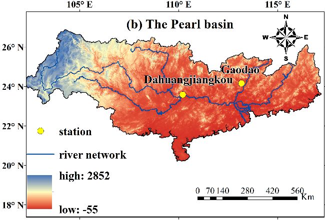
Water 2020, 12, 1867                                                                                 2 of 17

many researchers [1–13] and the rationality of the design results obtained by traditional stationary
flood frequency analysis has been questioned [6,14]. Therefore, the non-stationary frequency analysis
of flood series under changing environments is of great significance to ensure the rationality of flood
design results [1,11–15]. There are several well-written articles summarizing the existing methods
for non-stationary flood frequency analysis (NFFA) [8,16–19]. NFFA has become one of the research
hotspots in the field of flood frequency analysis under changing environments.
      The generalized additive models for location, scale and shape (GAMLSS) model is currently the
most commonly used method in NFFA [5,6,20–25]. However, due to the large number of statistical
parameters and the complexity of the relationship between statistical parameters and covariates,
the model structure of GAMLSS is relatively complex. At the same time, the GAMLSS model assumes
that the relationship between statistical parameters and covariates will remain unchanged in future,
which may be unreasonable. In recent years, nonparametric methods have received more and more
attention in the field of hydrological analysis and calculation. The simple linear quantile regression
(QR-L) model in particular has been employed in NFFA. This is mainly because the QR-L model
does not need to determine statistical parameters and consider the relationship between statistical
parameters and covariates, which can definitely simplify the process of model construction. Koenker
and Basset [26] first proposed the quantile regression method, and then it was introduced into the field
of hydrological frequency analysis. Barbosa [27] used quantile regression to analyze Baltic Sea level
change and found that the slope at the maximum value was more significant. Mazvimavi [28] used the
quantile regression method to analyze changes in the rainfall series in Zimbabwe, and then found that
climate change effects were not yet statistically significant within the time series of total seasonal and
annual rainfall in Zimbabwe. Wang et al. [29] analyzed the possible changes in monthly precipitation
in the southern United States using quantile regression. Feng et al. [30] used the quantile regression
method to analyze the variation characteristics of the annual precipitation and runoff series in the
Luanhe River Basin, and found that the annual runoff series in the sub-basin was no longer stationary.
      However, in the field of hydrological frequency analysis, the dependence between the covariate
and the independent variable is complex so it is unreasonable to simply use linearity, and more
complex statistical relations between covariates and independent variables need to be considered [31].
The non-linear quantile regression model of cubic B-spline (QR-CB) was recommended in NFFA by
Nasri et al. [31]. Compared with the QR-L model, the QR-CB model is more reasonable. The construction
of the cubic B-spline function is only related to the number and position of the nodes and the degree of
freedom of the function, and is not affected by the variables, so the model is more robust. Hendricks
and Koenker [32] proposed spline parameterization using conditional quantile functions to estimate
household electricity demand in metropolitan areas of Chicago. Nasri et al. [33] established a Generalized
Extreme Value (GEV) model with a cubic B-spline curve under the Bayesian framework, and suggested
that in future we can focus on the comparison of the extreme value model with the regression quantiles
in order to use different covariates in quantile estimation. Nasri et al. [31] used cubic B-spline quantile
regression to perform a non-stationary hydrological frequency analysis of the annual maximum and
minimum flow records for Ontario, Canada.
      However, it is difficult to estimate flood design values based on either the QR-L or QR-CB models.
Currently, there is no accurate method for estimating the design flood values based on the quantile
regression model. On the contrary, researchers have developed several non-stationary design methods
when using the GAMLSS model [34–39]. Yan et al. [38] compared different design methods and
recommended both equivalent reliability (ER) and average design life level (ADLL) for practical use
because the design floods estimated by these two methods are linked with the design life of projects
and possess reasonable confidence intervals.
      Some researchers have tried to build a non-linear GAMLSS model for NFFA, and the results have
shown that compared with the stationary model, variation types such as cubic spline function and
parabolic function possess a better performance [22,40,41]. In this study, we attempted to develop a
cubic B-spline-based GAMLSS model (GAMLSS-CB) by combining the GAMLSS model with the cubic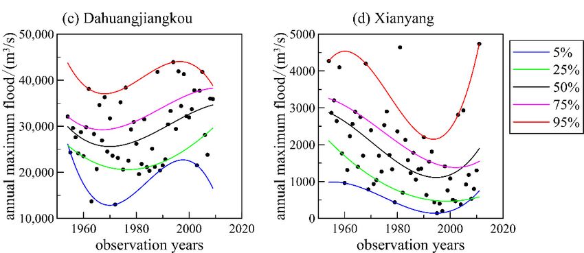
Water 2020, 12, 1867                                                                                           3 of 17

B-spline. In the GAMLSS-CB model, the relationship between statistical parameters and covariates was
fitted by the cubic B-spline under the GAMLSS model framework. We then compared its difference from
the QR-L and QR-CB models. In this paper, the annual maximum flood series of four representative
stations in the Weihe River Basin and the Pearl River Basin were selected as the research objects.
The flood series of these stations are representative because they are located in different climate
regions of China and exhibited either increasing or decreasing trends. Finally, based on the optimal
non-stationary model, we also estimated the non-stationary design flood values using the ADLL
method proposed by Yan et al. [25,38].
      The paper is organized as follows: the second section introduces the methodologies, the third
section gives the study areas and data, the fourth section gives the results, the fifth section is the
discussion, and the sixth section is the conclusions.

2. Methodologies

2.1. Mann–Kendall Trend Test Method
     The Mann–Kendall nonparametric trend test method was used to detect the long-term change
trend of the precipitation and runoff series. This method has no need for the sample series to obey
a specific distribution, and is not disturbed by a few outliers. It has been widely used in the trend
analysis of hydrological and meteorological data. The Mann–Kendall test method [30,42] is as follows:
     Let Yi (i = 1, 2, . . . , n) be a random variable for hypothesis testing; n represents the observed
length of the sample, and the standardized test statistics are:
                                                                   ε
                                                            Zc =                                                  (1)
                                                                   ψ2ε

                                     2(2n+5)
where ε =        4P
               n(n−1)
                        − 1, ψ2ε =   9n(n−1)
                                             ,   and P is the number of occurrences of (Yi , Y j , i < j) in all dual
observations Yi < Y j in the series. At a given confidence level α, if Zc < Za/2 fails to reject the null
hypothesis, the sample series does not have a significant trend; S > 0 indicates that the sample series
shows an upward trend, and otherwise it shows a downward trend.

2.2. The Linear Quantile Regression (QR-L) Model
     The QR-L model is based on the conditional quantile of the dependent variable Y required to
regress the independent variable X and thus obtain the regression model under all quantiles. Linear
quantile regression is related to linear least square regression and can be used to study the linear
relationship between dependent variables and one or more independent variables. The accuracy of
the parameter estimation can be independent of the distribution of the sample data, and can provide
a more comprehensive description of the data from different quantile points, which can accurately
describe the independent variable X for the dependent variable Y of the variation range and the
conditional distribution of the effect of the shape [30].
     Assuming that the distribution function of the random variable Y is F( y) = P(Y ≤ y), the τ th
quantile of Y is:
                                   Q(τ) = inf y : F( y) ≥ τ , 0 < τ < 1

                                                                                                 (2)

     According to different quantiles τ, different quantile functions QY (τω ) = ωT β(τ) can be
obtained. QY (τω ) represents the quantile function of Y at τω , and β(τ) is the parameter value.
Quantile regression solves the parameter estimates by minimizing the loss function. Given the
observed data (ω1 , y1 ), . . . , (ωn , yn ), the regression estimate for the τ-quantile is solved, where ρτ (·) is
an asymmetric loss function:
                                                      Xn
                                                  min     ρτ ( yi − ωTi β)                                     (3)
                                                     β∈R
                                                           i=1
Water 2020, 12, 1867 4 of 17
( yi − ωTi β)τ, ( yi − ωTi β ≥ 0)
(
ρτ ( yi − ωTi β) = (4)
( yi − ωTi β) · (1 − τ), ( yi − ωTi β < 0)
The parameter estimates can be obtained by the following formula, and a set of β(τ) values is
determined from a τ value:
Xn
β(τ) = argmin ρτ ( yi − ωTi β) (5)
β∈R
i=1
2.3. The Non-Linear Quantile Regression Model of Cubic B-Spline (QR-CB) Model
The nonparametric quantile model allows the linear hypothesis to be relaxed and the optimal model
can be determined based on the data distribution [31]. Currently the most popular non-parametric
quantile method is spline regression, which can be smoothed by adjusting the number of nodes.
This paper considers constructing a QR-CB model.
Assuming that the distribution function of the random variable Y is:
y = r(t) + ε (6)
X3
r(t) = Bi,3 (t)Pi , t ∈ [0, 1] (7)
i=0
where Pi is the control vertice, Bi,3 (t) is the harmonic function (base function) of the cubic B-spline,
and the general formula of the basis function Bk,n (t) in the n-time B-spline is [42,43]:
1 Xn−k j
Bk,n (t) = (−1) j {n+1 (t + n − k − j)n (8)
n! j=0
If n + m + 1 vertices Pi (i = 0, 1, 2, . . . , n + m) are given, a parameter curve of m + 1 segments n
times can be defined. Therefore, the basis function Bi,3 (t) of this paper is specifically:
B0,3 (t) = 16 (−t3 + 3t2 − 3t + 1)
B1,3 (t) = 16 (3t3 − 6t2 + 4)
(9)
B2,3 (t) = 16 (−3t3 + 3t2 + 3t + 1)
B3,3 (t) = 16 t3
2.4. The Cubic B-Spline-Based GAMLSS Model (GAMLSS-CB)
2.4.1. Model Definition
In the GAMLSS model, it is assumed that the observation value yt of the relatively independent
random variable at a certain time t (t = 1, 2, . . . , n) obeys the probability density function F( yt θt ) ,
where θ = (θt1 , θt2 , . . . , θt f ) is the distribution statistical parameter vector corresponding to time t, f is
the number of distribution parameters, and n is the number of observations [44]. Let gk (θk ) denote the
function relationship between θk and the corresponding covariate Yk , which is generally expressed as:
jk
X
gk (θk ) = ηk = Yk βk + Z jk (γ jk ) (10)
j=1
where ηk is the vector of length n, βk = (β1k , β2k , . . . , βIkk )T is the regression parameter vector of length Ik ,
Yk is the covariate matrix of n × Ik , and Z jk (γ jk ) represents the random effect of the j th term [44], namely
the functional dependence of the distribution parameters on explanatory variables γ jk . The dependence
can be linear and also smooth [40]. Adding the smoothing term in Formula (10) can identify non-linear
dependence when modeling the parameter distribution. In this study the smooth dependence is based
on cubic B-spline functions.Water 2020, 12, 1867 5 of 17
The first two parameters θ1 and θ2 of model (10) are usually defined as the location parameter
vector and the scale parameter vector. If there are other parameters in the distribution, they are defined
as shape parameters [44]. If we do not consider the effect of random effects, then gk (θk ) = ηk = Yk βk .
For the location parameter µ, the scale parameter σ and the shape parameter υ, the full-parameter
model that takes the time t as a covariate without considering the random effect is:
g1 (µt ) = β11 + β21 t + · · · + βI1 1 tI1 −1
g2 (σt ) = β12 + β22 t + · · · + βI2 2 tI2 −1 (11)
g3 (υt ) = β13 + β23 t + · · · + βI3 3 tI3 −1
where µt , σt , υt are time-varying location parameters, scale parameters, and shape parameters,
respectively, which can reflect the variation characteristics of non-stationary series statistical parameters
with time. The model parameters β are estimated by the RS method available in the gamlss package [45],
and the parameters and independent variables are fitted by the cubic B-spline function.
2.4.2. Model Evaluation Criteria
This paper used the generalized Akaike information criterion (GAIC) as the GAMLSS model
fitting evaluation index. The GAIC criterion is based on the concept of entropy, which can weigh the
complexity of the model and the superiority of the model fitting effect, and is a commonly used model
evaluation index. The GAIC calculation formula is:
GAIC = GD + #d f (12)
where GD = −2 ln L(βˆ1 , βˆ2 , βˆ3 ) is the global fitting deviation of the GAMLSS model, d f is the overall
degree of freedom of the model, the penalty factor taking # = 2 represents the Akaike information
criterion (AIC) value, and the model with the smallest AIC value is taken as the optimal model.
The residual distribution of the optimal model is analyzed by a normal quantile-quantile (QQ)
graph. The normal QQ graph is drawn in the plane coordinate system with the empirical residual as
the ordinate and the theoretical residual as the abscissa. The smaller the deviation of the data point
from the 1:1 line, the better the performance of the model.
2.5. Model Performance Test
2.5.1. Model Probability Coverage Test
The performance of the QR-L, QR-CB, and GAMLSS-CB models was qualitatively analyzed
according to the magnitude of the model probability coverage bias value. The model probability
coverage first needs to calculate the ratio of sample points in the coverage of each quantile curve to the
total number of sample points, and then determine the difference between this ratio and the quantile.
The smaller the difference, the better the model performance.
2.5.2. Filliben Test
The method of determining the optimal distribution pattern of the flood series through the Filliben
correlation coefficient is more convenient and reliable. The optimal fitting distribution of the series is
determined by the size of the Filliben correlation coefficient. The larger the Filliben value, the better
the model performance [38].
Assuming that the actual distribution of the normalized residual r1 , r2 , . . . , rn obeys the normal
distribution, the ascending statistic is r(1) , r(2) , . . . , r(n) , the theoretical residual is calculated as
Mi = φ−1 ((i − 0.375)/(n + 0.25)). The ascending statistic has a linear relationship with the theoreticalWater 2020, 12, 1867 6 of 17
residual, r is the mean of ri , and M is the mean of Mi , and a Filliben correlation coefficient greater than
0.975 passes the significance level test of 5% [46]. The Filliben correlation coefficient is defined as follows:
n
P
(ri − r)(Mi − M)
i=1
Filliben = s (13)
n n 2
P 2P
(ri − r) ( Mi − M )
i=1 i=1
2.6. Design Flood Value
Estimating the return period can be done according to m = 1/p under traditional stationary
conditions, where p represents the exceedance probability of the cumulative probability distribution
function, and the corresponding design flood value formula is Q = F−1 (1 − 1/m), where F−1 (·)
represents the inverse function of the cumulative probability distribution function. For a given design
value, the probability distribution function obeyed by the flood extremum series can be estimated from
the historical observation sample points, the exceedance probability is determined by the function
curve, and the design return period corresponding to the given flood event is estimated [38].
When using the GAMLSS-CB model to estimate the design value, for a given return period, there
is a design value corresponding to each year, which is also difficult to apply in practical engineering.
Therefore, this article uses ADLL estimates of the design flood values based on the GAMLSS-CB model.
For projects to be built with a design period of T1 − T2 (T1 is the project start year and T2 is the project
termination year), the annual average reliability REave
T −T
within the design life can be expressed as:
1 2
T2 T2
1 X 1 X
REave
T1 −T2 = (1 − pt ) = Ft (zq (m)) (14)
T2 − T1 + 1 T2 − T1 + 1
t = T1 t=T1
The ADLL method considers that the annual average reliability of a design value under
non-stationary conditions should be equal to the annual reliability 1 − 1/m under stationary conditions
for the return period m. Therefore, the T-year design value ZADLL
T1 −T2
(m) based on the ADLL method can
be estimated from:
T2
1 X
Ft (ZADLL
T1 −T2 (m)) = 1 − 1/m (15)
T2 − T1 + 1
t=T1
3. Study Areas and Data
Multi-year maximum flood series were selected from the Xianyang and Huaxian stations of the
Weihe River and the Gaodao and Dahuangjiangkou stations in the Pearl River Basin, these being
four important stations (Table 1). The flood series of these stations are representative because they
are located in different climate regions of China and exhibited either increasing or decreasing trends.
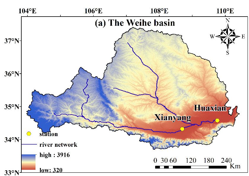
The basic overview of the four stations is shown in Table 1 and Figure 1 below.
The Weihe River Basin originates in Bird Rat mountain in Weiyuan County, Gansu Province,
and flows through Gansu and Shaanxi provinces to the Yellow River in Tongguan County, Weinan City
(Figure 1a). The river is 818 km long, with a basin area of 134,766 km2 and geographical coordinates
at 33◦ 400 –37◦ 260 N and 103◦ 570 –110◦ 270 E [47]. The interannual variation of runoff in the middle
and lower reaches of the Weihe River is characterized by small southern and large northern runoff.
The mainstream flow of the Weihe River is the largest in autumn, accounting for 38% to 40% of annual
runoff, 32.8% to 34.2% in summer, 17.7% to 19.1% in spring, and 8.3% to 9.9% in winter. The rainfall
in the middle and lower reaches of the Weihe River is concentrated in July, August and September,
and there are many heavy rains and flood disasters.
The Pearl River originates in Maxiong Mountain, Qujing City, Yunnan Province, and flows through
Yunnan, Guizhou, Guangxi, Guangdong, Hunan, Jiangxi, and northern Vietnam. It is injected intoWater 2020, 12, 1867 7 of 17
the South Sea from eight downstream estuaries, with a total length of 2320 km and a basin area of
45,369 km2 (Figure 1b). The Pearl River Basin consists of four river systems including Xijiang, Beijiang,
Dongjiang, and the Zhujiang Delta [48]. The average annual rainfall of the basin is 1200–2200 mm,
and the annual runoff is more than 330 billion m3 . The flood season accounts for 80% of the total
annual runoff from April to September, and accounts for more than 50% of the annual runoff in summer
(June–August).
Table 1. The information on the hydrological stations used in this study.
Basin Station Control Basin Area/(km2 ) Longitude Latitude Data Period
Pearl River Gaodao 7007 113.17 24.16 1954–2014
Dahuangjiangkou 288,544 110.20 23.58 1954–2009
Weihe River Xianyang 46,827 108.70 34.32 1954–2011
Huaxian 106,498 109.76 34.58 1951–2012
Water 2020, 12, x FOR PEER REVIEW 8 of 18
Figure 1a
Locationmaps
Figure1.1.Location
Figure mapsof
ofthe
thehydrological
hydrologicalstations
stationsof
of(a)
(a)the
theWeihe
Weihe basin
basin and
and (b)
(b) the
the Pearl
Pearl basin.
basin.
4. Results
4. Results
4.1. Mann–Kendall Trend Analysis
4.1. Mann–Kendall Trend Analysis
A Mann–Kendall test was carried out on the historical data from each station using the trend
packageMann–Kendall
A test From
in the R language. was carried
this, theout
P, |Zon the historical data from each station using the trend
c |, and S values of the Huaxian, Gaodao, Dahuangjiangkou,
package in the R language. From this, the P, |Zc|, and S values of the Huaxian, Gaodao,
Dahuangjiangkou, and Xianyang stations were obtained. The P, |Zc|, and S values of the four stations
are shown in Table 2 below.
Table 2. Results of trend analysis for each station.
Mann–Kendall Test Huaxian Gaodao Dahuangjiangkou XianyangWater 2020, 12, 1867 8 of 17
and Xianyang stations were obtained. The P, |Zc |, and S values of the four stations are shown in
Table 2 below.
Table 2. Results of trend analysis for each station.
Mann–Kendall Test Huaxian Gaodao Dahuangjiangkou Xianyang
P value 2.117 × 10⁻⁵ 3.596 × 10⁻² 5.727 × 10⁻² 3.236 × 10⁻⁴
|Zc | 4.2522 2.0974 1.9013 3.5956
S −701 338 270 −537
The confidence interval was set to 95%, at which Za/2 = 1.96. The trends of Huaxian, Gaodao,
and Xianyang stations were significant at a 5% significance level, while the trend of Dahuangjiangkou
station was significant at a 10% significance level. Moreover, the positive and negative relationships
among the S values allow us to conclude that Gaodao and Dahuangjiangkou stations showed an
increasing trend, while the other stations showed a decreasing trend. Huaxian and Xianyang stations
showed Figure 1a decreasing trend, while Gaodao station showed a significantly increasing trend.
a significantly
Finally, Dahuangjiangkou station showed no significant upward trend. Figure 2 shows the linear trend
line of the annual maximum flood series at each station.
Figure 2. Linear trend line of annual maximum flood series for (a) Huaxian station; (b) Gaodao station;
Figure 2. Linear
(c) Dahuangjiangkou trend(d)
station; line of annual
Xianyang maximum flood series for (a) Huaxian station; (b) Gaodao station;
station.
(c) Dahuangjiangkou station; (d) Xianyang station.Water 2020, 12, 1867 9 of 17
4.2. Determination of Optimal GAMLSS-CB Model
In order to select the optimal probability distribution type, the annual maximum flood series
of four stations in the Weihe River and the Pearl River Basin located in different climate regions of
China was selected as the research object. The time t was the covariate, and the relationship between
the statistical parameters and the covariate was the cubic B-spline function; AIC was the evaluation
criterion, and the gamma distribution (two-parameter), lognormal distribution (two-parameter) and
GEV distribution were compared respectively. The shape parameter of GEV is sensitive and difficult
to estimate; thus, it is assumed to be constant in this study in keeping with other studies [49,50].
The normal QQ graph can be used to judge the performance of the GAMLSS-CB optimal model.
For each station, a total of 12 non-stationary models were constructed considering the combination of
distribution types and variation types for each location and scale parameter. The corresponding AIC
values are shown in Table 3 below.
Table 3. Akaike information criterion (AIC) values of the non-stationary models for each station. Note
that letter “L” in the models’ names represents location parameter and “S” represents scale parameters.
Number “0” means the parameter is invariant while “t” means the parameter varies with time covariate.
Besides, the AIC value in bold is the optimal model for each station.
Models Huaxian Gaodao Dahuangjiangkou Xianyang
GA_L0_S0 1067.70 1061.64 1159.68 969.63
GA_Lt_S0 1054.85 1060.90 1157.02 961.10
GA_L0_St 1070.72 1061.30 1162.43 967.90
GA_Lt_St 1054.82 1062.00 1158.25 960.70
LN_L0_S0 1069.93 1063.52 1161.63 974.87
LN_Lt_S0 1055.30 1065.35 1158.33 962.34
LN_L0_St 1074.37 1062.89 1164.26 972.17
LN_Lt_St 1055.15 1064.75 1159.39 961.94
GEV_L0_S0 1073.05 1063.11 1159.98 974.70
GEV_Lt_S0 1070.33 1068.79 1161.86 972.10
GEV_L0_St 1075.58 1061.00 1158.39 977.23
GEV_Lt_St 1068.71 1064.02 1160.38 975.24
It can be concluded that the gamma distribution is the optimal distribution when using the
GAMLSS-CB model. The non-stationary gamma distribution with both location parameters and scale
parameters changing with time had the best performance for Huaxian and Xianyang stations: the AIC
values were 1054.82 and 960.70. However, for Gaodao and Dahuangjiangkou stations, the optimal
models were non-stationary gamma distribution with location parameters changing with time and the
scale parameters remaining unchanged: the AIC values were 1060.90 and 1157.02. Figure 3 shows the
QQ map of the optimal non-stationary model for each hydrological station. The results show that the
optimal non-stationary model empirical residual and theoretical residual are stationary and distributed
near the 1:1 line, indicating that the model has a good performance.Water 2020, 12, 1867 10 of 17
Figure 3. QQ map of the optimal non-stationary models for (a) Huaxian station; (b) Gaodao station;
Figure 3. QQ map of the optimal non-stationary models for (a) Huaxian station; (b) Gaodao station;
(c) Dahuangjiangkou station; (d) Xianyang station.
(c) Dahuangjiangkou station; (d) Xianyang station.
4.3. Comparison of Model Performance
4.3.1. Qualitative Analysis of Model Performance
Qualitative analysis of the probabilistic coverage rate of models was conducted by calculating the
quantile curve of each station using the QR-L, QR-CB, and GAMLSS-CB models; see the following
Figures 4–6 for details. Table 4 below shows the probabilistic coverage rate of non-stationary models
for each station. It can be concluded that in the QR-L model the probability coverage deviation of the
Huaxian station model was 0.81%–4.84%, the deviation of Gaodao station was 0.08%–5.74%, the deviation
of Dahuangjiangkou station was 0–0.36%, and the deviation of Xianyang station was 0–2.59% (Figure 4).
The QR-CB model shows that the probability coverage deviation of Huaxian station was 0–2.42%,
the deviation of the Gaodao station model was 0.08%–2.87%, the deviation of Dahuangjiangkou station
was 0–1.79%, and the deviation of Xianyang station was 0.17%–5.17% (Figure 5). The GAMLSS-CB model
probability coverage deviation of Huaxian station was 0.16%–10.48%, the deviation of Gaodao station is
0.08%–6.97%, the deviation of Dahuangjiangkou station was 0.36%–5.36%, and the deviation of Xianyang
station was 0.17%–4.31% (Figure 6). Based on the overall data, the performance of the QR-L and QR-CB
models was basically the same, while the performance of the GAMLSS-CB model was slightly weaker.Water 2020, 12, 1867 11 of 17
Table 4. Qualitative analysis of probability coverage of non-stationary models for each station.
Quantile/%
Station Model
5 25 50 75 95
Huaxian QR-L 6.45 24.19 45.16 75.81 93.55
QR-CB 3.23 22.58 50.00 72.58 95.16
GAMLSS-CB 4.84 35.48 46.77 69.35 96.77
Gaodao QR-L 3.28 21.31 44.26 73.77 95.08
QR-CB 4.92 24.59 52.46 72.13 95.08
GAMLSS-CB 4.92 18.03 50.82 77.05 93.44
Dahuangjiangkou QR-L 5.36 25.00 50.00 75.00 96.43
QR-CB 3.57 23.21 50.00 75.00 96.43
GAMLSS-CB 3.57 26.79 44.64 76.79 94.64
Xianyang Station QR-L 5.17 24.14 50.00 72.41 96.55
QR-CB 3.45 22.41 55.17 72.41 94.83
GAMLSS-CB 5.17 29.31 48.28 75.86 94.83
Quantile4.curves
Figure 4. Figure of QR-L
Quantile modelof
curves for QR-L
(a) Huaxian
modelstation; (b) Gaodao
for (a) Huaxianstation; (c) Dahuangjiangkou
station; (b) Gaodao station; (c)
station; (d) Xianyang station.
Dahuangjiangkou station; (d) Xianyang station.Figure 4. Quantile curves of QR-L model for (a) Huaxian station; (b) Gaodao station; (c)
Water 2020, 12, 1867 12 of 17
Dahuangjiangkou station; (d) Xianyang station.
Figure 5. Quantile
Figure curves of QR-CB
5. Quantile model
curves for (a) Huaxian station; (b) Huaxian
Gaodao station; (c)(b)
Dahuangjiangkou
Dahuangjiangkou station; (d)ofXianyang
QR-CB model
station. for (a) station; Gaodao station; (c)
station; (d) Xianyang station.
Quantile
Figure 6. Figure curves ofcurves
6. Quantile GAMLSS-CB model model
of GAMLSS-CB for (a)for
Huaxian station;
(a) Huaxian (b) Gaodao
station; station;
(b) Gaodao station; (c)
(c) Dahuangjiangkou station; (d) Xianyang station.
Dahuangjiangkou station; (d) Xianyang station.Water 2020, 12, 1867 13 of 17
4.3.2. Quantitative Analysis of Model Performance
We quantitatively compared the performance of the model by calculating the Filliben correlation
coefficient. The model Filliben correlation coefficient is shown in Table 5 below. According to the
principle that when the Filleben correlation coefficient is larger, the performance is better, we found
that the performance of each station model was good, especially the GAMLSS-CB model, which had
the best model performance compared with the QR-L and QR-CB models, and that the performance of
the QR-L model was better than the QR-CB model.
Table 5. Filliben correlation coefficient of each station.
Models Huaxian Gaodao Dahuangjiangkou Xianyang
QR-L 0.9831 0.9831 0.9835 0.9830
QR-CB 0.9793 0.9835 0.9715 0.9548
GAMLSS-CB 0.9871 0.9834 0.9913 0.9968
Since the accuracy of qualitative analysis is affected by the rules of artificial counting, and the
accuracy of quantitative analysis is more secure, in this study quantitative analysis was the main
method and qualitative analysis was auxiliary. This study found that the GAMLSS-CB model had the
best model performance compared with the QR-L and QR-CB models, based on qualitative analysis
and quantitative analysis. Then the ADLL method was used to estimate the non-stationary design
flood value of the GAMLSS-CB model.
4.4. Design Values of GAMLSS-CB Model
This study concluded that the GAMLSS-CB model had the best model performance compared
with the QR-L and QR-CB models. Therefore, this study assumed the engineering design period to
be 50 years, from 2015 to 2064, and used the GAMLSS-CB model to estimate the flood design value.
Figure 7 below shows that the flood design values estimated by the ADLL method based on the
GAMLSS-CB model were reasonable and reliable. It can be used for non-stationary engineering design
due to its linkage with the design period of projects under changing environments.
Figure 7. Flood design values estimated by average design life level (ADLL) method based on
Figure 7. Flood design values estimated by average design life level (ADLL) method based on GAMLSS-CB
GAMLSS-CB model for (a) Huaxian station; (b) Gaodao station; (c) Dahuangjiangkou station; (d)
model for (a) Huaxian station; (b) Gaodao station; (c) Dahuangjiangkou station; (d) Xianyang station.
Xianyang station.Water 2020, 12, 1867 14 of 17
5. Discussion
Currently, there are very few studies estimating design flood value based on the quantile regression
model, largely because the design results are affected by the distribution of sample points when
estimating design flood values based on the quantile regression model. The number of available
observations in particular becomes lower when estimating design values corresponding to higher
return periods, leading to unreasonable and inaccurate design values. For this reason, this study
does not compare the design flood values estimated using the quantile regression model with those
using other models. In future studies, more research efforts are needed to improve the accuracy of
design values based on quantile regression. For example, to avoid the influence of rare sample points
of extreme floods when estimating design values with higher return period, we can turn to use the
“peak-over-threshold” (POT) sampling method to increase the sample size of extreme floods. Different
from the annual maximum sampling method of selecting only one sample per year, the sample size
can be expanded by selecting 2–3 high-quantile flood samples exceeding the threshold using the POT
sampling method, thus solving the problem of scarce high-quantile flood samples in estimating design
values based on quantile regression.
The GAMLSS-CB model has a good performance, and its method of estimating design flood
value is stable and reliable. Therefore, the accuracy of the design flood value estimated by the
model is guaranteed, but the currently constructed GAMLSS-CB model only considered time as a
covariate, which has certain limitations. In later research, we should try to add population, climate, etc.
as covariates to optimize the GAMLSS-CB model.
In this study, only the point estimation of design quantiles was presented, which lacks standard
error estimation. Nasri et al. [33] developed the GEV-B-Spline model and evaluated the uncertainties
of design quantiles using the bias (BIAS) and the root mean square error (RMSE). They found that the
Bayesian estimation for the GEV-B-Spline model can achieve satisfactory results. Therefore, in future
research, we will consider using Bayesian estimation or other methods to improve the accuracy of
parameter estimation and explore the uncertainties of design flood values.
6. Conclusions
This paper constructed GAMLSS-CB, QR-CB and QR-L models based on the annual maximum
flood series of four stations in the Weihe River and the Pearl River basin located in different climate
regions of China, and compared the model performance of different non-stationary models using
probability coverage and Filliben correlation coefficient. In addition, the design flood values under
changing environments were also estimated using the optimal model. The main conclusions of this
study are obtained as follows:
(1) Through the Mann–Kendall trend test, it is concluded that both Huaxian station and Xianyang
station showed a significantly decreasing trend, while Gaodao station showed a significantly
increasing trend. In addition, Dahuangjiangkou station showed no significant upward trend.
(2) The gamma distribution is the optimal distribution when using the GAMLSS-CB model.
The non-stationary gamma distribution with both location parameters and scale parameters
changing with time had the best performance for Huaxian and Xianyang stations, while for Gaodao
and Dahuangjiangkou stations the optimal models were non-stationary gamma distribution with
location parameters changing with time and the scale parameters remaining unchanged.
(3) The GAMLSS-CB model showed the best model performance compared with the QR-L and
QR-CB models, based on qualitative and quantitative analysis. When the design flood values are
estimated based on the GAMLSS-CB model using the ADLL method, the design values are not
affected by the distribution of sample points. The non-stationary design flood values estimated
by the ADLL method are reasonable and reliable. It can be used for non-stationary engineering
design due to its linkage with the design period of projects under changing environments.Water 2020, 12, 1867 15 of 17
Author Contributions: Conceptualization, L.Y. and C.Q.; methodology, J.L.; validation, P.Y. and F.C.; formal
analysis, P.Y. and D.L.; investigation, L.Y. and J.L.; data curation, J.L. and D.L.; writing—original draft preparation,
C.Q. and J.L.; writing—review and editing, L.Y.; visualization, J.L. and F.C. All authors have read and agreed to
the published version of the manuscript.
Funding: This research is financially supported jointly by the National Natural Science Foundation of China
(51909053), the Natural Science Foundation of Hebei Province (E2019402076), the Youth Foundation of the
Education Department of Hebei Province (QN2019132), and the Innovation Fund Project of Hebei University of
Engineering (SJ010002123).
Acknowledgments: Great thanks are due to the editor and reviewers for their valuable comments on how to
improve the quality of this paper.
Conflicts of Interest: The authors declare no conflict of interest.
References
1. Gu, X.; Zhang, Q.; Singh, V.P.; Xiao, M.; Cheng, J. Nonstationarity-based evaluation of flood risk in the Pearl
River basin: Changing patterns, causes and implications. Hydrol. Sci. J. 2017, 62, 246–258. [CrossRef]
2. Gu, X.; Zhang, Q.; Singh, V.P.; Song, C.; Sun, P.; Li, J. Potential contributions of climate change and
urbanization to precipitation trends across China at national, regional and local scales. Int. J. Climatol. 2019,
39, 2998–3012. [CrossRef]
3. Hu, Y.; Liang, Z.; Singh, V.P.; Zhang, X.; Wang, J.; Li, B. Concept of equivalent reliability for estimating the
design flood under non-stationary conditions. Water Resour. Manag. 2018, 32, 997–1011. [CrossRef]
4. Liang, Z.; Yang, J.; Hu, Y.; Wang, J.; Li, B.; Zhao, J. A sample reconstruction method based on a modified
reservoir index for flood frequency analysis of non-stationary hydrological series. Stoch. Env. Res. Risk Assess.
2017, 32, 1561–1571. [CrossRef]
5. Li, J.; Lei, Y.; Tan, S.; Bell, C.D.; Engel, B.A.; Wang, Y. Nonstationary flood frequency analysis for annual flood
peak and volume series in both univariate and bivariate domain. Water Resour. Manag. 2018, 32, 4239–4252.
[CrossRef]
6. Li, J.; Zheng, Y.; Wang, Y.; Zhang, T.; Feng, P.; Engel, B.A. Improved mixed distribution model considering
historical extraordinary floods under changing environment. Water 2018, 10, 1016. [CrossRef]
7. Li, J.; Ma, Q.; Tian, Y.; Lei, Y.; Zhang, T.; Feng, P. Flood scaling under nonstationarity in Daqinghe River basin,
China. Nat. Hazards 2019, 98, 675–696. [CrossRef]
8. Salas, J.D.; Obeysekera, J.; Vogel, R.M. Techniques for assessing water infrastructure for nonstationary
extreme events: A review. Hydrol. Sci. J. 2018, 63, 325–352. [CrossRef]
9. Song, X.; Lu, F.; Wang, H.; Xiao, W.; Zhu, K. Penalized maximum likelihood estimators for the nonstationary
Pearson type 3 distribution. J. Hydrol. 2018, 567, 579–589. [CrossRef]
10. Xiong, L.; Yan, L.; Du, T.; Yan, P.; Li, L.; Xu, W. Impacts of Climate Change on Urban Extreme Rainfall and
Drainage Infrastructure Performance: A Case Study in Wuhan City, China. Irrig. Drain. 2019, 68, 152–164.
[CrossRef]
11. Zeng, H.; Feng, P.; Li, X. Reservoir flood routing considering the non-stationarity of flood series in North
China. Water Resour. Manag. 2014, 28, 4273–4287. [CrossRef]
12. Zeng, H.; Sun, X.; Lall, U.; Feng, P. Nonstationary extreme flood/rainfall frequency analysis informed by
large-scale oceanic fields for Xidayang Reservoir in North China. Int. J. Climatol. 2017, 37, 3810–3820.
[CrossRef]
13. Zhang, T.; Wang, Y.; Wang, B.; Tan, S.; Feng, P. Nonstationary flood frequency analysis using univariate and
bivariate time-varying models based on GAMLSS. Water 2018, 10, 819. [CrossRef]
14. Jiang, C.; Xiong, L.; Yan, L.; Dong, J.; Xu, C. Multivariate hydrologic design methods under nonstationary
conditions and application to engineering practice. Hydrol. Earth Syst. Sci. 2019, 23, 1683–1704. [CrossRef]
15. Kang, L.; Jiang, S.; Hu, X.; Li, C. Evaluation of return period and risk in bivariate non-stationary flood
frequency analysis. Water 2019, 11, 79. [CrossRef]
16. Chavez-Demoulin, V.; Davison, A.C.; McNeil, A.J. Estimating Value-at-Risk: A point process approach.
Quant Financ. 2005, 5, 227–234. [CrossRef]
17. Hao, Z.; Singh, V.P. Review of dependence modeling in hydrology and water resources. Prog. Phys. Geogr.
2016, 40, 549–578. [CrossRef]Water 2020, 12, 1867 16 of 17
18. He, Y.; Bárdossy, A.; Brommundt, J. Non-stationary flood frequency analysis in southern Germany.
In Proceedings of the 7th International Conference on HydroScience and Engineering (ICHE 2006),
Philadelphia, PA, USA, 10–13 September 2006.
19. Khalip, M.N.; Ouarda, T.B.M.J.; Ondo, J.-C.; Gachon, P.; Bobée, B. Frequency analysis of a sequence of
dependent and/or non-stationary hydro-meteorological observations: A review. J. Hydrol. 2006, 329, 534–552.
[CrossRef]
20. Villarini, G.; Smith, J.A.; Serinaldi, F.; Bales, J.; Bates, P.D.; Krajewski, W.F. Flood frequency analysis for
nonstationary annual peak records in an urban drainage basin. Adv. Water Resour. 2009, 32, 1255–1266.
[CrossRef]
21. Villarini, G.; Smith, J.A.; Napolitano, F. Nonstationary modeling of a long record of rainfall and temperature
over Rome. Adv. Water Resour. 2010, 33, 1256–1267. [CrossRef]
22. Gao, J. Study on the spatiotemporal characteristics of extreme precipitation in Yalong River Basin based on
GAMLSS model. Water Power 2019, 4, 13–17, 56, (In Chinese with English Abstract).
23. Su, C.; Chen, X. Assessing the effects of reservoirs on extreme flows using nonstationary flood frequency
models with the modified reservoir index as a covariate. Adv. Water Resour. 2019, 124, 29–40. [CrossRef]
24. Yan, L.; Xiong, L.; Ruan, G.; Xu, C.Y.; Yan, P.; Liu, P. Reducing uncertainty of design floods of two-component
mixture distributions by utilizing flood timescale to classify flood types in seasonally snow covered region.
J. Hydrol. 2019, 574, 588–608. [CrossRef]
25. Yan, L.; Li, L.; Yan, P.; He, H.; Li, J.; Lu, D. Nonstationary flood hazard analysis in response to climate change
and population growth. Water 2019, 11, 1811. [CrossRef]
26. Koenker, R.; Bassett, G. Regression quantiles. Econom. Soc. 1978, 46, 33–50. [CrossRef]
27. Barbosa, M.S. Quantile trends in Baltic sea level. Geophys. Res. Lett. 2008, 35, L22704. [CrossRef]
28. Mazvimavi, D. Investigating changes over time of annual rainfall in Zimbabwe. Hydrol. Earth Syst. Sci. 2010,
14, 2671–2679. [CrossRef]
29. Wang, H.; Killick, R.; Fu, X. Distributional change of monthly precipitation due to climate change:
Comprehensive examination of dataset in southeastern United States. Hydrol. Process. 2014, 28, 5212–5219.
[CrossRef]
30. Feng, P.; Shang, S.; Li, X. Temporal variation characteristics of annual precipitation and runoff in Luan River
basin based on quantile regression. J. Hydroelectr. Eng. 2016, 35, 28–36, (In Chinese with English Abstract).
31. Nasri, B.; Bouezmarni, T.; André, S.H.; Ouarda, B.M.J.T. Non-stationary hydrologic frequency analysis using
B-spline quantile regression. J. Hydrol. 2017, 554, 532–544. [CrossRef]
32. Hendricks, W.; Koenker, R. Hierarchical spline models for conditional quantiles and the demand for electricity.
J. Am. Stat. Assoc. 1992, 87, 58–68. [CrossRef]
33. Nasri, B.; Adlouni, E.S.; Ouarda, B.M.J.T. Bayesian estimation for GEV-B-Spline model. Open J. Syst. 2013, 3,
118–128. [CrossRef]
34. Parey, S.; Malek, F.; Laurent, C.; Dacunha-Castelle, D. Trends and climate evolution: Statistical approach for
very high temperatures in France. Clim. Chang. 2007, 81, 331–352. [CrossRef]
35. Parey, S.; Hoang, T.T.H.; Dacunhacastelle, D. Different ways to compute temperature return levels in the
climate change context. Environmetrics 2010, 21, 698–718. [CrossRef]
36. Cooley, D. Return periods and return levels under climate change. In Extremes in a Changing Climate;
AghaKouchak, A., Easterling, D., Hsu, K., Schubert, S., Sorooshian, S., Eds.; Springer: Dordrecht,
The Netherlands, 2013; Volume 65, pp. 97–114.
37. Rootzén, H.; Katz, R.W. Design life level: Quantifying risk in a changing climate. Water Resour. Res. 2013, 49,
5964–5972. [CrossRef]
38. Yan, L.; Xiong, L.; Guo, S.; Xu, C.Y.; Xia, J.; Du, T. Comparison of four nonstationary hydrologic design
methods for changing environment. J. Hydrol. 2017, 551, 132–150. [CrossRef]
39. Yan, L.; Xiong, L.; Liu, D.; Hu, T.; Xu, C.Y. Frequency analysis of nonstationary annual maximum flood series
using the time-varying two-component mixture distribution. Hydrol. Process. 2017, 31, 69–89. [CrossRef]
40. López, R.A.J.; Francés, F. Non-stationary flood frequency analysis in continental Spanish rivers, using climate
and reservoir indices as external covariates. Hydrol. Earth Syst. Sci. 2013, 17, 3189–3203. [CrossRef]
41. Zhang, D.; Lu, F.; Zhou, X.; Chen, F.; Geng, S.; Guo, W. GAMLSS model-based analysis on nonstationarity of
extreme precipitation in Daduhe River Basin. Water Resour. Hydr. Eng. 2016, 47, 12–20. (In Chinese with
English Abstract)Water 2020, 12, 1867 17 of 17
42. Hu, Y.; Liang, Z.; Yang, H.; Chen, D. Study on frequency analysis method of nonstationary observation series
based on trend analysis. J. Hydroelectr. Eng. 2013, 32, 21–24, (In Chinese with English Abstract).
43. Scherer, K. Uniqueness of best parametric interpolation by cubic spline curves. Constr. Approx. 1997, 13,
393–419. [CrossRef]
44. Xiong, L.; Jiang, C.; Du, T. Statistical attribution analysis of the nonstationarity of the annual runoff series of
the Weihe River. Water Sci. Technol. 2014, 70, 939–946. [CrossRef]
45. Rigby, A.R.; Stasinopoulos, D.M. Generalized additive models for location scale and shape. J. R. Stat. Soc.
C-Appl. 2005, 54, 507–554. [CrossRef]
46. Filliben, J.J. The probability plot correlation coefficient test for normality. Technometrics 1975, 17, 111–117.
[CrossRef]
47. He, H.; Zhang, Q.; Zhou, J.; Fei, J.; Xie, X. Coupling climate change with hydrological dynamic in Qinling
Mountains, China. Clim. Chang. 2009, 94, 409–427. [CrossRef]
48. Cui, W.; Chen, J.; Wu, Y.; Wu, Y. An overview of water resources management of the Pearl River.
Water Sci. Technol. 2007, 7, 101–113. [CrossRef]
49. Du, T.; Xiong, L.; Xu, C.; Gippel, C.J.; Guo, S.; Liu, P. Return period and risk analysis of nonstationary
low-flow series under climate change. J. Hydrol. 2015, 527, 234–250. [CrossRef]
50. Myoung-Jin, U.; Yeonjoo, K.; Momcilo, M.; Donald, W. Modeling nonstationary extreme value distributions
with nonlinear functions: An application using multiple precipitation projections for U.S. cities. J. Hydrol.
2017, 552, 396–406.
© 2020 by the authors. Licensee MDPI, Basel, Switzerland. This article is an open access
article distributed under the terms and conditions of the Creative Commons Attribution
(CC BY) license (http://creativecommons.org/licenses/by/4.0/).You can also read