ArchLab: a MATLAB tool for the Thrust Line Analysis of masonry arches** - De Gruyter
←
→
Page content transcription
If your browser does not render page correctly, please read the page content below
Curved and Layer. Struct. 2021; 8:26–35

Research Article

Francesco Marmo*

ArchLab: a MATLAB tool for the Thrust Line Analysis
of masonry arches**
https://doi.org/10.1515/cls-2021-0003                                hidden in a famous anagram, and by Gregory, explicitly
Received Sep 23, 2020; accepted Nov 18, 2020                         stated, that started a series of researches employing the
                                                                     catenary analogy to model the equilibrium of arches by
Abstract: According to Heyman’s safe theorem of the limit
                                                                     means of compressive internal actions that are funicular
analysis of masonry structures, the safety of masonry
                                                                     of the applied loads [11]. Alternative approaches, initiated
arches can be verified by finding at least one line of thrust
                                                                     by La Hire and developed by Coulomb, analyze the equi-
entirely laying within the masonry and in equilibrium with
                                                                     librium of arches by studying collapse mechanisms of a
external loads. If such a solution does exist, two extreme
                                                                     series of voussoirs capable to transfer a limited set of ac-
configurations of the thrust line can be determined, respec-
                                                                     tions [28]. A formal explanation of these approaches was
tively referred to as solutions of minimum and maximum
                                                                     given in two renowned papers by Heyman [25] and Koohar-
thrust.
                                                                     ian [29], where the safe and unsafe theorems of the limit
In this paper it is presented a numerical procedure for de-
                                                                     analysis of masonry structures are presented.
termining both these solutions with reference to masonry
                                                                          Nowadays several computational methods are avail-
arches of general shape, subjected to both vertical and hor-
                                                                     able for the analysis of masonry structures. Some of them
izontal loads. The algorithm takes advantage of a simpli-
                                                                     are based on the Finite Element Method (FEM) and are
fication of the equations underlying the Thrust Network
                                                                     capable to take into account sophisticated material mod-
Analysis. Actually, for the case of planar lines of thrust, the
                                                                     els [3, 32, 33, 47]. However, an appropriate application of
horizontal components of the reference thrusts can be com-
                                                                     FEM based analyses requires an accurate knowledge of the
puted in closed form at each iteration and for any arbitrary
                                                                     value and spatial distribution of mechanical properties of
loading condition. The heights of the points of the thrust
                                                                     materials and support settlements [26, 27], which requires
line are then computed by solving a constrained linear opti-
                                                                     detailed survey techniques, unmotivated for ordinary struc-
mization problem by means of the Dual-Simplex algorithm.
                                                                     tures.
The MATLAB implementation of presented algorithm is de-
                                                                          A interesting alternative is represented by the meth-
scribed in detail and made freely available to interested
                                                                     ods that employ the No-Tension (NT) material model [7, 17],
users (https://bit.ly/3krlVxH). Two numerical examples re-
                                                                     which is characterized by a non-smooth behavior and re-
garding a pointed and a lowered circular arch are presented
                                                                     quires suitable techniques to be successfully employed
in order to show the performance of the method.
                                                                     for the analysis of real structures [8, 18]. Additionally,
Keywords: thrust line, limit analysis, masonry arch                  the NT model is embodied by the hypotheses of previ-
                                                                     ously mentioned limit theorems. Some of their computa-
                                                                     tional implementations include the Thrust Network Anal-
                                                                     ysis (TNA) [11, 12, 34, 36, 44] and the Thrust Surface Anal-
                                                                     ysis (TSA) [20], both based on the safe theorem, or the
                                                                     Rigid Block Analysis [13, 24, 31] and the Discrete Element
1 Introduction
                                                                     Method (DEM) [30, 49], which employ the unsafe theorem.
                                                                     Worth mentioning are recent proposals in which a fracture
The analysis of masonry arches is a classical problem of
                                                                     mechanics-based analytical method with elastic-softening
structural mechanics. It was from the intuitions by Hooke,
                                                                     of masonry is applied to analyse the structural behaviour of
                                                                     arch bridges and show how the arch thrust line is affected
                                                                     by crack formation [1, 2].
*Corresponding Author: Francesco Marmo: Dipartiment of
Structures for Engineering and Architecture, University of Naples
                                                                          Although these methods are all capable to analyze
Federico II, Naples, Italy; Email: f.marmo@unina.it                  structures characterized by complicated geometries [35, 46]
** Paper included in the Special Issue entitled: Shell and Spatial   and by unusual construction techniques [19, 37], specific
Structures: Between New Developments and Historical Aspects

 Open Access. © 2021 F. Marmo, published by De Gruyter.               This work is licensed under the Creative Commons Attribution 4.0 License
ArchLab: a MATLAB tool for the Thrust Line Analysis of masonry arches | 27
tools for the analysis of masonry arches are still of scien- crete implementation of the no-tension membrane model
tific interest [6, 38, 45]. Methods based on the kinematic [21] the TLA represents a discrete version of the funicular
approach are used to determine the collapse of arches un- curve. The specialization to a planar line of thrust simpli-
dergoing spreading of supports [16, 22]. Methods based on fies enormously the solution of the horizontal equilibrium
Heyman principles are employed to compute the minimum equations that are used to compute the horizontal com-
thickness [4, 40] and the later load bearing capacity [5, 14] ponents of thrust. Actually, in the proposed version of the
of arches. method, reference values of horizontal thrust are computed
Interestingly, the thrust line analysis can also be used in closed form at each iteration.
to determine the optimal shape of masonry arches sub- The proposed version of the TLA has been implemented
jected to vertical and horizontal loads [39, 41]. In particular, in a MATLAB code, freely downloadable from https://bit.ly/
Michiels and Adriaenssens [39] compute a unique thrust 3krlVxH. The method is implemented within the function
line by defining its span and height. The determination ArchLab that takes as input a table containing the geomet-
of this thrust line is obtained by iteratively adjusting the ric and loading data of the arch. Also some ready-to-run
horizontal and vertical forces applied to the nodes of the example files are provided together with a plotting function,
thrust line. This thrust line is then mirrored with respect to useful to graphically visualize the solutions.
the vertical axis so that the pair of mirrored thrust lines are After describing the general method, this paper illus-
used to define the profile of the arch, while an iterative pro- trates in detail how each portion of the algorithm has been
cedure minimizes its total volume. The approach proposed implemented in the MATLAB function ArchLab. Results re-
by Nikolic [41], instead, employs an analytical modeling of garding the analysis of a pointed and a lowered arch are
a catenary arch of constant and finite thickness, for which also reported in order to show its performance.
the horizontal thrust is determined. Then a thrust line is
analytically determined for this arch. Nikolic shows that
this thrust line is not coincident with the catenary curve
that defines the axis of the arch because of the altered po-
2 Thrust Line Analysis of masonry
sition of the center of gravity of voissors due to their finite arches
thickness and curvature.
Worth mentioning are the two MATLAB tools A discretized thrust line, or funicular polygon, is repre-
ArchNURBS [15] and FRS_Method [23]. The approach imple- sented in Figure 1. It is described by means of B segments
mented in ArchNURBS is based on a nonuniform rational and N vertices. Being the thrust line an open polygon, it is
B-splines (NURBS) representation of arch geometry. A always B = N − 1.
preliminary isogeometric finite-element elastic analysis of Borrowing the nomenclature from the TNA, segments
the arch is performed in order to determine the structural and vertices that form the funicular polygon are called
response under service loads, provided that the corre- branches and nodes. Branches and nodes are ordered form
sponding thrust line fulfills assumed geometric constraints. left to right; hence, branch b j connects nodes n j and n j+1 ,
Successively a limit analysis based on the safe theorem while branches b j−1 and b j share the same node n j .
by Heyman is carried on by considering equilibrium and The geometry of the thrust line is described by the coor-
yielding conditions of blocks interfaces. These equations dinates xj = (x j , y j ) of nodes, defined in a two-dimensional
and constraints are solved as a linear optimization problem Cartesian reference frame. According to Heyman’s prin-
that maximizes the load multiplier. The method employed ciples, the thrust line is required to be contained within
in FRS_Method, insted, computes the line of thrust by solv- the thickness of the arch, hence the vertical coordinates
ing an optimization problem that looks for the funicular of nodes are required to fulfill the inequalities y j,min and
polygon closest to the geometrical axis of the arch [48]. This y j,max , where y j,min and y j,max are the heights of the arch
means that a unique line of thrust is determined, which intrados and extrados. However, different choices can be
is neither one of the two limit configurations of minimum done when setting y j,min ≤ y j ≤ y j,max , depending on the
or maximum thrust, neither it obeys to the principle of specific needs of the user. For instance they can be set equal
least action. Additionally, the authors employed a new to the thirds of the arch thickness if the limit condition im-
definition of geometric safety factor of the arch, which is plies a fully compressed arch.
alternative to the one given by Heyman. The generic j-th node is loaded by external forces fj =
The objective of this paper is the Thrust Line Analy- (f jx , f jy ), while the first and last nodes are also subjected to
sis (TLA) of masonry arches, a specialization of the TNA the reactions rl and rr of left and right springers of the arch.
to the two-dimensional case. As the TNA represents a dis- Nodes are also subjected to the thrust forces transmitted28 | F. Marmo
Figure 1: A schematic view of the thrust line
by the adjacent branches. In order to model these internal
forces, a thrust value t j is associated to the generic j-th
branch of the thrust line. Since it represents a compressive
force, t j must be positive, i.e. t j > 0, j = 1, ..., B.
Within the TLA framework, the horizontal position of
nodes and the external forces are known. Thrusts asso-
ciated to branches, vertical position of all nodes and the
reactions of springers are unknown. In the spirit of the
Heyman’s safe theorem, these unknowns are computed by Figure 2: Horizontal thrust
employing equilibrium equations only.
The equilibrium of the generic j-th node of the thrust
thrust line are loaded by the thrust forces associated to the
line is
first and last branches, respectively, and by the springers’
tj−1
j + tjj + fj = 0 (1)
reactions rl and rr . Accordingly, the equilibrium equations
where tj−1 j
j and tj are the thrust forces that branches b j−1 and
of these two nodes read
b j transmit to node n j . These forces have modulus equal to t1 tB
the thrust values t j−1 and t j associated to branches b j−1 and rl + (x1 −x2 )+f1 = 0 , rr + (xN −xN−1 )+fN = 0 (4)
ℓ1 ℓB
b j and they have direction parallel to the corresponding
These equations are easily solved for rl and rr as
branches. Thus, they are computed as
xj − xj−1 xj − xj−1 t1 tB
rl = − (x1 − x2 ) − f1 , rr = − (xN − xN−1 ) − fN (5)
tj−1
j = t j−1 = t j−1 , (2) ℓ1 ℓB
|xj − xj−1 | ℓj−1
xj − xj+1 xj − xj+1 Thus, springers’ reactions are easily computed after the
tjj = t j = tj
|xj − xj+1 | ℓj thrust values of all branches and vertical coordinates of all
√︁ nodes are determined. To this end, the set of equilibrium
where ℓj = |xj+1 − xj | = (x j+1 − x j )2 + (y j+1 − y j )2 is the equations associated to internal nodes is solved first.
length of branch b j . In order to simplify this set of equations, it is useful to
Employing previous formulas, equilibrium of node n j introduce the so-called reference thrusts ^t j = R t̄ j . They are
becomes proportional to the horizontal projection t̄ j of t j by means of
t j−1 tj the positive scalar parameter R > 0. Such reference thrusts
(xj − xj−1 ) + (xj − xj+1 ) + fj = 0 (3)
ℓj−1 ℓj are introduced within equation (3) by setting
Two exceptions shall be considered for the generic equi- tj ℓj ℓj ℓj ^t j
= ⇔ tj = t̄ j = (6)
librium equation (3). Actually, the first and last nodes of the t̄ j h j hj hj RArchLab: a MATLAB tool for the Thrust Line Analysis of masonry arches | 29
where h j = x j+1 − x j . Previous equation has been obtained 1 % --- No horizontal forces ---
by invoking the similitude of triangles in Figure 2. 2
3 % Inizialize reference thrusts of branches
Employing previous formula within Eq. (3), the equi- 4 Tref = ones (N -1 ,1)* T0 ;
5
librium of the j-th internal node becomes 6 % Minimum thrust solution ( deepest solution )
7 [ Yd , Rd , Td ]= VertEq (X , Ymin , Ymax , Tref , Fy , -1);
^t j−1 ^t j 8
(x − xj−1 ) + (xj − xj+1 ) + Rfj = 0 (7) 9 % Maximum thrust solution ( shallowest solution )
h j−1 j hj 10 [ Ys , Rs , Ts ]= VertEq (X , Ymin , Ymax , Tref , Fy ,1);
This is the generic element of the set of equations used to
perform the thrust line analysis. Figure 3: Solving procedure in absence of horizontal forces. The
Notice that the set of equations that is obtained by function VertEq is coded as in Figure 4.
writing down (7) for all internal nodes is composed of 2(N −
1) = 2N − 2 equations. The number of unknowns, that is 2.1 Solving procedure for thrust lines
represented by B reference thrusts, N vertical coordinates
subjected to vertical loads
of nodes, and the value of R, exceeds by 2 the number of
available equations. Actually, B + N + 1 = 2N. However, In case all nodes of the thrust line are loaded exclusively
these unknowns are also subjected to a set of inequalities by vertical forces, the determination of the thrust line con-
introduced before, i.e. t j > 0, y j,min ≤ y j ≤ y j,max and R > 0 . figurations of minimum and maximum thrust is relatively
This means that the set of equations and inequalities simple. It is implemented by the few lines of MATLAB code
can admit infinite solutions, one unique solution or even no reported in Figure 3.
solutions. In the first case one is interested in determining In absence of horizontal forces, i.e. when f jx = 0, j =
two extreme thrust line configurations, respectively associ- 1, ..., N, the x component of equation (7) reads
ated to a minimum and maximum value of the horizontal
^t j−1 ^t j
component of thrust at springers. Accordingly, these so- (x − x j−1 ) + (x j − x j+1 ) = 0 (8)
h j−1 j hj
lutions are called solutions of minimum and maximum
thrust. Recall that horizontal components of thrusts are Recalling that h j−1 = x j −x j−1 and h j = x j+1 −x j , the previous
inversely proportional to the parameter R, see, e.g., Eq. (6). equation simplifies to
Hence, these solutions are also associated to a maximum ^t j−1 − ^t j = 0 (9)
and minimum value of R, respectively. Furthermore, these
two solutions correspond to the deepest and shallowest that leads to uniform distribution of reference thrusts in
geometry of the thrust line. Hence, they are also called all branches. Accordingly, all reference thrusts can be set
deepest and shallowest solutions. equal to an arbitrary small positive value ^t0 . This is done
In case the solution is unique, one can imagine that at line 4 in Figure 3.
the interval between the deepest and the shallowest solu- After the reference thrusts are assigned, the algorithm
tions is reduced in such a way that the two extreme cases solves twice the vertical equilibrium equations to compute
coincide. This situation represents a limit condition for the the solutions of minimum and maximum thrusts, respec-
equilibrium of the arch since only one equilibrated distri- tively. This is done by invoking the function VertEq at lines
bution of internal forces is possible. A small modification 7 and 10 of Figure 3. The MATLAB code of this function is
of the arch geometry or a modest alteration of the loading reported in Figure 4.
condition can result in an unsafe structure. The vertical equilibrium of the generic j-th node is ob-
Finally, in case no solution exists, then there is no dis- tained by selecting the y component of equation (7), which
tribution of internal forces that equilibrate applied loads reads
and fulfill the material assumptions. This means that the ^t j−1 ^t j
(y − y j−1 ) + (y j − y j+1 ) + Rf jy = 0 (10)
arch is unsafe. h j−1 j hj
The procedure for solving the set of equations (7), for The set of N −1 vertical equilibrium equations of all internal
j = 2, ..., N − 1, and the corresponding inequalities, is nodes are written in matrix form as
particularly simplified in case all nodal forces are vertical.
Dy + Rfy = 0 (11)
Actually, in this case it is possible to set up a procedure in
which thrusts and vertical coordinates of nodes are uncou- where y is the vector collecting the y coordinates of all
pled. This simpler case is described first, while the more nodes, fy collects the vertical component of the forces ap-
general case of thrust lines subjected to both vertical and plied at nodes n2 ..., n N−1 and D is the N − 2 × N matrix col-
horizontal loads is presented later on. lecting the reference thrust densities ^t j /h j of all branches. It30 | F. Marmo
1 function [y ,R , T ]= VertEq (X , Ymin , Ymax , Tref , Fy , pm )
2 % Solve vertical equilibrium of the thrust line
3 % pm = -1 -> Minimum thrust solution ( deepest solution )
4 % pm = +1 -> Maximum thrust solution ( shallowest solution )
5
6 N = length ( X );
7
8 % Matrix of reference thrust densities
9 D0 = zeros ( N );
10 Db0 =[1 , -1; -1 ,1];
11 for j =1: N -1
12 jj = j : j +1;
13 D0 ( jj , jj )= D0 ( jj , jj )+ Db0 * Tref ( j )/( X ( j +1) - X ( j ));
14 end
15
16 % select internal nodes
17 D = D0 (2: N -1 ,:);
18 fy = Fy (2: N -1);
19
20 % Constrained linear optimization
21 options = optimset ( ’ Display ’ , ’ none ’ , ’ Algorithm ’ , ’ dual - simplex ’ );
22 F =[ zeros (N ,1); pm ];
23 Aeq =[ D , fy ];
24 beq = zeros (N -2 ,1);
25 lb =[ Ymin ;0];
26 ub =[ Ymax ; Inf (1)];
27 [ Sol ,~ , ExitFlag ]= linprog (F ,[] ,[] , Aeq , beq , lb , ub ,[] , options );
28
29 if ExitFlag ==1
30 % Output solution
31 y = Sol (1: end -1);
32 R = Sol ( end );
33 else
34 % No solution found
35 y = - ones (N ,1);
36 R = -1;
37 end
38
39 % Evaluate actual thrusts
40 T = Tref ;
41 for j =1: N -1
42 Th = Tref ( j )/ R ;
43 Tv = Th *( y ( j +1 ,1) - y (j ,1))/( X ( j +1 ,1) - X (j ,1));
44 T ( j )= norm ([ Th , Tv ]);
45 end
Figure 4: MATLAB function VertEq: solution of the vertical equilibrium of a thrust line
is obtained by assembling the contribution of each branch, Notice that the objective function in (13) is either −R or
that is [︃ ]︃ +R, depending whether the optimization problem is used
^t j 1 −1
Dj = (12) to maximize or minimize R. Either one of the two cases is
h j −1 1 selected by setting pm = -1 or pm = +1 to the last input variable
It is assembled in rows j and j + 1 and columns j and j + 1 of VertEq (lines 7 and 10 in Figure 3). Actually, from equation
of D (lines 8 − 18 of Figure 4). (6) it is clear that higher values of R are associated to lower
The unknowns y and R are determined by solving Eq. values of thrust and vice versa. Accordingly, when the ob-
(11) together with the set of inequalities that express the jective function −R is used, the value of R is maximized and
corresponding constrains. Hence, y and R are computed the optimization procedure returns the so-called solution of
by solving the following constrained linear optimization minimum thrust or deepest solution. Similarly, the solution
problem: of maximum thrust or shallowest solution is obtained when
⎧ R is minimized, i.e. when the objective function is set as
⎪
⎪
⎨ Dy + Rf y = 0 +R.
min ±R such that ymin ≤ y ≤ ymax (13)
y, r ⎪
⎪
⎩R > 0
by means of the Dual-Simplex Algorithm [42] already avail-
able in MATLAB. It is invoked at lines 20 − 27 of Figure
4.ArchLab: a MATLAB tool for the Thrust Line Analysis of masonry arches | 31
1 % --- Horizontal forces ---
2
3 % ++ Minimum thrust solution ( deepest solution ) ++
4 Rd =1 e -8;
5 for k =2:100
6
7 % Assign reference thrusts that fulfill horizontal equilibrium
8 Tref = RefThr ( Fx ,N , T0 , Rd );
9
10 % Vertical equilibrium
11 Rold = Rd ;
12 [ Yd , Rd , Td ]= VertEq (X , Ymin , Ymax , Tref , Fy , -1);
13
14 % Check convergence
15 if ( Rd == -1)||( abs ( Rd - Rold )32 | F. Marmo
1 function T = RefThr ( fx ,N , T0 , R ) The function ArchLab takes as input the horizontal
2 % Assign reference thrusts position x of the nodes of the thrust line, their height lim-
3
4 T = ones (N -1 ,1)* T0 ; its, ymin and ymax , and the applied forces, f x and f y . These
5
6 for j =2: N -1 data are included in the two table files PointedArch.csv
7 T ( j )= T (j -1)+ fx ( j )* R ; and LoweredArch.csv, respectively. The geometry and the
8 end
9 loading condition of these arches is determined as a func-
10 if min ( T )ArchLab: a MATLAB tool for the Thrust Line Analysis of masonry arches | 33
Figure 8: Deepest and shallowest solutions for a pointed arch subjected to vertical and horizontal loads
Figure 9: Deepest and shallowest solutions for a lowered arch subjected to vertical and horizontal loads
portional to the vertical ones by a factor λ = f x /f y = 0.15. capability of lowered arches to withstand higher values of
The corresponding solutions of minimum and maximum horizontal forces.
thrust are reported in Figure 8. Within this figure, the val-
ues of the scalar parameter R associated to the deepest and
shallowest solutions are respectively indicated by R d and
R s . The ratio R s /R d = 0.38 is an estimate of the difference
4 Conclusions
between the two solutions. The more this ratio is different
The function ArchLab is used to determine thrust line con-
from unity, the larger is the geometric safety factor of the
figurations of minimum and maximum thrust of masonry
arch.
arches subjected to both vertical and horizontal loads. It
The intrados of the lowered circular arch is described
represents a specialization of the Thrust Network Analysis
by a unique circle of radius D/2 = H/2 + S2 /8H = 1.625
to the case of a planar line of thrust. The implemented al-
m, while its center lies H − D/2 = 0.625 m below the arch
gorithm has been described in full detail in section 2 where
springers. Similarly to the previous case, horizontal forces
a precise reference to the implemented MATLAB code is
are set as proportional to the vertical ones by a factor λ =
also reported. When only vertical loads are applied, the
f x /f y = 0.5. The deepest and shallowest configurations of
algorithm is capable to determine the thrust line configura-
the thrust line are diagrammed in Figure 9. Also in this case,
tions without the need of any recursive method. Conversely,
the even lower value of the ratio R s /R d = 0.18 shows the
when also horizontal loads are applied, the procedure re-34 | F. Marmo
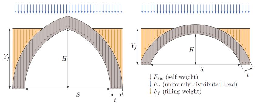
Figure 10: Optimal shape of an arch under its own self-weight and comparison with a catenary curve (dashed)
quires iterations. In both cases, the algorithm computes the [4] Alexakis H, Makris N. Minimum thickness of elliptical masonry
horizontal components of reference thrust in closed form at arches. Acta Mech. 2013;224(12):2977–91.
[5] Alexakis H, Makris N. Limit equilibrium analysis and the mini-
each iteration, while the height of nodes is determined by
mum thickness of circular masonry arches to withstand lateral
solving a constrained linear optimization problem by using
inertial loading. Arch Appl Mech. 2014;84(5):757–72.
the MATLAB builtin implementation of the Dual-Simplex [6] Alexakis H, Makris N. Limit equilibrium analysis of masonry
algorithm. arches. Arch Appl Mech. 2015;85(9-10):1363–81.
By implementing additional few lines of code, not com- [7] Angelillo M, Cardamone L, Fortunato A. A numerical model for
mented in this paper for brevity, it is possible to employ the masonry-like structures. J Mech Mater Struct. 2010;5(4):415–
583.
same functions described earlier to solve a form-finding
[8] Angelillo M, Babilio E, Fortunato A. Singular stress fields from
problem. It is sufficient to set ymin = 0 and ymax = H for all masonry-like vaults. Contin Mech Thermodyn. 2013;25(2-4):423–
nodes of the model and compute the deepest configuration 41.
of the thrust line. Here H represents the arch axis height. An [9] Benvenuto E. Vaulted Structures and Elastic Systems. An intro-
iterative procedure can be used to update the self-weight of duction to the history of structural mechanics. Volume II. NY:
Springer-Verlag. 1991.
each branch of the thrust line and compute updated nodal
[10] Block P, Ciblac T, Ochsendorf J. Real-time limit analysis of vaulted
forces accordingly. An example of such an iterative algo-
masonry buildings. Comput Struc. 2006;84(29-30):551841–52.
rithm is coded within the script ExampleFF, which finds [11] Block P, DeJong M, Ochsendorf J. As hangs the flexible line: equi-
the optimal shape of an arch of span S = 8.0 m and rise librium of masonry arches. Nexus Netw J. 2006;8(2):13–24.
H = 3.0 m, subjected to its own self-weight. The solution is [12] Block P, Ochsendorf J. Thrust network analysis: a new method-
obtained after only 4 iterations and is then plotted by using ology for threedimensional equilibrium. J Int Assoc Shell Spat
Struct. 2007;48:167–73.
the function PlotFF. It is reported in Figure 10, where it is
[13] Cascini L, Gagliardo R, Portioli F. LiABlock_3D: a software tool
compared with the catenary curve y(x) = H + a − Cosh(x/a), for collapse mechanism analysis of historic masonry structures.
with a = 3.0668 m, showing perfect agreement. Int J Archit Herit. 2018;14(1):75–94.
[14] Cavalagli N, Gusella V, Severini L. Lateral loads carrying capacity
Funding information: The author states no funding in- and minimum thickness of circular and pointed masonry arches.
Int J Mech Sci. 2016;115:70645–56.
volved
[15] Chiozzi A, Malagù M, Tralli A, Cazzani A. ArchNURBS: NURBS-
based tool for the structural safety assessment of masonry
Conflict of interest: The author states no conflict of interest arches in MATLAB. J Comput Civ Eng. 2016;30(2):04015010.
[16] Coccia S, Di Carlo F, Rinaldi Z. Collapse displacements for a mech-
anism of spreading-induced supports in a masonry arch. Int. J.
Advanc. Struct. Eng. 2015;7(3):307–20.
References [17] Como M. Statics of historic masonry constructions. 2nd ed. NY:
Springer. 2016.
[1] Accornero F, Lacidogna G. Safety Assessment of Masonry Arch [18] Cuomo M, Ventura G. A complementary energy formulation of no
Bridges Considering the Fracturing Benefit. Appl Sci (Basel). tension masonry-like solids. Comput Methods Appl Mech Eng.
2020;10(10):3490. 2000;189(1):313–39.
[2] Accornero F, Lacidogna G, Carpinteri A. Medieval arch bridges [19] Forgács T, Sarhosis V, Bagi K. Minimum thickness of semi-circular
in the Lanzo Valleys, Italy: incremental structural analysis and skewed masonry arches. Eng Struct. 2017;5140:317–36.
fracturing benefit. J Bridge Eng. 2018;23(7):05018005. [20] Fraddosio A, Lepore N, Piccioni MD. Thrust Surface Method: an
[3] Addessi D, Marfia S, Sacco E, Toti J. Modeling Approaches for innovative approach for the three-dimensional lower bound Limit
Masonry Structures. Open Civ Eng J. 2014;358(1):288–300. Analysis of masonry vaults. Eng Struct. 2020;202:109846.ArchLab: a MATLAB tool for the Thrust Line Analysis of masonry arches | 35
[21] Fraternali F. A thrust network approach for the equilibrium prob- [36] Marmo F, Masi D, Mase D, Rosati L. Thrust network analysis of
lem of unreinforced masonry vaults via polyhedral stress func- masonry vaults. Int J Masonry Research Innovat. 2019;4(1-2):64–
tions. Mech Res Commun. 2010;37(2):198–204. 77.
[22] Galassi S, Misseri G, Rovero L, Tempesta G. Failure modes predic- [37] Marmo F, Ruggieri N, Toraldo F, Rosati L. Historical study and
tion of masonry voussoir arches on moving supports. Eng Struct. static assessment of an innovative vaulting technique of the
2018;173:706–17. 19th century. Int J Archit Herit. 2019;13(6):799–819.
[23] Galassi S, Tempesta G. The Matlab code of the method based on [38] Michiels T, Napolitano R, Adriaenssens S, Glisic B. Comparison
the Full Range Factor for assessing the safety of masonry arches. of thrust line analysis, limit state analysis and distinct element
MethodsX. 2019 Jun;6:1521–42. modeling to predict the collapse load and collapse mechanism
[24] Gilbert M, Melbourne C. Rigid-block analysis of masonry struc- of a rammed earth arch. Eng Struct. 2017;148:145–56.
tures. Struct Eng. 1994;72(21):356–61. [39] Michiels T, Adriaenssens S. Form-finding algorithm for masonry
[25] Heyman J. The stone skeleton. Int J Solids Struct. 1966;2(2):249– arches subjected to in-plane earthquake loading. Comput Struc.
79. 2018;195:85–98.
[26] Heyman J. Structural Analysis, a Historical approach. Cambridge [40] Nikolić D. Thrust line analysis and the minimum thickness of
Univ. Press. 1998. pointed masonry arches. Acta Mech. 2017;228(6):2219–36.
[27] Huerta S. Mechanics of masonry vaults: The equilibrium ap- [41] Nikolić D. Catenary arch of finite thickness as the optimal arch
proach. Historical Constructions. Possibilities of numerical and shape. Struct Multidiscipl Optim. 2019;60(5):1957–66.
experimental techniques. Guimaraes, Portugal: Universidade do [42] Nocedal J, Wright SJ. Numerical Optimization, 2nd ed., Springer
Minho. 2001;47–69. Ser. in Op. Research, Springer-Verlag. 2006.
[28] Huerta S. The Analysis of Masonry Architecture: A Historical Ap- [43] Nodargi NA, Bisegna P. Thrust line analysis revisited and
proach. Archit Sci Rev. 2008;51(4):297–328. applied to optimization of masonry arches, Int J Mech Sci.
[29] Kooharian A. Limit analysis of voussoir (segmental) and concrete 2020;179;105690.
archs. J Am Concr Inst. 1952;24(4):317–28. [44] O’Dwyer D. Funicular analysis of masonry vaults. Comput Struc.
[30] Lemos JV. Discrete element modeling of masonry structures. Int 1999;73(1-5):187–97.
J Archit Herit. 2007;1(2):190–213. [45] Ricci E, Fraddosio A, Piccioni MD, Sacco E. A new numerical ap-
[31] Livesley RK. Limit analysis of structures formed from rigid blocks. proach for determining optimal thrust curves of masonry arches.
Int J Numer Methods Eng. 1978;12(12):1853–71. Eur J Mech A, Solids. 2019;75:426–42.
[32] Lourenco PB, Milani G, Tralli A, Zucchini A. Analysis of masonry [46] Rigó B, Bagi K. Discrete element analysis of stone cantilever
structures: review of and recent trends in homogenization tech- stairs. Meccanica. 2018;53(7):1571–89.
niques. Can J Civ Eng. 2007;34(11):1443–57. [47] Roca P, Cervera M, Gariup G, Pela L. Structural Analysis of
[33] Milani G, Lourenco PB. 3D non-linear behavior of masonry arch Masonry Historical Constructions. Classical and Advanced Ap-
bridges. Comput Struc. 2012;110:133–50. proaches. Arch Comput Methods Eng. 2010;17(3):299–325.
[34] Marmo F, Rosati L. Reformulation and extension of the thrust [48] Tempesta G, Galassi S. Safety evaluation of masonry arches.
network analysis. Comput Struc. 2017;182:104–18. A numerical procedure based on the thrust line closest to the
[35] Marmo F, Masi D, Rosati L. Thrust network analysis of masonry geometrical axis. Int J Mech Sci. 2019;155:206–21.
helical staircases, Int J Arch Her. 502018,12(5):828-848. [49] Tóth AR, Orbán Z, Bagi K. Discrete element analysis of a stone-
masonry arch. Mech Res Commun. 2009;36(4):469–80.You can also read