City-Scale Location Recognition
←
→
Page content transcription
If your browser does not render page correctly, please read the page content below
City-Scale Location Recognition

                       Grant Schindler                           Matthew Brown        Richard Szeliski
                Georgia Institute of Technology                   Microsoft Research, Redmond, WA
                   schindler@cc.gatech.edu                         {brown,szeliski}@microsoft.com

                         Abstract

   We look at the problem of location recognition in a large
image dataset using a vocabulary tree. This entails finding
the location of a query image in a large dataset containing
3 × 10⁴ streetside images of a city. We investigate how the
traditional invariant feature matching approach falls down
as the size of the database grows. In particular we show
that by carefully selecting the vocabulary using the most
informative features, retrieval performance is significantly
improved, allowing us to increase the number of database
images by a factor of 10. We also introduce a generalization
of the traditional vocabulary tree search algorithm which          Figure 1. We perform location recognition on 20 km of urban
improves performance by effectively increasing the branch-         streetside imagery, storing 100 million features in a vocabulary
ing factor of a fixed vocabulary tree.                             tree, the structure of which is determined by the features that are
                                                                   most informative about each location. Shown here is the path of
                                                                   our vehicle over 20 km of urban terrain.

1. Introduction                                                    1.1. Related Work
    The existence of large-scale image databases of the               Vision-based location systems [10, 11, 14] have gener-
world opens up the possibility of recognizing one’s loca-          ally focused on small databases (200-1000 images) taken by
tion by simply taking a photo of the nearest street corner or      human photographers. For example, [10] uses a database of
store-front and finding the most similar image in a database.      200 images, each of a different building facade, and requires
    When this database consists of millions of images of the       manual identification of lines in the database images. We
world, the problem of efficiently searching for a matching         demonstrate results on an automatically captured 30,000
image becomes difficult. The standard approach to image-           image database, consisting of over 100 million SIFT fea-
matching – to convert each image to a set of scale- and            tures [7], and covering a continuous 20 kilometer stretch of
rotation-invariant feature points – runs into storage-space        roads through commercial, residential, and industrial areas.
and search-time problems when dealing with tens of mil-               Searching for images in large databases was the focus
lions of feature points.                                           of [12] and later [9], which used a vocabulary tree of a
    We adopt a vocabulary tree [9] to organize and search          kind described in [2], and earlier in [3], for efficient search.
these millions of feature descriptors without explicitly stor-     In [9], images are documents described by frequencies of
ing the descriptors themselves, a method previously used in        visual words in a latent semantic analysis (LSA) frame-
object recognition. Using vocabulary trees in the context          work, where visual words are defined by both leaf-nodes
of location recognition allows us to determine which fea-          and higher-level nodes in the tree, in a hierarchical fash-
tures are the most informative about a given location and to       ion. We use the same basic data structure of [9], but in
structure the tree based on these informative features. We         several fundamentally different ways. We use neither LSA,
also present a generalization of the traditional search algo-      nor hierarchical scoring, and we focus on building trees for
rithm for vocabulary trees that allows us to improve the per-      specific databases to be used for location recognition, rather
formance of the vocabulary tree at search time as well as          than generic trees for object recognition.
during construction of the tree.                                      The idea of choosing a reduced set of informative fea-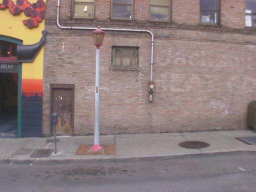
Figure 2. Vocabulary Trees of Varying Branching Factor and Depth. For branching factor k and depth L, we can produce seven trees with
kL ≈ 1, 000, 000 leaf nodes. Starting from top left, the trees are of size 220 , 410 , 106 , 165 , 324 , 1003 , and 10002 . These nested Voronoi
diagrams show each tree projected onto two random dimensions of the 128-dimensional SIFT space. Gray values indicate the ratio of the
distances to the nearest and second-nearest node at each level of the tree (black=1).

tures [13, 6] has previously been used in location and object              there are k L leaf nodes, or visual words, at the bottom of
recognition tasks. We show how to exploit the natural struc-               the tree. It is best understood as the product of a hierarchical
ture of vocabulary trees to define a feature’s information. In             k-means clustering of a number of descriptors, where each
contrast to previous work, rather than reducing the size of                node in the tree is a feature descriptor equal to the mean of
the feature database, we propose using feature information                 all the descriptors assigned to it. The tree is queried by com-
to guide the building of the vocabulary tree instead. The set              paring a query SIFT feature to all k nodes at the root level
of features stored in the leaf nodes of the resulting vocabu-              to find the closest match, and then recursively comparing it
lary tree remains the same. See [5] for a similar approach,                to all k children of that node. The database features corre-
using information loss minimization to build nearest neigh-                sponding to any visual word will all cluster around a single
bor quantizers for use as codebooks in bag-of-features im-                 feature descriptor, and thus we can throw away the SIFT de-
age classification.                                                        scriptor for all features in the database and instead store a
                                                                           6-byte pointer to each feature in the form of an image num-
2. Vocabulary Trees                                                        ber (4-byte int) and feature number (2-byte short).
                                                                               Note that the vocabulary tree is an instance of a metric
   The vocabulary tree [9] is an effective data structure for              tree in the sense used by [8] to distinguish between two
searching a large database in high-dimensional spaces. As                  classes of tree-based data structures: trees which organize
image databases increase in size, we run into several bar-                 data in a vector space in which individual dimensions must
riers that prevent traditional feature matching techniques                 be accessed (e.g. kd-trees), and trees which organize data in
from scaling up. For example, we may have too many                         a metric space in which a metric distance between any two
feature descriptors to store in memory (30,000 images ≈                    points can be computed. In querying a vocabulary tree, we
100,000,000 SIFT features ≈ 12 GB) and far too many fea-                   only ever care about the distance between a query feature
tures to exhaustively compare against a query feature. Even                and each node in the tree. Thus, the structure of the vocab-
kd-trees fail to solve the storage problem since approximate               ulary tree in the 128-dimensional SIFT space can be visu-
k-nearest neighbor algorithms like Best Bin First [1] require              alized as a nested set of Voronoi cells as in Figure 2. Trees
access to feature descriptors at search time. The vocabulary               are constructed with hierarchical k-means as described in
tree solves this storage problem by throwing away the de-                  [9], where we use Gonzalez’s algorithm [4] to initialize the
scriptor for each database feature.                                        cluster centers with points that are as far apart from each
   A vocabulary tree is a k-way tree of depth L such that                  other as possible.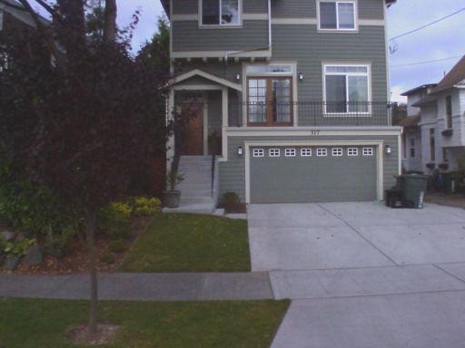
(a) N=1                            (b) N=2                            (c) N=5                           (d) N=9
Figure 3. Greedy N-Best Paths Search. From left to right, we increase the number of nodes N whose children are considered at each level
of the tree. Cells are colored from red to green according to the depth at which they are encountered in the tree, while gray cells are never
searched. By considering more nodes in the tree, recognition performance is improved at a computational cost that varies with N .

3. Greedy N-Best Paths Search                                            Algorithm 1 Greedy N-Best Paths
                                                                         Given query feature q, and level ` = 1
    A popular search heuristic for approximate nearest
                                                                         Compute distance from q to all k children of root node
neighbors in kd-trees is the Best Bin First (BBF) algorithm
                                                                         While (` < L){
[1]. Bounds are computed on the nearest possible feature
                                                                            `=`+1
residing in each path not followed as the search descends
                                                                            Candidates=children of closest N nodes at level ` − 1
down the tree, and a specified number of candidate features
                                                                            Compute distance from q to all kN candidates
are considered in succession. We propose an algorithm sim-
                                                                         }
ilar in spirit to BBF which exploits the unique properties of
                                                                         Return all features quantized under closest candidate
metric trees to allow us to specify how much computation
takes place during nearest neighbor search. We propose the
Greedy N-Best Paths (GNP) algorithm, which follows mul-
                                                                         more nodes are being considered in traversing a tree with
tiple branches at each level rather than just the branch whose
                                                                         higher branching factor. As an example, using a 1 mil-
parent is closest to the query feature. This generalization of
                                                                         lion word vocabulary, consider that in a 106 tree only 60
the traditional vocabulary tree search method is described
                                                                         nodes are ever examined while in a 10002 tree 2000 nodes
in Algorithm 1.
                                                                         are considered during a traditional search. The GNP algo-
    For branching factor k and depth L, the normal search al-
                                                                         rithm offers a way to consider 2010 nodes in a 106 tree with
gorithm for a metric tree performs k comparisons between
                                                                         N = 40, and we show in Section 6 that comparable perfor-
the query feature and the nodes of the tree at each of L lev-
                                                                         mance is achieved with GNP on a tree with fewer branches.
els for a total of kL comparisons. Our algorithm performs
                                                                             Note that changing the branching factor of a vocabulary
k comparisons at the top level, and kN comparisons at each
                                                                         tree requires time-consuming offline re-training via hierar-
of the remaining L − 1 levels, for a total of k + kN (L − 1)
                                                                         chical k-means. However, varying the number of nodes
comparisons. This allows us to specify the amount of com-
                                                                         searched is a decision that can be made at search time based
putation per search by varying the number of paths followed
                                                                         on available computational power. Thus, we should con-
N . Note that traditional search is just the specific case in
                                                                         centrate not on the relationship between performance and
which N = 1.
                                                                         branching factor, but between performance and number of
3.1. Branching Factor                                                    comparisons per query feature, a measure which GNP al-
                                                                         lows us to optimize (see Figure 6).
   For a fixed vocabulary size M , corresponding to the
number of leaf nodes in a tree, there are several ways to                4. Informative Features
construct a vocabulary tree. This is accomplished by vary-
ing the branching factor k and depth L of the tree such that                One of the goals of [9] was to show that acceptable
k L ≈ M for integer values of k and L. In previous work on               recognition performance is possible using a generic vocab-
vocabulary trees[9], it was noted that increasing the branch-            ulary tree trained on data unrelated to the images eventu-
ing factor for fixed vocabulary size tended to improve the               ally used to fill the database. This is important when the
quality of search results. We claim that much of this im-                database is expected to change on the fly. However, if the
provement is due not to the fact that increasing branching               database consists of a fixed set of images, we should instead
factor produces better-structured trees, but to the fact that            aim to build the vocabulary tree which maximizes perfor-
mance of queries on the database.
   For a fixed vocabulary of 1 million visual words, we can
not only vary the branching factor and depth of the tree, but
also choose training data such that the capacity of the tree is                                 0

spent modeling the parts of SIFT space occupied by those                                    −0.01

                                                                              information
features which are most informative about the locations of
the database images. This becomes even more important                                       −0.02

when the database becomes so large that the hierarchical                                    −0.03
k-means process used to build the vocabulary tree cannot
                                                                                                    10                                                             20
possibly cluster all the data at once, but must instead build a                                           8                                               15
tree based on some subset of the database. In selecting the                                                      6
                                                                                                                                                  10
                                                                                                                       4
subset of data for training, we can either uniformly sample                                                                  2             5

the database, or choose those features which are most infor-                                             a = # word at location
                                                                                                                                  0
                                                                                                                                      b = # word not at location
mative, which we explain here.
                                                                   Figure 4. Information gain measures how informative a visual
                                                                   word is about a specific location `i , and it is computed as a func-
4.1. Information Gain                                              tion of a and b, the number of occurrences of a visual word at lo-
    The images in our database contain considerable overlap,       cation `i and at all other locations, respectively. The graph shows
such that we end up with a number of images of each loca-          that information gain is maximized when a visual word occurs of-
                                                                   ten at the location `i and rarely at any other location.
tion from slightly different viewpoints (see Figure 8). Intu-
itively, we want to find features which occur in all images of
some specific location, but rarely or never occur anywhere             We can calculate this conditional entropy H(Li |Wj ) as a
outside of that single location. This intuitive concept is cap-    function of just four terms: NDB , NL , NWj Li , and NWj Li .
tured well by the formal concept of information gain.              The first two terms are constant for a given database: NDB
    Information gain I(X|Y ) is a measure of how much un-          is the number of images in the database, and NL is the num-
certainty is removed from a distribution given some specific       ber of images at each location. The last two terms vary
additional knowledge, and it is defined with respect to the        with each location and visual word: NWj Li is the number
entropy H(X) and conditional entropy H(X|Y ) of distri-            of times visual word wj occurs at location `i , and NWj Li is
butions P (X) and P (X|Y ). By definition:                         the number of times visual word wj occurs at other database
                      X                                            locations. For clarity, we substitute the variables a and b for
         H(X) = −         P (X = x) log[P (X = x)]          (1)    NWj Li and NWj Li in what follows. Note that H(Li |Wj )
                       x                                           depends upon just six probabilities whose values follow
                       X                                           trivially from the definitions of NDB , NL , a, and b:
         H(X|Y ) =             P (Y = y)H(X|Y = y)          (2)
                           y                                                        a                                                       NL − a
                                                                     P (Li |Wj ) =                                          P (Li |Wj ) =
               I(X|Y ) = H(X) − H(X|Y )                     (3)                    a+b                                                    NDB − a − b
                                                                                    b                                                     NDB − NL − b
   In our case, information gain I(Li |Wj ) is always com-           P (Li |Wj ) =                                          P (Li |Wj ) =
                                                                                   a+b                                                     NDB − a − b
puted with respect to a specific location `i and a specific                        a+b                                                  NDB − a − b
visual word wj . Li is a binary variable that is true when              P (Wj ) =                                           P (Wj ) =
                                                                                   NDB                                                     NDB
we are at location `i , and Wj is a binary variable that is true
when the visual word wj is in view (i.e., one of the images at     Substituting these probabilities into Equation 2 above, we
location `i contains a feature which falls under visual word       arrive at the conditional entropy
wj when quantized according to the vocabulary tree). Thus,
                                                                          H(Li |Wj ) =
the information gain of visual word wj at location `i , as
defined in Equation 3, is:                                                  a+b a             a       b          b
                                                                          −      [     log(      )+       log(     )]
                                                                            NDB a + b       a+b     a+b        a+b
             I(Li |Wj ) = H(Li ) − H(Li |Wj )               (4)             NDB − a − b      NL − a           NL − a
                                                                          −             [             log(             )
                                                                                NDB       NDB − a − b      NDB − a − b
Remember that we are interested in finding those visual
                                                                            NDB − NL − b        NDB − NL − b
words at location `i that maximize this information gain                  +                log(               )]      (5)
                                                                             NDB − a − b         NDB − a − b
value. Since the entropy H(Li ) is constant across all vi-
sual words at location `i , then according to Equation 4, the      The significance of this equation is that the information gain
visual word that maximizes the information gain I(Li |Wj )         of a visual word is captured by a simple function of the
also minimizes the conditional entropy H(Li |Wj ).                 values a and b as shown in Figure 4.
0.75
   Note that for a given location, we only need to compute                                                                                                                        info−gain
                                                                                                                                                                                  uniform
                                                                                                                           0.7
this conditional entropy for visual words which actually oc-
                                                                                                                          0.65
cur in the images at that location. In theory, it is possible

                                                                         Performance (% Best Match at Correct Location)
                                                                                                                           0.6
that there may exist some visual word which occurs at every
                                                                                                                          0.55
location except one, in which case this visual word which
                                                                                                                           0.5
does not occur at the given location is nevertheless very in-
formative about that location. In practice, we assume no                                                                  0.45

such features exist, which is supported by the observation                                                                 0.4

that each visual word generally occurs in some small frac-                                                                0.35

tion of the images. Thus, for visual words not present at                                                                  0.3

some location the conditional entropy H(Li |Wj ) ≈ H(Li )                                                                 0.25
                                                                                                                                 5000   10000       15000         20000
                                                                                                                                                # Images in Database
                                                                                                                                                                          25000   30000

and the information gain I(Li |Wj ) ≈ H(Li )−H(Li ) ≈ 0,
                                                                   Figure 5. By building a tree using only the most informative fea-
meaning that for any location there is negligible informa-
                                                                   tures in each database image, we are able to improve performance
tion gain associated with visual words which do not appear
                                                                   over a tree built with training data uniformly sampled from the
there.                                                             database. In all figures, performance is defined as the percentage
   Since the above definition of information gain depends          of query images for which the top match in the database is within
upon having already clustered the data into visual words,          10 meters of the ground truth location of the image.
we bootstrap the process by constructing a number of vo-
cabulary trees for relatively small subsets of the data. We
define information with respect to these smaller subsets, se-      efficiently compute the sums in time linear in the number of
lect the most informative features from each image, and fi-        features Nq in the query image.
nally construct a tree using only these informative features.
                                                                   6. Results
5. Voting Scheme
                                                                       We have a database of 10 million images automatically
    To find the best-matching database image for a given           acquired by driving a vehicle through a large city. Each im-
query image, we match each feature in the query image to a         age measures 1024x768 pixels and has an associated GPS
number of features in the database using a vocabulary tree.        coordinate (latitude and longitude), and a compass heading.
We use a simple voting scheme in which matched features            In these experiments we use a 30,000 image subset cor-
from the database vote for the images from which they orig-        responding to 20 kilometers of streetside data as depicted
inate. To achieve better performance, we normalize the vote        in Figure 1. We evaluate the performance of our location
tallies by Ni (the number of features in a given database im-      recognition method using a set of 278 query images ac-
age i) and N Nk (the number of near neighbors returned for         quired more than one year after the image database. All
a given query feature fk ). In addition, we average the tallies    query images were captured with a 3.2 mega-pixel handheld
over a local neighborhood of NL images. Thus, the num-             consumer digital camera and labeled by hand with the lati-
ber of votes Cd for a database image d can be computed by          tude and longitude of the capture location. In these exper-
looping over every feature in each image in a local neigh-         iments, performance is defined as the percentage of query
borhood, and comparing it against each of the Nq features in       images for which the top match in the database is within 10
the query image, producing the following triple-summation:         meters of the ground truth location of the image.
                     NL                                                We perform two separate experiments – one to evaluate
         1       X2
                d+
                           1 X
                               Ni X
                                  Nq
                                                        1          the effectiveness of using informative features to build vo-
   Cd =                              δmatch (fj , fk )             cabulary trees and the other to evaluate the performance of
        NL            NL
                           Ni j=1                      NNk
               i=d−               k=1
                       2                                           the Greedy N-Best Paths algorithm for vocabulary trees of
where δmatch (fj , fk ) = 1 when database feature fj and           varying branching factor. In the first experiment, we use
query feature fk are both quantized to the same visual word        a one million word vocabulary tree with branching factor
in the vocabulary tree, and δmatch (fj , fk ) = 0 otherwise.       k = 10 and depth L = 6 and the tree is searched using GNP
The number of near neighbors returned for each query fea-          with N = 50 paths. We build two different types of trees
ture fk can be similarly computed as:                              – one is built by hierarchically clustering features sampled
                                                                   uniformly from the database images, while the other is built
                           X
                           NDB X
                               Ni                                  by hierarchically clustering only the most informative fea-
              N Nk =                 δmatch (fj , fk )       (6)   tures in the database. In both cases, a constant 7.5 million
                           i=1 j=1                                 points are used in building the tree as we gradually increase
In practice, we do not explicitly perform these computa-           the size of the database from 3000 images to 30,000 images,
tions for every image, instead using the vocabulary tree to        training new trees for each size of database. The entire 3000
0.75 0.85
0.7 0.8
Performance (% Top Matches at Correct Location)
Performance (% Best Match at Correct Location)
0.65 0.75
0.6 0.7
1000 2
100 3
0.55 0.65
32 4
16 5
10 6
Top 10
0.5 4 10 0.6 Top 5
2 20 Top 3
kd−tree Top 2
Top 1
0.45 0.55
0 1000 2000 3000 4000 5000 0 1000 2000 3000 4000 5000
Comparisons/Query Feature Comparisons/Query Feature
Figure 6. Vocabulary trees of any depth and branching factor can Figure 7. As we consider more than just the best matching result
achieve comparable performance using GNP search. While vocab- for the each of the 278 query images, the percentage of results
ulary trees perform below comparable kd-trees using traditional within 10 meters of the ground truth location increases above 80%.
N = 1 search, they can match and even exceed the performance- These results show the performance of a 324 vocabulary tree on a
per-computation of kd-trees by using GNP search with increasing 3000 image database using GNP with varying N .
values of N . For each query feature, the number of comparisons
against nodes in a vocabulary tree is equal to k + kN (L − 1),
which varies with N the number of best paths searched using the extraction) using a 324 tree and searching with 4-best paths.
GNP algorithm. For the kd-tree, the number of comparisons per
feature is the number of bins considered in the BBF algorithm.
In addition, in Figure 6 we compare the performance
of these vocabulary trees against traditional kd-tree search.
Because kd-trees using the Best-Bin First algorithm access
image database consists of only 7.5 million features, and so the descriptors of every searched database feature, while
both trees are identical at the beginning. As illustrated in vocabulary trees throw away this information, it is tempt-
Figure 5, as images are added to the database, the perfor- ing to think that a kd-tree will naturally perform better at
mance drops for both types of trees. However, the tree built location recognition tasks and that one must compromise
from informative features degrades much more slowly than performance when using vocabulary trees. Just as GNP can
in the uniformly sampled case. be used to vary the amount of computation in a vocabu-
This result is significant because it suggests that the per- lary tree search, the BBF algorithm can consider varying
formance of a vocabulary tree is largely dependent upon numbers of database features. If we equate the number of
its structure. Note that in both trees, the contents of the bins searched in the kd-tree with the number of nodes con-
database are exactly the same, so that the only difference sidered in the vocabulary tree, then we can directly com-
between the two trees is in the way they organize these pare the performance-per-computation of the two types of
database features into visual words. This result tells us that trees. While it is true that vocabulary trees using tradi-
we would not want to use the same generic vocabulary tree tional N = 1 search perform below kd-trees that perform
to perform location recognition in two distinct cities, but the same amount of computation, Figure 6 shows that vo-
rather that we should train such trees separately. This runs cabulary trees can match and even exceed the performance-
counter to the conclusion reached in [9] that generic vocab- per-computation of kd-trees by using GNP search with in-
ulary trees can be used as long as their leaf-nodes are filled creasing values of N .
with new data for each situation. Finally, with respect to the overall performance results,
In the second experiment, we built trees of varying note that in the time between the collection of the database
branching factor and depth as in Figure 2, all with approx- and query images, many elements of the city had changed –
imately one million leaf nodes. We consider a database businesses had hung up new signs and residences had been
of 3000 images and compare the performance of each tree re-modeled, among many other changes, both major and
against the set of 278 query images using the GNP search minor. In addition, much of the query data was taken in poor
algorithm with varying values for N , the number of paths lighting, leading to blurry and low-contrast images which
searched. As discussed in Section 3.1, we can see from more accurately reflect the quality of images one might ex-
Figure 6 that performance varies with the number of nodes pect from an average person unsure of their location. Under
searched more strongly than with the branching factor of these circumstances, the greater than 70% recognition rate
the tree. Though query time varies directly with the con- we achieved exceeded our expectations. Figure 7 also sug-
trollable number of nodes visited in the search, these ex- gests that by employing a geometric consistency check on
periments show that we can achieve close to maximum per- the top 10 matches, we could achieve performance of more
formance in only 0.2 seconds per query (excluding feature than 80%.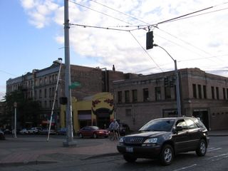
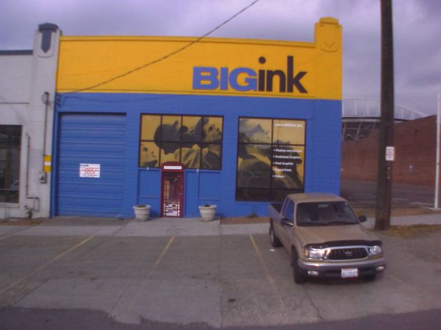
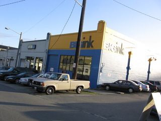
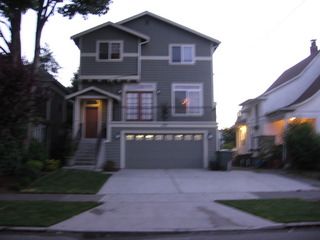
Figure 8. Example database image sequences from commercial (top), residential (middle), and green (bottom) areas of a city. The signifi-
cant overlap between consecutive images allows us to determine which features are most informative about each location.

                                                                       References
                                                                        [1] J. Beis and D. Lowe. Shape indexing using approximate
                                                                            nearest-neighbor search in highdimensional spaces. In IEEE
                                                                            Computer Society Conference on Computer Vision and Pat-
                                                                            tern Recognition, 1997.
                                                                        [2] Sergey Brin. Near neighbor search in large metric spaces. In
                                                                            Int. Conf. on Very Large Data Bases, pages 574–584, 1995.
                                                                        [3] Keinosuke Fukunaga and Patrenahalli M. Narendra. A
                                                                            branch and bound algorithms for computing k-nearest neigh-
                                                                            bors. IEEE Trans. Computers, 24(7):750–753, 1975.
                                                                        [4] T. F. Gonzalez. Clustering to minimize the maximum inter-
                                                                            cluster distance. Journal of Theoretical Computer Science,
                                                                            38(2-3):293–306, June 1985.
                                                                        [5] S. Lazebnik and M. Raginsky. Learning nearest-neighbor
                                                                            quantizers from labeled data by information loss minimiza-
                                                                            tion. In International Conference on Artificial Intelligence
                                                                            and Statistics, 2007.
                                                                        [6] F. Li and J. Kosecka. Probabilistic location recognition using
                                                                            reduced feature set. In IEEE International Conference on
                                                                            Robotics and Automation, 2006.
                                                                        [7] David G. Lowe. Object recognition from local scale-
                                                                            invariant features. In Proc. of the International Conference
Figure 9. Typical examples of the 278 query images (left) and the           on Computer Vision ICCV, Corfu, pages 1150–1157, 1999.
corresponding top matches returned from the database (right) us-        [8] Andrew W. Moore. The anchors hierarchy: Using the trian-
ing a 10002 vocabulary tree with N = 4.                                     gle inequality to survive high dimensional data. In Conf. on
                                                                            Uncertainty in Artificial Intelligence, pages 397–405, 2000.
                                                                        [9] David Nister and Henrik Stewenius. Scalable recognition
                                                                            with a vocabulary tree. In IEEE Computer Society Confer-
                                                                            ence on Computer Vision and Pattern Recognition, 2006.
7. Conclusion
                                                                       [10] Duncan Robertson and Roberto Cipolla. An image-based
                                                                            system for urban navigation. In BMVC, 2004.
   In addition to demonstrating a system for large-scale lo-           [11] Hao Shao, Tomás Svoboda, Tinne Tuytelaars, and Luc J. Van
cation recognition, we have shown two new results with re-                  Gool. Hpat indexing for fast object/scene recognition based
spect to vocabulary trees. First, we have found that the per-               on local appearance. In CIVR, pages 71–80, 2003.
formance of a vocabulary tree on recognition tasks can be              [12] J. Sivic and A. Zisserman. Video google: A text retrieval ap-
significantly affected by the specific vocabulary chosen. In                proach to object matching in videos. In ICCV, pages 1470–
particular, using the features that are most informative about              1477, 2003.
specific locations to build the vocabulary tree can greatly            [13] M. Vidal-Naquet and S. Ullman. Object recognition with
improve performance results as the database increases in                    informative features and linear classification. ICCV, 2003.
size. Second, we have shown that one can improve the
                                                                       [14] W. Zhang and J. Kosecka. Image based localization in ur-
performance of a given vocabulary tree by controlling the
                                                                            ban environments. In International Symposium on 3D Data
number of nodes considered during search, rather than by
                                                                            Processing, Visualization and Transmission, 2006.
increasing the branching factor of the vocabulary tree.
You can also read