Automated Scene Matching in Movies
←
→
Page content transcription
If your browser does not render page correctly, please read the page content below

Automated Scene Matching in Movies

                                  F. Schaffalitzky and A. Zisserman
                                       Robotics Research Group
                                   Department of Engineering Science
                                          University of Oxford
                                           Oxford, OX1 3PJ
                                        fsm,az @robots.ox.ac.uk


       Abstract. We describe progress in matching shots which are images of the same 3D scene
       in a film. The problem is hard because the camera viewpoint may change substantially
       between shots, with consequent changes in the imaged appearance of the scene due to
       foreshortening, scale changes and partial occlusion.
       We demonstrate that wide baseline matching techniques can be successfully employed for
       this task by matching key frames between shots. The wide baseline method represents each
       frame by a set of viewpoint invariant local feature vectors. The local spatial support of the
       features means that segmentation of the frame (e.g. into foreground/background) is not
       required, and partial occlusion is tolerated.
       Results of matching shots for a number of different scene types are illustrated on a com-
       mercial film.

1 Introduction
Our objective is to identify the same rigid object or 3D scene in different shots of a film. This
is to enable intelligent navigation through a film [2, 4] where a viewer can choose to move from
shot to shot of the same 3D scene, for example to be able to view all the shots which take place
inside the casino in ‘Casablanca’. This requires that the video be parsed into shots and that the
3D scenes depicted in these shots be matched throughout the film.
     There has been considerable success in the Computer Vision literature in automatically com-
puting matches between images of the same 3D scene for nearby viewpoints [18, 21]. The meth-
ods are based on robust estimation of geometric multi-view relationships such as planar homo-
graphies and epipolar/trifocal geometry (see [3] for a review).
     The difficulty here is that between different shots of the same 3D scene, camera viewpoints
and image scales may differ widely. This is illustrated in figure 1. For such cases a plethora
of so called “wide baseline” methods have been developed, and this is still an area of active
research [1, 7–9, 11–15, 17, 19, 20].
     Here we demonstrate that 3D scene based shot matching can be achieved by applying
wide baseline techniques to key frames. A film is partitioned into shots using standard meth-
ods (colour histograms and motion compensated cross-correlation [5]). Invariant descriptors are
computed for individual key frames within the shots (section 2). These descriptors are then
matched between key frames using a set of progressively stronger multiview constraints (sec-
tion 3). The method is demonstrated on a selection of shots from the feature film ‘Run Lola Run’
(Lola Rent).
2 Invariant descriptors for multiview matching
In this section we describe the invariant descriptors which facilitate multiple view matches, i.e.
point correspondences over multiple images.
Fig. 1. These three images are acquired at the same 3D scene but from very different viewpoints. The
affine distortion between the imaged sides of the tower is evident, as is the difference in brightness. There
is considerable foreground occlusion of the church, plus image rotation . . .

    We follow the, now standard, approach in the wide baseline literature and start from features
from which we can compute viewpoint invariant descriptors. The viewpoint transformations we
consider are an affine geometric transformation (which models viewpoint change locally) and
an affine photometric transformation (which models lighting change locally). The descriptors
are constructed to be unaffected by these classes of geometric and photometric transformation;
this is the meaning of invariance.
    Features are determined in two stages: first, image regions which transform covariantly with
viewpoint are detected in each frame, second, a vector of invariant descriptors is computed for
each region. The invariant vector is a label for that region, and will be used as an index into
an indexing structure for matching between frames — the corresponding region in other frames
will (ideally) have an identical vector.
    We use two types of features: one based on interest point neighbourhoods, the other based on
the “Maximally Stable Extremal” (MSE) regions of Matas et al. [8]. In both types an elliptical
image region is used to compute the invariant descriptor. Both features are described in more
detail below. It is necessary to have (at least) two types of feature because in some imaged scenes
one particular type of feature may not occur. The interest point features are a generalization of
the descriptors of Schmid and Mohr [16] (which are invariant only to image rotation).
Invariant interest point neighbourhoods: Interest points are computed in each frame, and a
characteristic scale associated with each point using the method of [10], necessary to handle
scale changes between the views. For each point we then compute an affine invariant neighbour-
hood using the adaptive method, proposed by Baumberg [1], which is based on isotropy of the
gradient second moment matrix [6]. If successful, the output is an image point with an ellipti-
cal neighbourhood which transforms co-variantly with viewpoint. Figure 2 shows an example.
Similar neighbourhoods have been developed by Mikolajczyk and Schmid [11].
    For a      pixel video frame the number of neighbourhoods computed is typically
1600, but the number depends of course on the visual richness of the image. The computation
of the neighbourhood generally succeeds at points where there is signal variation in more than
one direction (e.g. near “blobs” or “corners”).
MSE regions: The regions are obtained by thresholding the intensity image and tracking the
connected components as the threshold value changes. A MSE region is declared when the area
of a component being tracked is approximately stationary. See figure 3 for an example. The idea
Fig. 2. Covariant region I. Invariant neighbourhood process, illustrated on details from the first and last
images from figure 1. In each case, the left image shows the original image and the right image shows one
of the detected feature points with its associated neighbourhood. Note that the ellipses deform covariantly
with the viewpoint to cover the same surface region in both images.

(and implementation used here) is due to Matas et al. [8]. Typically the regions correspond to
blobs of high contrast with respect to their surroundings such as a dark window on a grey wall.
Once the regions have been detected we construct ellipses by replacing each region by an ellipse

Fig. 3. Covariant regions II. MSE (see main text) regions (outline shown in white) detected in images from
the data set illustrated by figure 1. The change of view point and difference in illumination are evident but
the same region has been detected in both images independently.

with the same 2nd moments.
Size of elliptical regions: In forming invariants from a feature, there is always a tradeoff be-
tween using a small intensity neighbourhood of the feature (which gives tolerance to occlusion)
                                           ) of each feature and use all three in our image rep-
and using a large neighbourhood (which gives discrimination). To address this, we take three
neighbourhoods (of relative sizes
resentation. This idea has been formalized by Matas [9], who makes a distinction between the
region that a feature occupies in the image and the region (the measurement region) which one
derives from the feature in order to describe it. In our case, this means that the scale of detection
of a feature needn’t coincide with the scale of description.
Invariant descriptor: Given an elliptical image region which is co-variant with 2D affine trans-
formations of the image, we wish to compute a description which is invariant to such geometric
transformations and to 1D affine intensity transformations.
Invariant 1


                                                                    Invariant 2


                                                                        Invariant 3

Fig. 4. Left and right: examples of corresponding features in two images. Middle: Each feature (shaded
ellipse) gives rise to a set of derived covariant regions. By choosing three sizes of derived region we can
tradeoff the distinctiveness of the regions against the risk of hitting an occlusion boundary. Each size of
region gives an invariant vector per feature.

    Invariance to affine lighting changes is achieved simply by shifting the signal’s mean (taken
over the invariant neighbourhood) to zero and then normalizing its variance to unity.
    The first step in obtaining invariance to the geometric image transformation is to affinely
transform each neighbourhood by mapping it onto the unit disk. The process is canonical except
for a choice of rotation of the unit disk, so this device has reduced the problem from computing
affine invariants to computing rotational invariants. The idea was introduced by Baumberg in [1].
    Here we use a bank of orthogonal complex linear filters compatible with the rotational group
action. It is described in detail in [15] and has the advantage over the descriptors used by Schmid
and Mohr [16] and Baumberg [1] that in our case Euclidean distance between invariant vectors
provides a lower bound on the Squared Sum of Differences (SSD) between registered image

patches. This allows a meaningful threshold for distance to be chosen in a domain independent
way. The dimension of the invariant space is  .

          0                       1                       2                       3             4

          5                       6                       7                       8             9

Fig. 5. Ten key frames from the film “Run Lola Run”. Each pair of frames was taken at the same 3D scene
but comes from two different shots.

3 Matching between shots
Our objective here is to match shots of the same 3D scene given the invariant descriptors com-
puted in the previous section. Our measure of success is that we match shots of the same scene
but not shots of different 3D scenes.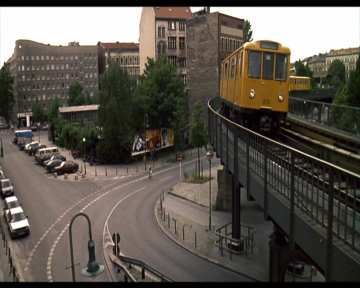
0     1     2     3     4     5     6     7     8     9
              0     -   219   223   134   195   266   187   275   206   287
              1   219     -   288   134   252   320   246   345   189   251
              2   223   288     -   178   215   232   208   341   190   231
              3   134   134   178     -   143   158   130   173   169   172
     (a)      4   195   252   215   143     -   228   210   259   174   270
              5   266   320   232   158   228     -   189   338   210   295
              6   187   246   208   130   210   189     -   278   171   199
              7   275   345   341   173   259   338   278     -   231   337
              8   206   189   190   169   174   210   171   231     -   204
              9   287   251   231   172   270   295   199   337   204     -

                    0     1     2     3     4     5     6     7     8     9
              0     -     2     3     6     4    13     1     6     2     3
              1     2     -     5     3     4    11    34     3     5     3
              2     3     5     -    14     2     6    10    10     8     4
              3     6     3    14     -     6     0     0     1    28     5
     (b)      4     4     4     2     6     -     1     7     0     3    23
              5    13    11     6     0     1     -     2     2     8     6
              6     1    34    10     0     7     2     -     2     4     3
              7     6     3    10     1     0     2     2     -     5    11
              8     2     5     8    28     3     8     4     5     -     1
              9     3     3     4     5    23     6     3    11     1     -

                    0     1    2      3    4     5     6     7     8      9
              0     -     0    1      1    0     8     0     0     0      0
              1     0     -    0      0    0     0    16     0     0      0
              2     1     0    -      1    0     0     0     5     1      1
              3     1     0    1      -    4     0     0     0    11      0
     (c)      4     0     0    0      4    -     0     0     0     2     14
              5     8     0    0      0    0     -     0     0     0      2
              6     0    16    0      0    0     0     -     0     0      0
              7     0     0    5      0    0     0     0     -     0      2
              8     0     0    1     11    2     0     0     0     -      0
              9     0     0    1      0   14     2     0     2     0      -

                    0     1     2     3     4     5     6     7     8     9
              0     -     0     0     0     0   163     0     0     0     0
              1     0     -     0     0     0     0   328     0     0     0
              2     0     0     -     0     0     0     0   137     0     0
              3     0     0     0     -     0     0     0     0    88     0
     (d)      4     0     0     0     0     -     0     0     0     9   290
              5   163     0     0     0     0     -     0     0     0     0
              6     0   328     0     0     0     0     -     0     0     0
              7     0     0   137     0     0     0     0     -     0     0
              8     0     0     0    88     9     0     0     0     -     0
              9     0     0     0     0   290     0     0     0     0     -

Table 1. Tables showing the number of matches found between the key frames of figure 5 at various

number of matches (darker indicates more matches). Frames and

stages of the matching algorithm. The image represents the table in each row with intensity coding the
                                                                          correspond. The diagonal entries
are not included. (a) matches from invariant indexing alone. (b) matches after neighbourhood consensus.
(c) matches after local correlation/registration verification. (d) matches after guided search and global
verification by robustly computing epipolar geometry. Note how the stripe corresponding to the correct
entries becomes progressively clearer.
Fig. 6. Verified feature matches after fitting epipolar geometry. It is hard to tell in these small images, but
each feature is indicated by an ellipse and lines indicate the image motion of the matched features between
frames. See figure 4 for a close-up of features. The spatial distribution of matched features also indicates
the extent to which the images overlap.

    Shots are represented here by key frames. The invariant descriptors are first computed in all
frames independently. The matching method then proceeds in four stages (described in more
detail below) with each stage using progressively stronger constraints: (1) Matching using the
invariant descriptors alone. This generates putative matches between the key frames but many
of these matches may be incorrect. (2) Matching using “neighbourhood consensus”. This is a
semi-local, and computationally cheap, method for pruning out false matches. (3) Local ver-
ification of putative matches using intensity registration and cross-correlation. (4) Semi-local
and global verification where additional matches are grown using a spatially guided search, and
those consistent with views of a rigid scene are selected by robustly fitting epipolar geometry.
    The method will be illustrated on 10 key frames from the movie ‘Run Lola Run’, one key
frame per shot, shown in figure 5. Statistics on the matching are given in table 1. ‘Run Lola Run’
is a time movie where there are three repeats of a basic sequence. Thus scenes typically appear
three times, at least once in each sequence, and shots from two sequences are used here.

Stage (1): Invariant indexing: By comparing the invariant vectors for each point over all
frames, potential matches may be hypothesized: i.e. a match is hypothesized if the invariant
vectors of two points are within a threshold distance. The basic query that the indexing structure
must support is “find all points within distance of this given point”. We take to be        times
the image dynamic range (recall this is an image intensity SSD threshold).
    For the experiments
                         in this paper we used a binary space partition tree, found to be more
time efficient than a -d tree, despite the extra overhead. The high dimensionality of the invariant
space (and it is generally the case that performance increases with dimension) rules out many
indexing structures, such as R-trees, whose performances do not scale well with dimension.
    In practice, the invariant indexing produces many false putative matches. The fundamental
problem is that using only local image appearance is not sufficiently discriminating and each
feature can potentially match many other features. There is no way to resolve these mismatches
using local reasoning alone. However, before resorting to the non-local stages below, two steps
are taken. First, as a result of using several (three in this case) sizes of elliptical region for
each feature it is possible to only choose the most discriminating match. Indexing tables are
constructed for each size separately (so for example the largest elliptical neighbourhood can
only match that corresponding size), and if a particular feature matches another at more than
one region size then only the most discriminating (i.e. larger) is retained. Second, some features
are very common and some are rare. This is illustrated in figure 7 which shows the frequency
of the number of hits that individual features find in the indexing structure. Features that are
common aren’t very useful for matching because of the combinatorial cost of exploring all the
possibilities, so we want to exclude such features from inclusion in the indexing structure. Our
method for identifying such features is to note that a feature is ambiguous for a particular
image if there are many similar-looking features in that image. Thus intra-image indexing is
first applied to each image separately, and features with five or more intra-image matches are
suppressed.

                   4.5                                                                       4.5                                                                   4.5                                                                4.5

                    4                                                                         4                                                                           4                                                                  4

                   3.5                                                                       3.5                                                                   3.5                                                                3.5

                    3                                                                         3                                                                           3                                                                  3

                                                                                                                                                       log10(frequency)

                                                                                                                                                                                                                          log10(frequency)
 log (frequency)

                                                                           log (frequency)

                   2.5                                                                       2.5                                                                   2.5                                                                2.5

                                                                                                                                                                          2                                                                  2
            10

                    2
                                                                                      10

                                                                                              2

                   1.5                                                                       1.5                                                                   1.5                                                                1.5

                    1                                                                         1                                                                           1                                                                  1

                   0.5                                                                       0.5                                                                   0.5                                                                0.5

                    0                                                                         0                                                                           0                                                                  0
                    −5   0   5   10    15       20     25   30   35   40                       0   5   10   15          20         25   30   35   40                          1   2   3   4       5       6   7   8   9                          1   2     3           4     5   6
                                      number of hits                                                             number of matches                                                        number of matches                                              number of matches

                                      (a)                                                                        (b)                                                                      (c)                                                            (d)

Fig. 7. The frequency of the number of hits for features in the invariant indexing structure for 10 key
frames. (a): Histogram for all features taken together. The highest frequency corresponds to features with
no matches, whilst some features have up to 30 matches. This illustrates that the density of invariant vectors


varies from point to point in invariant space. (b), (c), (d): Histograms for intra-image matching for each
of the three scales             . It is clear that features described at the smallest scale are strikingly less
distinctive than those described at higher scales. On the other hand, these have fewer matches as well.

Stage (2): Neighbourhood consensus: This stage measures the consistency of matches of

putative match between two images the         (
                                                     ) spatially closest features are determined in
spatially neighbouring features as a means of verifying or refuting a particular match. For each

each image. These      features define the neighbourhood set in each image. At this stage only
features which are matched to some other features are included in the set, but the particular fea-
                                                                ) neighbours have been matched, the
ture they are matched to is not yet used. The number of features which actually match between
the neighbourhood sets is then counted. If at least (
original putative match is retained, otherwise it is discarded.
    This scheme for suppressing putative matches that are not consistent with nearby matches
was originally used in [16, 21]. It is, of course, a heuristic but it is quite effective at removing
mismatches without discarding correct matches; this can be seen from table 1.

Stage (3): Local verification: Since two different patches may have similar invariant vectors, a
“hit” match does not mean that the image regions are affine related. For our purposes two points
are deemed matched if there exists an affine geometric and photometric transformation which
registers the intensities of the elliptical neighbourhood within some tolerance. However, it is too
expensive, and unnecessary, to search exhaustively over affine transformations in order to verify
every match. Instead an estimate of the local affine transformation between the neighbourhoods
is computed from the linear filter responses. If after this approximate registration the intensity
at corresponding points in the neighbourhood differ by more than a threshold, or if the implied
affine intensity change between the patches is outside a certain range, then the match can be
rejected.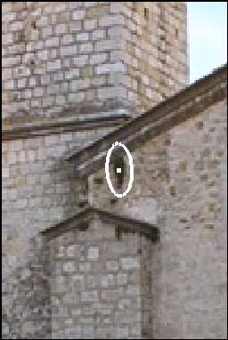
Stage (4): Semi-local and global verification: This stage has two steps: a spatially guided
search for new matches, and a robust verification of all matches using epipolar geometry. In
the first step new matches are grown using a locally verified match as a seed. The objective is
to obtain other verified matches in the neighbourhood, and then use these to grow still further
matches etc. Given a verified match between two views, the affine transformation between the
corresponding regions is now known and provides information about the local orientation of the
scene near the match. The local affine transformation can thus be used to guide the search for
further matches which have been missed as hits, perhaps due to feature localization errors, to be
recovered and is crucial in increasing the number of correspondences found to a sufficient level.
This idea of growing matches was introduced in [13]. Further details are given in [15].
    The second, and final, step is to fit epipolar geometry to all the locally verified matches
between the pair of frames. If the two frames are images of the same 3D scene then the matches
will be consistent with this two view relation (which is a consequence of scene rigidity). This is
a global relationship, valid across the whole image plane. It is computed here using the robust
RANSAC algorithm [18, 21]. Matches which are inliers to the computed epipolar geometry are
deemed to be globally verified.
Discussion: The number of matches for each of the four stages is given in table 1. Matching
on invariant vectors alone (table 1a), which would be equivalent to simply voting for the key
frame with the greatest number of similar features, is not sufficient. This is because, as dis-
cussed above, the invariant features alone are not sufficiently discriminating, and there are many
mismatches. The neighbourhood consensus (table 1b) gives a significant improvement, with the
stripe of correct matches now appearing. Local verification, (table 1c), removes most of the re-
maining mismatches, but the number of feature matches between the corresponding frames is
also reduced. Finally, growing matches and verifying on epipolar geometry, (table 1d), clearly
identifies the corresponding frames.
     The cost of the various stages is as follows: stage 1 takes
                                                                        seconds (intra+inter image
matching); stage 2 takes

                             seconds; stage 3 takes less than one millisecond; stage 4 takes
seconds (growing+epipolar geometry). In comparison feature detection takes a longer time by
far than all the matching stages.

Fig. 8. Matching results using three keyframes per shot. The images represent the normalized

matching matrix for the test shots under the four stages of the matching scheme.

    The matches between the key frames  and demonstrate well the invariance to change of
viewpoints. Standard small baseline algorithms fail on such image pairs. Strictly speaking, we
have not yet matched up corresponding frames because we have not made a formal decision,
e.g. by choosing a threshold on the number of matches required before we declare that two shots
match. In the example shown here, any threshold between 9 and 88 would do but in general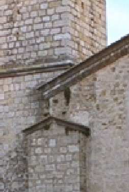
a threshold on match number is perhaps too simplistic for this type of task. As can be seen in
figure 6 the reason why so few matches are found for frames  and is that there is only a small
region of the images which do actually overlap. A more sensible threshold would also consider
this restriction.
Using several key frames per shot: One way to address the problem of small image overlap

is to aggregate the information present in each shot before trying to match. As an example, we
chose three frames (  frames apart) from each of the ten shots and ran the two-view matching
algorithm on the resulting set of
                                          frames. In the matrix containing number of
matches found, one would then expect to see a distinct
                                                            block structure. Firstly, along the
diagonal, the blocks represent the matches that can be found between nearby frames in each
shot. Secondly, off the diagonal, the blocks represent the matches that can be found between
frames from different shots. We coarsen the block matrix by summing the entries in each


block and arrive at a new and smaller    matrix
                                                            ; the diagonal entries now reflect how
easy it is to match within each shot and the off-diagonal entries how easy it is to match across


shots. Thus, the diagonal entries are used to normalize the other entries in the matrix by forming
a new matrix with entries given by                     (and zeroing its diagonal). Figure 8 shows
                                                                      block between matching
these normalized matrices as intensity images, for the various stages of matching.
     Note that although one would expect the entries within each
shots to be large, they can sometimes be zero if there is no spatial overlap (e.g. in a tracking
shot). However, so long as the three frames chosen for each shot cover most of the shot, there is
a strong chance that some pair of frames will be matched. Consequently, using more than one
key-frame per shot extends the range over which the wide baseline matching can be leveraged.

4 Conclusions and future work
We have shown in this preliminary study that wide baseline techniques can be used to match
shots based on descriptors which are ultimately linked to the shape of the 3D scene but mea-
sured from its image appearance. Using many local descriptors distributed across the image
enables matching despite partial occlusion, and without requiring prior segmentation (e.g. into
foreground/background layers).
    Clearly, this study must be extended to the 1000 or so shots of a complete movie, and a
comparison made with methods that are not directly based on 3D properties, such as colour
histograms and image region texture descriptions.


    In terms of improving the current method, there are two immediate issues: first, the com-

to
plexity is         in the number of key frames (or shots) used. This must be reduced to closer
          , and one way to achieve this is to use more discriminating (semi-)local descriptors
(e.g. configurations of other descriptors). Second, no use is yet made of the contiguity of frames
within a shot. Since frame-to-frame feature tracking is a mature technique there is a wealth of in-
formation that could be obtained from putting entire feature tracks (instead of isolated features)
into the indexing structure. For example, the measurement uncertainty, or the temporal stability,
of a feature can be estimated and these measures used to guide the expenditure of computational
effort; also, 3D structure can be used for indexing and verification. In this way the shot-with-
tracks will become the basic video matching unit, rather than the frames-with-features.

Acknowledgements

We are very grateful to Jiri Matas and Jan Palecek for supplying the MSE region code. Funding was
provided by Balliol College, Oxford, and EC project Vibes.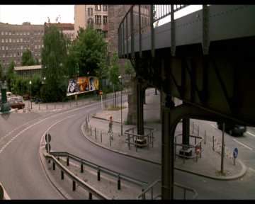
References
 1. A. Baumberg. Reliable feature matching across widely separated views. In Proc. CVPR, pages 774–
    781, 2000.
 2. M. Gelgon and P Bouthemy. Determining a structured spatio-temporal representation of video content
    for efficient visualization and indexing. In Proc. ECCV, pages 595–609, 1998.
 3. R. I. Hartley and A. Zisserman. Multiple View Geometry in Computer Vision. Cambridge University
    Press, ISBN: 0521623049, 2000.
 4. H. Lee, A. Smeaton, N. Murphy, N. O’Conner, and S. Marlow. User interface design for keyframe-
    based browsing of digital video. In Workshop on Image Analysis for Multimedia Interactive Services.
    Tampere, Finland, 16-17 May, 2001.
 5. R. Lienhart. Reliable transition detection in videos: A survey and practitioner’s guide. International
    Journal of Image and Graphics, Aug 2001.
 6. T. Lindeberg and J. Gårding. Shape-adapted smoothing in estimation of 3-d depth cues from affine
    distortions of local 2-d brightness structure. In Proc. ECCV, LNCS 800, pages 389–400, May 1994.
 7. J. Matas, J. Burianek, and J. Kittler. Object recognition using the invariant pixel-set signature. In Proc.
    BMVC., pages 606–615, 2000.
 8. J. Matas, O. Chum, M. Urban, and T. Pajdla. Distinguished regions for wide-baseline stereo. Research
    Report CTU–CMP–2001–33, Center for Machine Perception, K333 FEE Czech Technical University,
    Prague, Czech Republic, November 2001.
 9. J Matas, M Urban, and T Pajdla. Unifying view for wide-baseline stereo. In B Likar, editor, Proc.
    Computer Vision Winter Workshop, pages 214–222, Ljubljana, Sloveni, February 2001. Slovenian
    Pattern Recorgnition Society.
10. K. Mikolajczyk and C. Schmid. Indexing based on scale invariant interest points. In Proc. ICCV,
    2001.
11. K. Mikolajczyk and C. Schmid. An affine invariant interest point detector. In Proc. ECCV. Springer-
    Verlag, 2002.
12. P. Pritchett and A. Zisserman. Matching and reconstruction from widely separated views. In R. Koch
    and L. Van Gool, editors, 3D Structure from Multiple Images of Large-Scale Environments, LNCS
    1506, pages 78–92. Springer-Verlag, Jun 1998.
13. P. Pritchett and A. Zisserman. Wide baseline stereo matching. In Proc. ICCV, pages 754–760, Jan
    1998.
14. F. Schaffalitzky and A. Zisserman. Viewpoint invariant texture matching and wide baseline stereo. In
    Proc. ICCV, Jul 2001.
15. F. Schaffalitzky and A. Zisserman. Multi-view matching for unordered image sets, or “How do I
    organize my holiday snaps?” . In Proc. ECCV. Springer-Verlag, 2002. To appear.
16. C. Schmid and R. Mohr. Local greyvalue invariants for image retrieval. IEEE PAMI, 19(5):530–534,
    May 1997.
17. D. Tell and S. Carlsson. Wide baseline point matching using affine invariants computed from intensity
    profiles. In Proc. ECCV, LNCS 1842-1843, pages 814–828. Springer-Verlag, Jun 2000.
18. P. H. S. Torr and D. W. Murray. The development and comparison of robust methods for estimating
    the fundamental matrix. IJCV, 24(3):271–300, 1997.
19. T. Tuytelaars and L. Van Gool. Content-based image retrieval based on local affinely invariant regions.
    In Int. Conf. on Visual Information Systems, pages 493–500, 1999.
20. T. Tuytelaars and L. Van Gool. Wide baseline stereo matching based on local, affinely invariant
    regions. In Proc. BMVC., pages 412–425, 2000.
21. Z. Zhang, R. Deriche, O. D. Faugeras, and Q.-T. Luong. A robust technique for matching two un-
    calibrated images through the recovery of the unknown epipolar geometry. Artificial Intelligence,
    78:87–119, 1995.
You can also read