An Image-based Approach of Task-driven Driving Scene Categorization
←
→
Page content transcription
If your browser does not render page correctly, please read the page content below
An Image-based Approach of Task-driven Driving Scene Categorization
                                                      Shaochi Hu1 , Hanwei Fan1 , Biao Gao1 , Xijun Zhao2 and Huijing Zhao1 , Member, IEEE

                                            Abstract— Categorizing driving scenes via visual perception
                                         is a key technology for safe driving and the downstream
                                         tasks of autonomous vehicles. Traditional methods infer scene
                                         category by detecting scene-related objects or using a classifier
                                         that is trained on large datasets of fine-labeled scene images.
                                         Whereas at cluttered dynamic scenes such as campus or park,
arXiv:2103.05920v1 [cs.RO] 10 Mar 2021

                                         human activities are not strongly confined by rules, and the
                                         functional attributes of places are not strongly correlated with
                                         objects. So how to define, model and infer scene categories
                                         is crucial to make the technique really helpful in assisting
                                         a robot to pass through the scene. This paper proposes a
                                         method of task-driven driving scene categorization using weakly
                                         supervised data. Given a front-view video of a driving scene,
                                         a set of anchor points is marked by following the decision
                                         making of a human driver, where an anchor point is not a
                                         semantic label but an indicator meaning the semantic attribute                 Fig. 1: The difficulty of categories definition in cluttered
                                         of the scene is different from that of the previous one. A
                                         measure is learned to discriminate the scenes of different                     dynamic scenes.
                                         semantic attributes via contrastive learning, and a driving
                                         scene profiling and categorization method is developed based                   into a scene label, and supervised learning [7] are conducted
                                         on that measure. Experiments are conducted on a front-view                     mostly which require a large amount of fine-labeled datasets.
                                         video that is recorded when a vehicle passed through the
                                                                                                                           MIT place [8] and Large Scene understanding (LSUN)
                                         cluttered dynamic campus of Peking University. The scenes are
                                         categorized into straight road, turn road and alerting traffic.                [9] datasets contain a large number of labeled images that
                                         The results of semantic scene similarity learning and driving                  were originally downloaded from websites by using Google
                                         scene categorization are extensively studied, and positive result              and other image search engines. Honda [7] and FM3 [10]
                                         of scene categorization is 97.17 % on the learning video and                   datasets are more motivated by robotic and autonomous
                                         85.44% on the video of new scenes.
                                                                                                                        driving applications, which contain egocentric videos of
                                                                                                                        driving scenes that are labeled at the frame level. Scene
                                                                I. INTRODUCTION                                         labels (i.e. categories) of these datasets are mainly defined on
                                            Human activities are strongly connected with the semantic                   the following aspects: (1) functional attribute of places, e.g.
                                         attributes of scene objects and regions. For example, the                      cafeteria, train station platform [8], intersection, construction
                                         zebra-zone defines a region where pedestrians cross the road;                  zone [7]; (2) a target object of the scene, e.g. people, bus
                                         traffic signal prompts an intersection where a mixture of                      [9], overhead bridge [10]; (3) the static status of the target
                                         traffic flows happen, etc. Categorizing driving scene via                      object or scene, e.g. road surface, weather condition [7]; (4)
                                         environmental perception is a key technology for safe driving                  the dynamic status of the agent with respect to the scene,
                                         and the downstream tasks of autonomous vehicles such as                        e.g. approaching, entering and leaving an intersection [7].
                                         object detection, behavior prediction and risk analysis, etc.                     However, scene categorization based on the above cate-
                                            Place/scene categorization [1] or scene classification [2]                  gory definitions may be less helpful for a robot to traverse
                                         belongs to the same group of researches, which has been                        cluttered dynamic urban scenes. For scenes shown in Fig. 1,
                                         studied broadly in the robotic field such as semantic mapping                  the functional attributes of places are not clearly defined, e.g.
                                         [3] or navigating a robot using scene-level knowledge [4].                     pedestrians can walk on sidewalk or motorway, intersections
                                         Many methods infer scene category by detecting certain                         have neither traffic signal nor zebra-zone, and pedestrians
                                         objects that have unique functions in specific scenes, such as                 cross the road anywhere. On the other hand, categorizing
                                         bed for a bedroom or knife for a kitchen [5] [6]. Deep learn-                  scenes on the presence of certain objects is less meaningful
                                         ing methods have been the vast majority of the researches in                   as the scenes are populated, complex and are usually not
                                         recent years, where a CNN is trained to map the input image                    associated with any special objects. For example, pedestrians,
                                                                                                                        cyclists or cars may appear anywhere, whereas the agent
                                            This work is supported in part by the National Natural Science Foundation   needs to make a special handle only when potential risks
                                         of China under Grant 61973004                                                  are detected. How to define semantically meaningful scene
                                            1 S.Hu, H.Fan, B.Gao and H.Zhao are with the Key Lab of Machine
                                                                                                                        categories is crucial to make the scene categorization results
                                         Perception (MOE), Peking University, Beijing, China. 2 X.Zhao is with
                                         China North Vehicle Research Institute, Beijing, China                         really helpful in the tasks such as assisting human drivers or
                                            Correspondence: H. Zhao, zhaohj@cis.pku.edu.cn.                             autonomous driving at cluttered dynamic urban scenes.
This research proposes a task-driven driving scene catego-     3&4&4-way intersection, overhead bridge, rail crossing,
rization method by learning from the human driver’s decision      tunnel, zebra crossing, where FM3 defines 8 traffic scene:
making. The normal state of an experienced human driver           highway, road, tunnel, exit, settlement, overpass, booth,
is usually relaxed. He/she is alerted when the situation is       traffic. They are both collected by an on-board RGB camera
different from normal, such as a potential danger, or when        and annotated by human operators. Their label definition
the situation changes from the early moment (i.e. scenes          focuses on the road static structure regardless of the dynamic
with different semantic attributes), such as approaching an       of traffic.
intersection. Given a video of driving scene, we let a               MIT place [8] and Large Scene understanding (LSUN) [9]
human driver mark the scenes with sparse anchor points,           datasets contain a large number of labeled images that were
where a pair of successive anchor points denote scenes of         originally downloaded from websites by using Google and
different semantic attributes. Inspired by the recent progress    other image search engines, and then annotated by human.
on contrastive learning [11] and the impressive results in        MIT place dataset has up to 476 fine-grained scene categories
visual feature representation [12] and metrics learning [13],     including from indoor to outdoor such as romantic bedroom,
our research learns a semantic scene similarity measure via       teenage bedroom, bridge and forest path, etc. LSUN has only
anchor points using contrastive learning, which is exploited      10 scene categories: bedroom, kitchen, living room, dining
to profile scenes of different categories, and further infer      room, restaurant, conference room, bridge, tower, church,
scene labels for both online and offline applications such        outdoor. They are labeled mainly by the functional attribute
as semantic mapping and driving assistant. Experiments are        of a place and the target object of the scene.
conducted using a front-view video that was collected when           The above categories definition may be less helpful for
a vehicle drived through a cluttered dynamic campus. The          our task-driven driving scene categorization problem which
scenes are categorized into straight road (normal driving         focuses on cluttered dynamic urban scenes.
with no alerting traffic), turn road and alerting traffic. The
proposed method is extensively examined by experiments.           C. Contrastive Learning
                                                                     Self-supervised learning [20] aims at exploring the internal
                   II. R ELATED W ORKS                            distribution of data by constructing a series of tasks using
A. Scene Categorization Method                                    different prior knowledge of images. Recent progress in
   Many methods infer scene category by detecting certain         self-supervised learning mainly contributed by contrastive
objects that have unique functions in specific scenes. [6]        learning [11], which effectively represents image feature by
combines object observations, the shape, size, and appear-        training InfoNCE loss [21] on delicately constructed positive
ance of rooms into a chain-graph to represent the semantic        and negative samples. Memory-based method [22] [23] suffer
information and perform inference. [14] learns object-place       from the old feature in memory resulting in less consistent
relations from an online annotated database and trains object     for the update of the network, and the performance of end-
detectors on some of the most frequently occurring objects        to-end approach [24]–[26] are limited by the GPU memory.
by hand-crafted features. [15] uses common objects, such as       Moco [27] makes a balance between feature updating and
doors or furniture, as a key intermediate representation to       memory size by maintaining a queue and momentum updat-
recognize indoor scenes.                                          ing the network. SimCLR [28] improves the performance by
   Motivated by the success of deep learning in addressing        applying a projection head at the end of the network.
visual image recognition tasks, CNN has been widely used                              III. M ETHODOLOGY
as a feature encoder or mapping function of image and label
for scene categorization in robotics. [16] presents a part-       A. Problem Formulation
based model and learns category-specific discriminative parts        A front-view video V of a driving scene is marked by a hu-
for the part-based model. [17] represents images as a set of      man driver with a set of anchor points K = {k1 , k2 , ..., kn },
regions by exploiting local deep representations for indoor       where ki is a frame index of the video, and an anchor
image place categorization. [18] trains a discriminative deep     point ki means that the semantic attribute A of the driving
belief network (DDBN) classifier on the GIST features of the      scene captured by image frame V (ki ) is different from that
image. Driving scene categorization is conducted in [19] by       of the previous anchor point ki−1 , i.e. A(ki ) 6= A(ki−1 ).
combining the features representational capabilities of CNN       Without loss of generality, we assume that the driving scenes
with the VLAD encoding scheme, and [7] trains an end-to-          captured by video V is temporally continuous, i.e. A(ki ) =
end CNN for this task.                                            A(ki + δ) and A(ki ) 6= A(ki−1 + δ), where δ is a small
                                                                  integer indicating the neighbor frames of an anchor point
B. Scene Category Definition                                      (neighborhood consistent assumption).
  Here we review some typical scene categorization datasets,         Given a video V and a set of anchor points K for training,
and we focus on their label definition, data acquisition and      this work is to learn a scene profiler to model the driving
annotation method.                                                scenes of different semantic categories C such as straight
  Honda [7] and FM3 [10] datasets focus on driving scene          road and turn road, and further infer scene labels for both
categorization, and Honda defines 12 typical traffic scenarios:   online and offline applications such as semantic mapping and
branch left, branch right, construction zone, merge left,         driving assistant.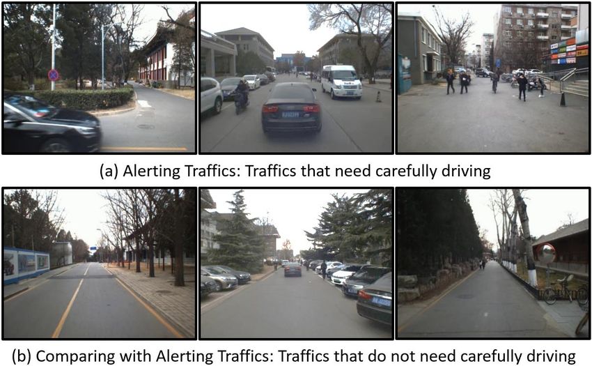
Fig. 2: Algorithm pipeline. The training detail of fθ is shown in Sec. III-C, and the above fθ share weights. The
implementation of DS and ScP are shown in Sec. III-D.1 and III-D.2.

   To make the scene labels semantically meaningful, the            However, the scenes of a complex driving environment
categories of semantic scenes C are predefine by a human         are not clearly separable in feature space ZD as shown in
operator, which is represented by a typical image frame qc       Fig. 5(b), and the clusters of z might not be semantically
for each scene category c.                                       meaningful. This research proposes a method to use the
   This research studies method of using a single image as       distribution of semantic scene similarity (DS) as a signature
input, which could be extended in the future by inferring on     for scene profiling and labeling. Given a manually selected
video clips.                                                     image frame qc which presents the typical scene of category
B. Outline of the Method                                         c, an average DS is estimated as a meta pattern of the scene
                                                                 category (scene category profile, ScP). During inference,
   The method is composed of two modules: 1) semantic
                                                                 given an image frame, its DS is first estimated, and then
scene similarity learning, 2) driving scene profiling and
                                                                 is compared with the ScP of each category. The scene label
labeling. The workflow is shown in Fig. 2.
                                                                 is predicted as the best-match one on the semantic scene
   Semantic scene similarity learning is to find a measure to
                                                                 similarity distribution. The implementation details are shown
evaluate the semantic similarity of any two scenes, which
                                                                 in Sec. III-D.
is supervised by the anchor points and the neighborhood
consistent assumption for semantically different and similar
                                                                 C. Semantic Scene Similarity Learning
scenes. Let zi = fθ (i) be a feature encoder converting a
high-dimensional image i to a low-dimensional normalized            1) Sampling Strategy: For a given query point q ∈
feature vector z ∈ ZD . The semantic scene similarity of         [ki , ki + δ] of video V , where ki is an anchor point and δ is
a pair of image (i, j) is measured in feature space ZD on        a small integer as mentioned at the beginning of Sec. III-A,
cosine similarity sim(i, j) = ziT · zj . In feature space ZD ,   its one positive sample and n negative samples are selected
zi and zj are pushed away from each other if they are of two     by the neighborhood consistent assumption for contrastive
successive anchor points respectively, whereas pulled close if   learning training.
they are in the neighborhood of a same anchor point, and this       The positive sample q + is randomly selected near the
pull-push process is implemented by contrastive learning.        anchor point ki , that is q + ∈ [ki , ki + δ] . The n negative
The implementation details are shown in Sec. III-C.              samples {qj− |j = 1, ..., n} are randomly selected near the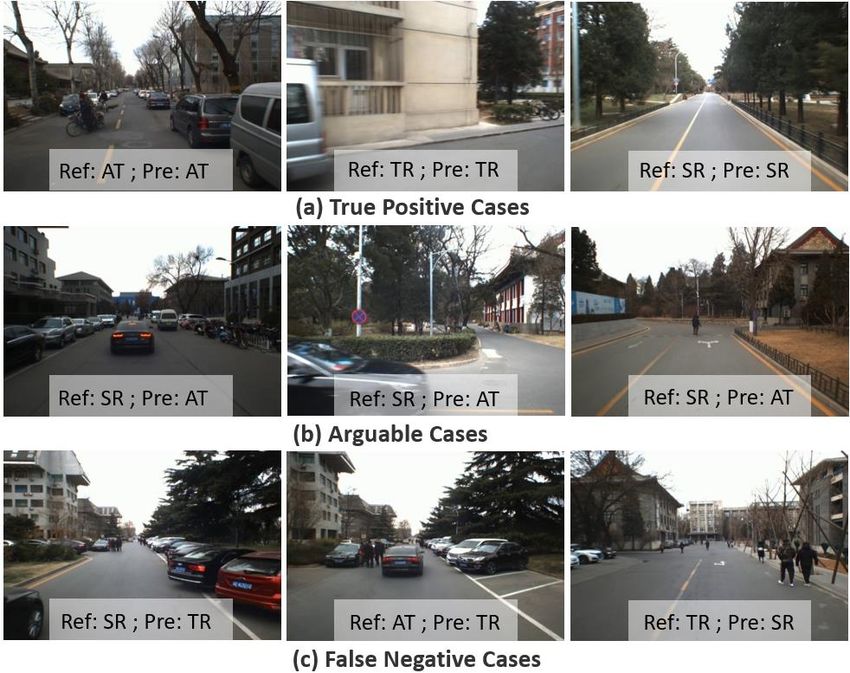
Fig. 3: Case study of Distribution of Semantic Scene Similarity (DS) and Scene Category Profile (ScP).
two successive anchor points of ki , that is qj− ∈ [ki−1 , ki−1 +   the distributions are in fact related with road geometry and
δ] ∪ [ki+1 , ki+1 + δ], as shown in Fig. 2.                         dynamic traffic of the scene, which is further investigated
   2) Network Design and Loss Function: Feature encoder             through experiments in Sec. IV-C.1.
fθ is implemented by AlexNet [29] to convert 3-channel                 Therefore, a method of driving scene profiling and labeling
RGB image into 128-dimension feature vector z ∈ ZD=128 ,            is designed on DS, which is composed of learning semantic
and it is trained by contrastive learning method with In-           scene category profiles, and inferring scene labels for both
foNCE loss [21]:                                                    online and offline applications.
                           exp(zqT · zq+ /τ )                          2) Scene Category Profile (ScP): A set of DS is estimated
  L = −log                       Pn                          (1)    D = {ds(p)|p ∈ V } on each image frame p of the training
             exp(zqT · zq+ /τ ) + j=1 exp(zqT · zq− /τ )            video V . For a semantic scene category c, given a typical
                                                     j

   3) Learning Result: As mentioned in Sec. III-B, the              image frame qc of it by human operator, the DS of qc ,
semantic scene similarity of a pair of image (i, j) is measured     denoted as ds(qc ), is compared with all the ds(p) in D by
in feature space ZD by cosine similarity sim(i, j) = ziT · zj .     Jensen-Shannon Divergence JS-D(ds(qc ), ds(p)) to evaluate
                                                                    the divergence of semantic similarity distributions. The ds(p)
D. Driving Scene Categorization                                     is gathered if JS-D(ds(qc ), ds(p)) < σ, and an average
   1) Distribution of Semantic Scene Similarity (DS): Given         distribution of the gathered ds(p) are taken as the scene
a query image q, semantic scene similarity is measured              category profile of category c, which is denoted as scp(c).
between q and each image frame p of the training video              Here σ is a pre-define threshold. A pseudo-code is given in
V , and a set of similarity values are obtained Ω(q) =              Algorithm1
{sim(q, p)|p ∈ V }. A histogram is subsequently generated              Here is a question: How the selection of the typical image
on Ω(q) to find the distribution of semantic scene similarity       frame qc of the category c influence scp(c)? As shown in
(DS), which is used as a descriptor of the scene q denoted          Fig. 3(b), for each category, several typical scene frames qc
as ds(q). Such a descriptor captures semantically meaningful        of it are selected to estimate its ScP respectively. It can be
pattern as examined in Fig. 2.                                      found that even the typical scene frames qc of a category
   As shown in Fig. 3(a), by randomly choosing semanti-             are selected at very different locations, the generated ScP
cally typical scenes on straight road, turn road and alerting       are very similar. It demonstrates that the method is robust to
traffic respectively in different regions, samples of DS are        typical scene frame selection and able to capture the meta
estimated, and it can be found that the DS of the same              pattern of the scene category.
scene category show similar pattern. The peaks and valleys of          3) Scene Category Reasoning: In reasoning, given the
                                                                    current image frame q, ds(q) is estimated by measuring
                                                                    semantic similarity between q and the image frames of the
 Algorithm 1: Calculating ScP of category c                         training video V and finding the distribution. Comparing
  Input: D = {ds(p)|p ∈ V }, meaning DS of all                      ds(q) with each scp(c) of category c ∈ C by Jensen-Shannon
          training video frames                                     Divergence JS-D(ds(q), scp(c)), the c of the minimal diver-
  Input: A manually selected typical image qc of                    gence, i.e. the most matched distribution, is found as the
          category c                                                predicted label cq of the current scene q, i.e.
  Output: ScP of category c, denoted as scp(c)                                   cq = argmin JS-D(ds(q), scp(c))               (2)
1 DSList = [];                                                                           c∈C
2 for p ∈ V do                                                                     IV. E XPERIMENTAL R ESULTS
3     if JS-D(ds(qc ), ds(p)) < σ then
                                                                    A. Experimental Data and Design
4         DSList.append(ds(p))
5     end                                                              1) Video Data: An egocentric video is collected in the
6 end                                                               campus of Peking University by using a front-view monoc-
7 scp(c) = Average(DSList)                                          ular RGB camera. Fig. 4(a) shows the driving route that
                                                                    covers a broad and diverse area containing teaching and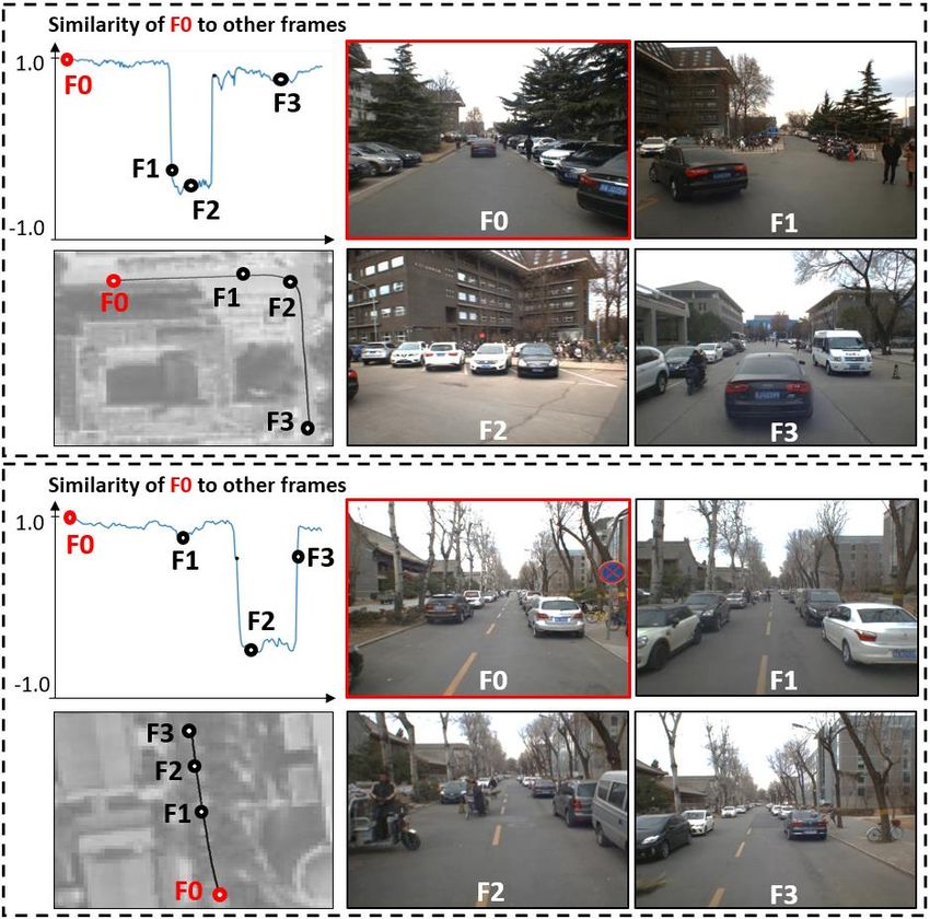
Fig. 4: Experimental data illustration.
research zone (A), residential zone (B) and landscape zone         developing reference labels via anchor points to assist in
(C). Fig. 1 shows typical road scenes, where pedestrians,          analyzing the experimental results. Since the anchor points
cyclists and cars are populated, and the behaviors of road         are marked whenever a human driver notice a change of
users are not strongly confined by traffic rules. A 20-minute      scene attribute, although there might be some delay due to
video is recorded with 36924 image frames at a frame rate          the response time of conscious, the anchor points could serve
of 30 fps, where the teaching and research zone (A) are            as inaccurate delimiters to divide the stream of image frames
recorded twice but at different time as it is the start and end    into semantically different segments, and each segment is
position of the driving route. In order to discriminate, we        assigned a single label by the human driver while marking
call the second drive at the teaching and research zone as         the anchor points. As shown in Fig. 4(c), the reference labels
(D).                                                               of SR, TR and AT are developed on the image frames of both
   2) Anchor Point: The video is divided into two parts in         parts videos.
experiments as shown in Fig. 4(a). Part I covers zone A-              4) Experiment Design: Experiments are conducted on two
B-C that is marked by a human driver with anchor points,           levels: (1) Semantic Scene Similarity Learning (Sec. IV-B).
while part II covers zone D that is unmarked, representing         Two experiments are conducted to examine the performance
scenes of the same location with zone A but has different          of semantic scene similarity learning, where the scenes
routes and dynamic traffics. A total of 242 anchor points are      are categorized with two and three labels respectively. The
marked on the video frames by a human driver to imitate            results are analyzed at the levels of feature vector, trajectory
his decision making during driving. A new anchor point is          point and image frame. (2) Driving Scene Categorization
marked when the driver recognize a change of the scene             (Sec. IV-C). The results of semantic scene profiling based on
attribute, which may cause a different handling in driving or      the distribution of similarity evaluation are first explanatory
a mental state change. Fig. 4(b) shows an example, where the       analyzed, and two experiments on scene categorization are
first anchor point (red) is marked at the frame k1 of a straight   then conducted, which aim at demonstrating the performance
road scene, the second is at the frame k2 when the vehicle         towards the offline and online applications such as semantic
enters a turn, and the third is at the frame k3 after the turn     mapping and scene label prediction.
finished. Similarly, anchor points are marked when the driver      B. Semantic Scene Similarity Learning
is alerted by other road users in the scene. A neighbor frame         1) Metrics Learning: In order to examine the performance
(black) of k1 and k2 is also shown and denoted as k1 + δ           of semantic scene similarity learning, a two-category ex-
and k2 + δ respectively, which demonstrates the consistence        periment is specially conducted, in addition to the three-
of semantic scene attribute in neighborhood.                       category one as designed in the previous subsection. In this
   3) Scene Category and Reference Label: In this experi-          experiment, the two scene categories are straight road (ST)
ment, scenes are categorized with three semantic labels, i.e.      and turn road (TR). The anchor points alerting traffic (AT)
SR: straight road, TR: turn road, AT: alerting traffic. Both       are removed from the original set, and the reference labels
SR and AT happen on straight roads, which are differentiated       AT of the video segments are changed to ST. The results of
on whether there are other road users who need to be alert         both two- and three-category learning are shown in Fig. 5.
in the scene. As the period of the vehicle turning is short,          Given the video part I and the set of marked anchor points,
and drivers are usually very concentrated, TR is not further       each experiment learns a feature representation fθ following
divided into alerting or non-alerting traffics.                    the method described in Sec. III-C, where for each query
   Manually assigning semantic labels to each image frame is       point q, one positive and n = 16 negative samples are
nontrivial, because the operator will always ask the question:     randomly taken to estimate the InfoNCE loss of Eqn.1. With
when are the start and the end image frames of the same            the learned fθ , each image is converted into a feature vector
semantic attribute? Whereas the answer is not clearly defined.     z ∈ ZD , where D = 128 in this research. For visualization,
So in this research, we do not have Ground Truth, but              these feature vectors are further reduced to 2 dimension using
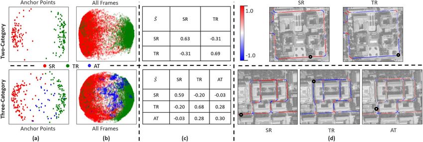
Fig. 5: Illustration of semantic scene similarity at the level of feature and trajectory. (a)&(b) Visualization of feature after
dimension reduction. (c) Similarity of scene categories. (d) Similarity between the query frame (black point) and trajectory.
PCA, and colored on their reference labels and shown in shown respectively, where F0 is the query frame q of normal
Fig. 5(a)&(b). In Fig. 5(a), it can be found that the anchor straight road scenes (SR). The similarity values of the sub-
points are clustered in different zones that are consistent sequent frames with F0 are plotted, which show a dramatic
with their reference labels (i.e. semantic meaning) in both down-and-up pattern, and we can find that the image frames
two- and three-category results. Whereas when testing all of lower similarity values are scenes of semantically different
image frames, as visualized in Fig. 5(b), the feature vectors attributes with F0, e.g. F1-F2 are turn road in the top case
of different colors can not be easily separated. and F2 is alerting traffic in the bottom case.
2) Performance Analysis: To further analyze the results, The above results show that the proposed method has
a new metric is defined as below to evaluate similarity of efficiency in learning a semantically meaningful metric to
two scene categories: evaluate the similarity/distance of dynamic driving scenes.
X 1
S̃(c1 , c2 ) = · sim(p, q)
p∈c ,q∈c
|c1 | · |c2 |
1 2
where S̃(c1 , c2 ) ∈ [−1, 1], |c1 | and |c2 | denote the image
number of category c1 and c1 respectively, and sim(p, q)
is the semantic scene similarity of two images on cosine
similarity of their feature vectors zp and zq as mentioned
before. The lower the S̃, the more separable of the two
categories and the better performance of the learned fθ . As
shown in Fig. 5(c), comparing to the diagonal values repre-
senting intra-category similarities, the off-diagonal ones of
inter-category similarities are much lower, meaning that the
learning method has efficiency from a statistical viewpoint.
On the other hand, as shown in Fig. 5(d), randomly select
a query frame q (black point) with reference label of SR,
TR or AT, find its similarity with all other image frames of
the video, i.e. ∀p ∈ V, sim(p, q), and visualize the similarity
values by coloring the trajectory points. Red for similar (1.0),
blue for dissimilar (-1.0). The colors change with the selected
query frame q. Given a query frame of reference label SR,
it can be found that all trajectory points on turn roads are
blue, and the straight roads are mainly red. Given a query Fig. 6: Illustration of semantic scene similarity at the level
frame of reference label TR, the trajectory points are mainly of image frame.
red on turn roads whereas blue on straight roads. Given a
query frame of reference label AT, most trajectory points are
colored from blue to light red. C. Driving Scene Categorization
Fig. 6 further illustrates the similarity values at the level of 1) Semantic Scene Profiling: Based on the distribution
image frames. Two cases of traversing through a turn road of semantic scene similarity (DS), profiles are generated for
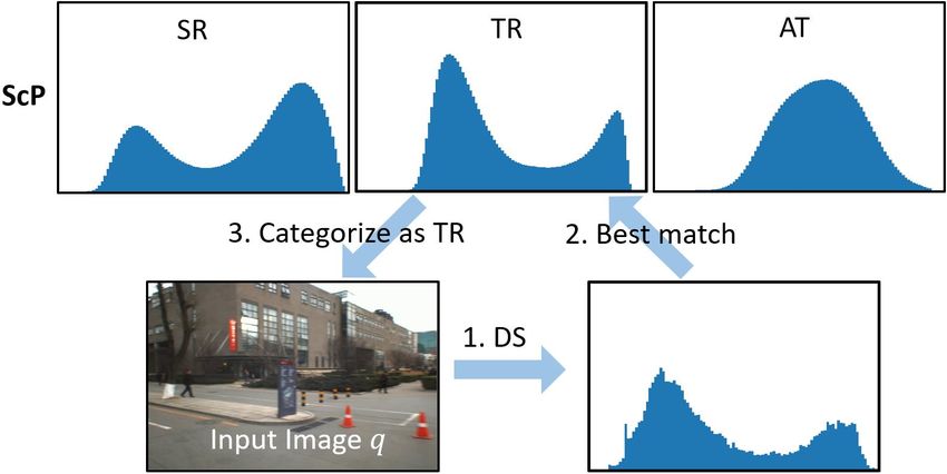
(top of Fig. 6) and alerting traffic (bottom of Fig. 6) are scene categories (ScP) of SR, TR and AT via typical image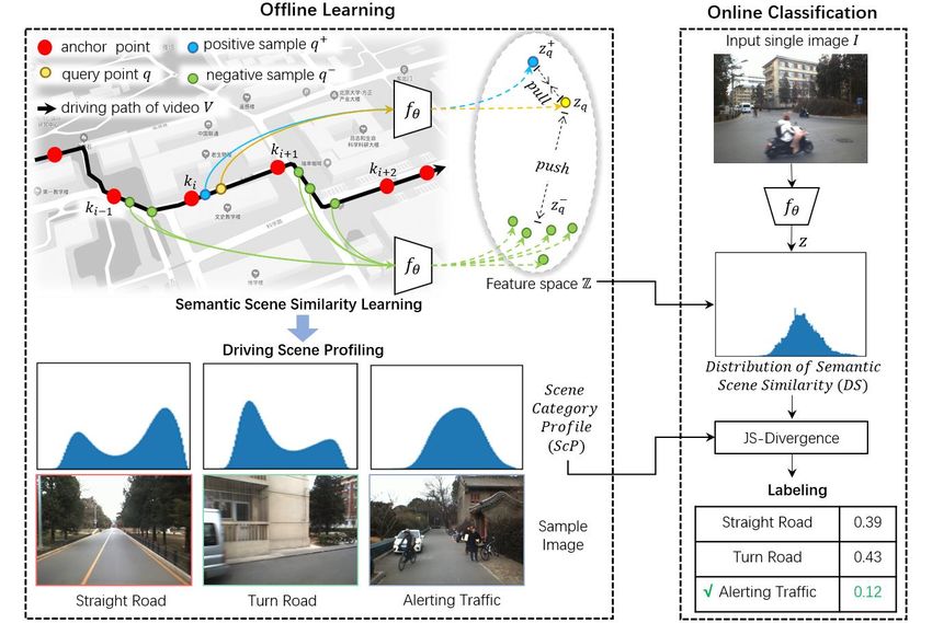
q of an offline video or from an online camera, its DS is first
estimated by evaluating semantic similarity with the image
frames of the training video, and then compared with the
scene category profiles (ScP) to find the category c of the
best match scp(c). For a given 224 × 224 × 3 RGB image,
it take 50 ms to get its feature on NVIDIA GTX 1080, and
0.8 ms to calculate its DS, and 0.2 ms to find the best match
ScP of all categories on Intel Core i9 using Python.
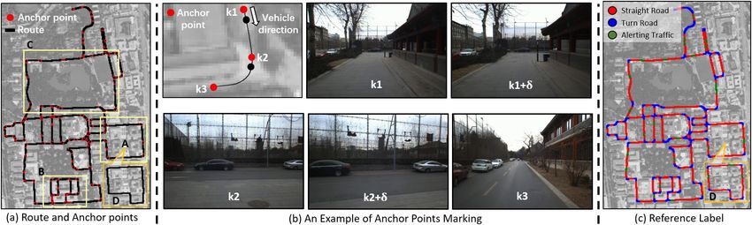
Scene categorization results on both video part I and II are
shown in Fig. 9(a). By comparing with the reference labels,
Fig. 7: Explanatory analysis of semantic scene profiling the results are divided into three types as shown in Fig. 9(b).
based on the distribution of similarity. True Positive (TP) are those matched with the reference
labels. The rest set of unmatched results is examined by
frames as shown in Fig. 3. The peaks and valleys of the DS a human driver, where two different types are discovered:
and ScP are related with the road geometry and dynamic False Negative (FN) are those of wrong categorizations,
traffic of the scenes. Fig. 7 examines the components of while Arguable (AG) are arguable results. Fig. 10 shows
the DS of each category, where the DS is estimated by first examples of True Positive (TP), False Negative (FN) and
selecting a typical scene q, and then estimating the semantic Arguable(AG) results where Ref is the reference label and
scene similarity Ω(q) = {sim(q, p)|p ∈ V }, and finally Pre is the predicted label.
generating a histogram on Ω(q). The similarity values can be Since reference labels are generated on the set of anchor
divided into three types according to their reference labels, points marked when watching the video, the human decision
therefore colored bar charts can be generated to visualize the is made on image sequences, so even a driver just encounters
contributions of each component. a situation like Fig. 10(b), the scenes will not be marked as
Take straight road scenes as example shown in Fig. 7(a), alerting traffic, as the decision is made based on the predic-
the right (high similarity) and left (low similarity) peaks of tion of other road users’ tendency. However, this research
DS are respectively contributed from straight and turn road develops a single-image-based algorithm. Therefore, such
scenes, and the area of the peaks reflects the proportion results are counted as Arguable (AG) as they are reasonable
of straight and turn roads in the scene frames, e.g. in an results with the input of single images.
environment dominated by straight roads, the right peak
could be very sharp and tall, whereas in an environment TABLE I: Three types of categorization results.
of various road types, the right peak could be wide and flat. Anchor points TP AG FN
Turn road scenes are the opposite shown in Fig. 7(b). The DS Video part I 3 74.82% 22.35% 2.83%
of alerting traffic is different from straight and turn roads as Video part II 5 56.64% 28.80% 14.56%
shown in Fig. 7(c), which is a single-peak pattern. Comparing
to straight and turn road scenes, alerting traffic is a minority, These three types of results are counted in TABLE I.
whereas the density and distribution could be a significant The video part I is marked with anchor points for learning,
feature to describe the dynamic traffic of the scene. and this experiment demonstrates the performance for offline
2) Scene Categorization: Experiments are conducted on
video part I with marked anchor points for learning and
video part II of new scenes, aiming at performance validation
towards offline applications such as semantic mapping and
online applications such as scene label prediction. Both
experiments are conducted in the same procedure that is
demonstrated in Fig. 8 by case result. Given an image frame
Fig. 9: Scene categorization results. (a) The predicted label.
Fig. 8: Categorization procedure. (b) Comparing with reference label.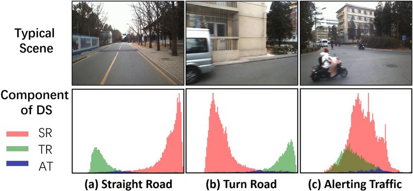
R EFERENCES
                                                                  [1] N. Sünderhauf et al., “Place categorization and semantic mapping on
                                                                      a mobile robot,” in ICRA. IEEE, 2016, pp. 5729–5736.
                                                                  [2] J. C. Rangel et al., “Scene classification based on semantic labeling,”
                                                                      Advanced Robotics, vol. 30, no. 11-12, pp. 758–769, 2016.
                                                                  [3] I. Kostavelis et al., “Semantic mapping for mobile robotics tasks: A
                                                                      survey,” Robotics and Autonomous Systems, vol. 66, pp. 86–103, 2015.
                                                                  [4] I. Kostavelis, “Robot navigation via spatial and temporal coherent
                                                                      semantic maps,” Engineering Applications of Artificial Intelligence,
                                                                      vol. 48, pp. 173–187, 2016.
                                                                  [5] Y. Liao et al., “Understand scene categories by objects: A semantic
                                                                      regularized scene classifier using convolutional neural networks,” in
                                                                      ICRA. IEEE, 2016, pp. 2318–2325.
                                                                  [6] A. Pronobis et al., “Large-scale semantic mapping and reasoning with
                                                                      heterogeneous modalities,” in ICRA. IEEE, 2012, pp. 3515–3522.
                                                                  [7] A. Narayanan et al., “Dynamic traffic scene classification with space-
                                                                      time coherence,” in ICRA. IEEE, 2019, pp. 5629–5635.
                                                                  [8] B. Zhou et al., “Learning deep features for scene recognition using
                                                                      places database,” 2014.
                                                                  [9] F. Yu et al., “Lsun: Construction of a large-scale image dataset
                                                                      using deep learning with humans in the loop,” arXiv preprint
         Fig. 10: Categorization results illustration.                arXiv:1506.03365, 2015.
                                                                 [10] I. Sikirić et al., “Traffic scene classification on a representation
                                                                      budget,” IEEE Transactions on Intelligent Transportation Systems,
                                                                      vol. 21, no. 1, pp. 336–345, 2019.
applications, and the percentage of TP, AG and FN are            [11] T. Chen et al., “Big self-supervised models are strong semi-supervised
74.82%, 22.35% and 2.83% respectively. By calculating AG              learners,” arXiv preprint arXiv:2006.10029, 2020.
with TP, the positive results are 97.17%. In the experiment      [12] A. o. Kolesnikov, “Revisiting self-supervised visual representation
                                                                      learning,” in CVPR, 2019, pp. 1920–1929.
on video part II that of new scenes, the positive results are    [13] J. Lu et al., “Deep metric learning for visual understanding: An
56.64%(TP) + 28.80%(AG)=85.44%.                                       overview of recent advances,” IEEE Signal Processing Magazine,
                                                                      vol. 34, no. 6, pp. 76–84, 2017.
                                                                 [14] P. Viswanathan et al., “Place classification using visual object cate-
                                                                      gorization and global information,” in 2011 Canadian Conference on
                   V. CONCLUSIONS                                     Computer and Robot Vision. IEEE, 2011, pp. 1–7.
                                                                 [15] P. Espinace et al., “Indoor scene recognition by a mobile robot through
                                                                      adaptive object detection,” Robotics and Autonomous Systems, vol. 61,
   This paper proposes a method of task-driven driving scene          no. 9, pp. 932–947, 2013.
categorization using weakly supervised data. Given a front-      [16] P. Uršič et al., “Part-based room categorization for household service
view video of a driving scene, a set of anchor points is              robots,” in ICRA. IEEE, 2016, pp. 2287–2294.
                                                                 [17] M. Mancini et al., “Learning deep nbnn representations for robust
marked by following the decision making of a human driver,            place categorization,” IEEE Robotics and Automation Letters, vol. 2,
where an anchor point is not a semantic label but an indicator        no. 3, pp. 1794–1801, 2017.
meaning the semantic attribute of the scene is different from    [18] N. Zrira et al., “Discriminative deep belief network for indoor
                                                                      environment classification using global visual features,” Cognitive
that of the previous one. A measure is learned to discriminate        Computation, vol. 10, no. 3, pp. 437–453, 2018.
the scenes of different semantic attributes via contrastive      [19] F.-Y. Wu et al., “Traffic scene recognition based on deep cnn and
learning, and a driving scene profiling and categorization            vlad spatial pyramids,” in 2017 International Conference on Machine
                                                                      Learning and Cybernetics (ICMLC), vol. 1. IEEE, 2017, pp. 156–161.
method is developed by modeling the distribution of semantic     [20] L. Jing et al., “Self-supervised visual feature learning with deep neural
scene similarity based on that measure. The proposed method           networks: A survey,” IEEE Transactions on Pattern Analysis and
is examined by using a front-view monocular RGB video that            Machine Intelligence, 2020.
                                                                 [21] A. v. d. Oord et al., “Representation learning with contrastive predic-
is recorded when a vehicle traversed the cluttered dynamic            tive coding,” arXiv preprint arXiv:1807.03748, 2018.
campus of Peking University. The video is separated into         [22] Z. Wu et al., “Unsupervised feature learning via non-parametric
two parts, where Part I is marked with anchor points for              instance discrimination,” in CVPR, 2018, pp. 3733–3742.
                                                                 [23] Y. Tian et al., “Contrastive multiview coding,” arXiv preprint
learning and examining the performance of scene categoriza-           arXiv:1906.05849, 2019.
tion towards offline applications, and Part II contains new      [24] M. Ye et al., “Unsupervised embedding learning via invariant and
scenes and is used to examine the performance for online              spreading instance feature,” in CVPR, 2019, pp. 6210–6219.
                                                                 [25] R. D. Hjelm et al., “Learning deep representations by mutual informa-
prediction. Scenes are categorized into straight road, turn           tion estimation and maximization,” arXiv preprint arXiv:1808.06670,
road and alerting traffic that are demonstrated with example          2018.
images. The results of semantic scene similarity learning        [26] P. Bachman et al., “Learning representations by maximizing mutual
                                                                      information across views,” arXiv preprint arXiv:1906.00910, 2019.
and driving scene categorization are extensively studied, and    [27] K. He et al., “Momentum contrast for unsupervised visual represen-
positive results of 97.17 % of scene categorization on the            tation learning,” in CVPR, 2020, pp. 9729–9738.
video in learning and 85.44% on the video of new scenes          [28] T. Chen et al., “A simple framework for contrastive learning of visual
                                                                      representations,” in International conference on machine learning.
are obtained. Future work will be addressed to extend the             PMLR, 2020, pp. 1597–1607.
method to use a video clip or a stream of history images         [29] A. Krizhevsky et al., “Imagenet classification with deep convolutional
as the input, which provides temporal cues to model and               neural networks,” Advances in neural information processing systems,
                                                                      vol. 25, pp. 1097–1105, 2012.
reason the dynamic change of the scenes and realize a more
human-like scene categorization.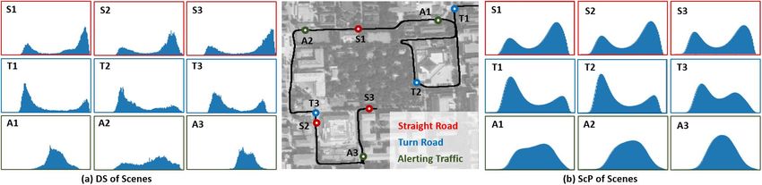
You can also read