Spectral Feature Extraction Based on the DCPCA Method
←
→
Page content transcription
If your browser does not render page correctly, please read the page content below
Publications of the Astronomical Society of Australia (PASA), Vol. 30, e24, 16 pages.

            C Astronomical Society of Australia 2013; published by Cambridge University Press.
            doi:10.1017/pas.2012.24

            Spectral Feature Extraction Based on the DCPCA Method

            BU YUDE1,5 , PAN JINGCHANG2 , JIANG BIN2 , CHEN FUQIANG3 and WEI PENG4
            1 School of Mathematical and Statistical, Shandong University, Weihai, 264209 Shandong, China
            2 School of Mechanical, Electrical and Information Engineering, Shandong University, Weihai, 264209 Shandong, China
            3 College of Electronics and Information Engineering, Tongji University, 201804 Shanghai, China
            4 Key Laboratory of Optical Astronomy, National Astronomical Observatories, Chinese Academy of Sciences, 100012 Beijing,                   China
            5 Email:   yude001@yahoo.com.cn

            (Received June 13, 2012; Accepted December 7, 2012; Online Publication February 19, 2013)

            Abstract
            In this paper, a new sparse principal component analysis (SPCA) method, called DCPCA (sparse PCA using a difference
            convex program), is introduced as a spectral feature extraction technique in astronomical data processing. Using this
            method, we successfully derive the feature lines from the spectra of cataclysmic variables. We then apply this algorithm
            to get the first 11 sparse principal components and use the support vector machine (SVM) to classify. The results show
            that the proposed method is comparable with traditional methods such as PCA+SVM.
            Keywords: astronomical instrumentation, methods and techniques – methods: analytical – methods: data analysis –
            methods: statistical

            1 INTRODUCTION                                                                          ods have been introduced to improve the interpretability of
                                                                                                    the PCs. The sparse principal component analysis (SPCA)
            Since the inherent size and dimensionality of the data given                            has been proved to be a good solution to this problem.
            by the observation such as the Sloan Digital Sky Survey                                 The SPCA attempts to give the sparse vectors, which will
            (SDSS; York et al. 2000), numerous methods have been                                    be used as PC coefficients. In sparse vectors, the compo-
            developed in order to classify the spectra in an automatic                              nents that correspond to the non-important variables will
            way. The principal component analysis (PCA) is among the                                be reduced to zero. Then, the variables which are impor-
            most widely used techniques. In Deeming (1964), the PCA                                 tant in constructing PCs will become apparent. Using this
            was first introduced to astronomical spectral data processing.                          way, the sparse PCA improves the interpretability of the
            The author investigated the application of PCA in classifying                           PCs.
            late-type giants. Connolly et al. (1995) discussed the appli-                              The SPCA method may originate from Cadima & Jol-
            cation of PCA in the classification of optical and UV galaxy                            liffe (1995), in which the authors attempted to get the
            spectra. They found that the galaxy spectral types can be                               sparse principal components (SPCs) by a simple axis ro-
            described in terms of one parameter family: the angle of the                            tation. The following works, such as sparse PCA (SPCA;
            first two eigenvectors given by PCA. They also found that                               Zou, Hastie, & Tibshirani 2006), direct approach of sparse
            the PCA projection for galaxy spectra correlates well with                              PCA (DSPCA; d’Aspremont et al. 2007) and greedy search
            star formation rate. Yip et al. (2004b), using PCA, studied                             sparse PCA (GSPCA; Moghaddam, Weiss, & Avidan 2007),
            the properties of the quasar spectra from SDSS with various                             show that the SPCA can be approached in different ways.
            redshifts.                                                                              In Sriperumbudur, Torres, & Gert (2011), the authors in-
               Schematically, PCA attempts to explain most of the vari-                             troduced a sparse PCA algorithm, which they called the
            ation in the original multivariate data by a small number of                            DCPCA (sparse PCA using a difference convex program)
            components called principal components (PCs). The PCs are                               algorithm. Using an approximation that is related to the neg-
            the linear combination of the original variables, and the PC                            ative log-likelihood of a Student’s t-distribution, in Sripe-
            coefficients (loadings) measure the importance of the cor-                              rumbudur, Torres, & Gert (2011), the authors present a solu-
            responding variables in constructing the PCs. However, if                               tion of the generalised eigenvalue problems by invoking the
            there are too many variables, we may not know which vari-                               majorisation–minimisation method. As an application of this
            ables are more important than others. In that case, the PCs                             method, a sparse PCA method called DCPCA (see Table 1) is
            may be difficult to interpret and explain. Different meth-                              proposed.
                                                                                                1

Downloaded from https://www.cambridge.org/core. IP address: 46.4.80.155, on 14 May 2021 at 12:23:48, subject to the Cambridge Core terms of use, available at https://www.cambridge.org/core/terms.
https://doi.org/10.1017/pas.2012.24
2 Bu et al.
Table 1. The algorithm of DCPCA. extraction and then applied to reduce the dimension of the
spectra to be classified. The advantage of this approach over
The algorithm of DCPCA
the PCA will then be discussed. In Section 5, we consider the
Require a A: A ࢠ b Sn + , ε > 0 and ρ > 0. effect of parameter variation and present the practical tech-
1: Choose x(0) ࢠ {c X:XT X ࣘ 1} nique about the reliable and valid applications of DCPCA.
ρ
2: ρ = log(1+ −1 ) Section 6 concludes the work.
3: repeat
4: ω(l) i = (|x(l) i | + ε)−1
5: if ρ εFeature Extraction Using DCPCA 3
This approach has been proved to be tighter than the x1 Table 2. The algorithm of
approach, see Sriperumbudur, Torres, & Gert (2011). Then, iterative.
problem (2) is equivalent to the following problem:
The algorithm of iterative
⎧ |xi |
⎫
⎨
n log 1 + ⎬
Require: a A0 ࢠ Sn +
max xT Ax − ρ lim : xT Bx ≤ 1 . (3)
x ⎩ →0 ⎭ 1. B0 ←I
i=1 log 1 + 1
2. For t = 1, . . . , r
(1) Take A←At−1
It can be approximated by the following approximate sparse
(2) Running Algorithm 1, return xt
GEV problem: (3) qt ←Bt−1 xt
⎧ |x |
⎫ (4) At ←(I − qt qT t )At−1 (I − qt qT t )
⎨ n log 1 + i ⎬
(5) Bt ←Bt−1 (I − qt qT t )
max x Ax − ρ
T
: xT Bx ≤ 1 . (4) x
x ⎩ ⎭ (6) xt ← xt
i=1 log 1 +
1
t
3. Return {x1 , . . . , xr {
Unlike problem (2), problem (4) is a continuous optimisa-
aA is the covariance matrix.
tion problem. It can be written as a difference convex (d.c.)
program, which has been well studied and can be solved
by many global optimisation algorithms (Horst & Thoai
by the M-M algorithm, a generalisation of the well-known
1999).
expectation–maximisation algorithm, the problem is finally
Let ρ = ρ/log(1 + 1 ). We can then reduce the above
solved.
problem into the following d.c. problem:
⎧
Using DCPCA, we can get the first sparse eigenvector
⎨
n of the covariance matrix A, and then obtain the following r
min τ x22 − xT (A + τ In )x − ρ log(yi + ) : (r = 1, 2, . . . , m − 1), leading eigenvectors of A through the
x,y ⎩
i=1 deflation method given in Table 2.
⎫
⎬
× xT Bx ≤ 1, −y ≤ x ≤ y (5)
⎭ 3 A BRIEF INTRODUCTION TO CATACLYSMIC
VARIABLES
by choosing an appropriate τ ࢠ R such that A + τ In ࢠ Sn +
(the set of positive semidefinite matrices of size n × n defined CVs are binary stars. The three main types of CVs are novae,
over R). Suppose dwarf novae, and magnetic CVs, each of which has various
subclasses. The canonical model of the system consists of a
n
g((x, y), (z, w)) := τ x22 − zT (A + τ In )z + ρ log( + wi ) white dwarf star and a low-mass red dwarf star, and the white
i=1 dwarf star accretes material from the red one via the accretion
n disk. Because of thermal instabilities in the accretion disk,
yi − wi
−2(x − z)T (A + τ In )z + ρ , (6) some of these systems may occasionally outburst and become
wi +
i=1 several magnitudes brighter for a few days to a few weeks at
which is the majorisation function of most.
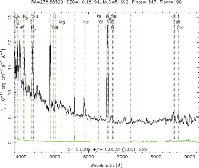
The spectra of CVs in an outburst phase have obvious
n
f (x, y) = τ x22 + ρ log( + yi ) − xT (A + τ In )x. (7) Balmer absorption lines. A typical spectrum of CVs is given
i=1 by Figure 1. The observation of 20 CVs and related objects
The solution of (7) can be obtained by the following by Li et al. presented us with the characteristics of the CVs
majorisation–minimisation (M-M) algorithm: spectra. They classified the spectra into the following three
groups (Li, Liu, & Hu 1999):
x(l+1) = arg min{τ x22 − 2xT (A + τ In )x(l)
x
n
|xi | • Spectrum with emission lines, including the hydrogen
+ ρ : xT Bx ≤ 1}, (8) Balmer emission lines, neutral helium lines, and ionised
i=1
|xi(l) | +
helium lines, sometimes Fe ii lines and C iii/N iii lines.
which is a sequence of quadratically constrained quadratic They are quiet dwarf nova or nova-like variables;
programs. As an application of this method, the DCPCA • Spectrum with the H emission lines, whose Balmer
algorithm is proposed. lines are absorption lines with emission nuclear core,
Briefly, the sparse PCA problem can be considered as a sometimes with neutral helium lines. They are dwarf
special case of the generalised eigenvector problem (GEV). nova or nova-like variables in the outburst phase;
By some approximate techniques, the GEV problem can be • Spectrum with Balmer lines, which have pure absorp-
transformed to a continuous optimisation problem (COP) tion spectra composed of helium lines, or emission nu-
which can be solved in various ways. In the DCPCA algo- clear in low quantum number of Balmer lines. They are
rithm, the COP is first formulated as a d.c. program. Then probably dwarf stars in the outburst phase.
PASA, 30, e24 (2013)
doi:10.1017/pas.2012.24
Downloaded from https://www.cambridge.org/core. IP address: 46.4.80.155, on 14 May 2021 at 12:23:48, subject to the Cambridge Core terms of use, available at https://www.cambridge.org/core/terms.
https://doi.org/10.1017/pas.2012.244 Bu et al.
1
0.9
0.8
0.7
Sparsity
0.6
0.5
0.4
0.3
0.2
0.1
0
0 1 2 3 4 5 6
ρ (× 10−4)
Figure 2. Sparsity of the first SES versus parameter ρ by using two different
Figure 1. Spectrum of a cataclysmic variable star. initial vectors x(0) = x1 and x(0) = x2 , where x1 = ( √3,522
1
, . . . , √3,522
1
)T
and x2 = ( √1,000
1
, . . . , √1,000
1
, 0, . . . , 0)T . Both x(0) satisfy (x(0) )T x(0) = 1.
The red diamond represents the result obtained by using x1 , and the blue
The observation of the CVs has a long history. Initial stud- diamond represents the result obtained by using x2 . This figure shows that the
ies concentrated on the optical part of the spectrum. Thanks to sparsity will change with the increase of ρ. Moreover, for a given sparsity,
the development of astronomical techniques and instruments, the corresponding ρ will vary with the change of the initial vector x(0) . Other
e.g., multi-fiber and multi-aperture spectrographs, adaptive x(0) will lead to a similar conclusion. For simplicity, we will not give any
optics, etc., it becomes possible for the multi-wavelength further discussion on the effect of different x(0) .
studies of the spectrum to gain the maximum information
about this binary system. From 2001 to 2006, Szkody et al.
had been using SDSS to search for CVs. These studies pro- where
vide us with a sample of 208 CVs spectra (Szkody et al. 2002,
1
n
2003, 2004, 2005, 2006, 2007), which has the statistical sig- X= X = (xi )
nificance for the following research. n i=1 i
In the following, we will first apply the DCPCA method to
and
extract the characteristic lines of these spectra of CVs. Then,
1
n
the DCPCA+SVM method will be applied to the automatic
si j = (x − xi )(xt j − x j ).
classification of CVs. The results show that this algorithm n − 1 t=1 ti
can effectively extract the spectral information of the celestial
target, which approves that the method can be applied to the Taking this covariance matrix as the input matrix of DCPCA,
automatic classification system. we will get the first SES of Sm×m . Then, using the iterative
procedure proposed in Mackey (2009) (see Table 2), we are
able to get the other r (r = 1, 2, . . . , m − 1) leading SESs.
4 EXPERIMENT Suppose that the SES Yi of length n has r non-zero ele-
ments, then the sparsity of Yi is defined as
4.1 Data preprocessing
n−r
The spectral data, each of which has 3,522 feature compo- h= .
n
nents, have been sky subtracted and flux normalised, and
In Algorithm 1 (see Table 1), there are three parameters
cover the wavelength range 3,800–9,000 Å. Suppose the
to be determined: ε, ρ, and the initial vector x(0) . In prac-
spectral data set is given by
tice, for simplicity, we set ε = 0.1 and assume x(0) =
x11 , x12 , . . . , x1m X1 ( √3522
1
, . . . , √3522
1
)T (such that (x(0) )T x(0) = 1). The param-
Xn×m = ......... = ... , eter ρ needs to be determined, since it will affect sparsity
xn1 , xn2 , . . . , xnm Xn
directly (see Figure 2). In practice, we let ρ range from min
where Xi (i = 1, . . . , n) represents a spectrum. The covariance |Ax(0) | to max |Ax(0) | with step length
matrix of Xn×m is
(max |Ax(0) | − min |Ax(0) |)/100,
1
n
Sm×m = (X − X )T (Xi − X ) = (si j ), where min |Ax(0) | and max |Ax(0) | are the minimum and max-
n − 1 i=1 i imum values of the column vector |Ax(0) |, respectively. With
PASA, 30, e24 (2013)
doi:10.1017/pas.2012.24
Downloaded from https://www.cambridge.org/core. IP address: 46.4.80.155, on 14 May 2021 at 12:23:48, subject to the Cambridge Core terms of use, available at https://www.cambridge.org/core/terms.
https://doi.org/10.1017/pas.2012.24Feature Extraction Using DCPCA 5
(a) (b)
0.045 0.15
0.04
0.1
0.035
0.03
0.05
0.025
0.02
0
0.015
0.01
−0.05
0.005
0 −0.1
4,000 5,000 6,000 7,000 8,000 9,000 4,000 5,000 6,000 7,000 8,000 9,000
Wavelength Wavelength
Figure 3. (a) Original spectrum of CVs and (b) feature lines extracted by DCPCA.
these 101 different values of ρ, we could get 101 SESs with The first three SESs, and their comparison with the corre-
different sparsity. The SESs we used in the following experi- sponding eigenspectra given by PCA, are given by Figures
ments are chosen from these ones. We find that the SES with 4–6. As we have seen from these three figures, the non-
the required sparsity lies within these SESs. The dependence essential parts of the spectra have been gradually reduced
of the sparsity on the parameter ρ is given in Figure 2. to zero by DCPCA. They illustrate the performance of the
sparse algorithm DCPCA in feature extraction. Four obvious
emission lines, i.e. Balmer and He ii lines, which we used to
identify CVs, have been derived successfully. Thus, the spec-
4.2 Feature extraction using DCPCA tral features in the SES given by DCPCA are obvious and can
PCA has been used with great success to derive the eigen- be interpreted easily. Nevertheless, as shown in Figures 4–6,
spectra for the galaxy classification system. The redshift mea- it is difficult for us to recognise the features in the PCA eigen-
surement of galaxies and QSOs has also used the eigenspec- spectra. This confirms that SES is more interpretable than
trum basis defined by a PCA of some QSO and galaxy spectra ES.
with known redshifts. In this section, the DCPCA is first ap- As we have seen, the non-essential parts of the spectra now
plied to derive the feature lines of CVs, then to get the SESs are reduced to the zero elements of SESs. However, if there
of CVs spectra, which provides a different approach to the are too many zero elements in SESs, the spectral features
feature extraction procedure. The experiment results show will disappear. Then, it is crucial for us to determine the
that this method is effective and reliable. The orientation of optimal sparsity for the SESs. The optimal sparsity should
the eigenspectra given in the figures of this section will be have the following properties: the SES with this sparsity
arbitrary. retains the features of the spectra and, at the same time, it has
the minimum number of the non-zero elements.
In order to determine the optimal value of sparsity, we plot
the eigenspectra with different sparsity and then compare
1. Feature lines extraction. In this scheme, the DCPCA
them. As shown in Figure 7, the sparsity of the eigenspectrum
is applied to derive the feature lines of CVs spectra.
between 0.95 and 0.98 is optimal. If the sparsity is below
The original spectra and the corresponding feature lines
0.95, there are still some redundant non-zero elements in the
derived by DCPCA are given by Figure 3. As we can
SES. If the sparsity is above 0.98, some important spectral
see, the spectral components around the feature lines
features will disappear.
have been extracted successfully, in the meantime, the
remaining components have been reduced to zero.
2. Feature extraction. The sample of CVs spectra data 4.3 Classification of CVs based on DCPCA
X208×3,522 we used in this scheme are the 208 spectra ob-
served in Szkody et al. (2002, 2003, 2004, 2005, 2006, 4.3.1 A review of support vector machine
2007). Let S3,522×3,522 be the corresponding covariance The SVM, which is proposed by Vapnik and his fellowships
matrix of X208×3,522 . We then apply the DCPCA algo- in 1995 (Vapnik 1995) is a machine learning algorithm based
rithm to S3,522×3,522 to get the SESs. on statistical learning theory and structural risk minimisation
PASA, 30, e24 (2013)
doi:10.1017/pas.2012.24
Downloaded from https://www.cambridge.org/core. IP address: 46.4.80.155, on 14 May 2021 at 12:23:48, subject to the Cambridge Core terms of use, available at https://www.cambridge.org/core/terms.
https://doi.org/10.1017/pas.2012.246 Bu et al.
(a) (b)
0.06 0.06
0.05 0.05
0.04 0.04
0.03 0.03
0.02 0.02
0.01 0.01
0 0
−0.01 −0.01
−0.02 −0.02
−0.03 −0.03
−0.04 −0.04
4,000 5,000 6,000 7,000 8,000 9,000 4,000 5,000 6,000 7,000 8,000 9,000
(c) (d)
0.06 0.1
0.04 0.05
0
0.02
−0.05
0
−0.1
−0.02
−0.15
−0.04
−0.2
−0.06 −0.25
4,000 5,000 6,000 7,000 8,000 9,000 4,000 5,000 6,000 7,000 8,000 9,000
Wavelength Wavelength
Figure 4. The first eigenspectra given by PCA and DCPCA. (a) The first eigenspectrum given by PCA; the first SES with sparsity (b) h = 0.0009, (c) h =
0.1911, and (d) h = 0.9609. Panels (a–d) show that the difference between eigenspectra given by PCA and DCPCA gradually becomes apparent. Panels (a)
and (b) can be considered as the same figure (the sum of their difference is less than 0.03). The differences between (a) and (c–d) are apparent. These SESs
are chosen from the 101 SESs obtained by using the method given by Section 4.1.
(Christopher 1998). It mainly deals with two-category clas- quadratic optimisation problem:
sification problems, and also regression problems. Suppose 1
that we have a training data set Minimise w · w subject to yi (w · xi + b) ≥ 1(i = 1, . . . , n).
2
D = {(xi , yi )|xi ∈ Rm , yi ∈ {−1, 1}, i = 1, . . . , n}, We transform it to the corresponding Lagrangian, by intro-
ducing a Lagrange multiplier for each constraint in the above
where xi ࢠ Rm represents the feature of the data and yi is either problem. Then, the previous constrained problem can be ex-
−1 or 1, indicating the class to which the corresponding point pressed as
xi belongs. For the linear classification problem, to classify
1 n
one group from the other more precisely, SVM finds a linear min max w · w − αi [yi (w · xi + b) − 1] = min max W.
separating hyperplane w,b αi >0 2 i=1
w,b αi >0
(9)
w·x+b=0
To solve problem (9), we compute the partial derivative of
with the maximal margin in the feature space. Mathemat- the above object function W, which leads to w = ࢣn i = 1 α i yi xi
ically, SVM finds the solution to the following convex and ࢣn i = 1 α i yi = 0. Substituting them into the above object
PASA, 30, e24 (2013)
doi:10.1017/pas.2012.24
Downloaded from https://www.cambridge.org/core. IP address: 46.4.80.155, on 14 May 2021 at 12:23:48, subject to the Cambridge Core terms of use, available at https://www.cambridge.org/core/terms.
https://doi.org/10.1017/pas.2012.24Feature Extraction Using DCPCA 7
(a) (b)
0.16 0.02
0.14 0
0.12 −0.02
0.1 −0.04
0.08 −0.06
0.06 −0.08
0.04 −0.1
0.02 −0.12
0 −0.14
−0.02 −0.16
4,000 5,000 6,000 7,000 8,000 9,000 4,000 5,000 6,000 7,000 8,000 9,000
(c) (d)
0.02 0.1
0
0
−0.02
−0.1
−0.04
−0.2
−0.06
−0.08 −0.3
−0.1
−0.4
−0.12
−0.5
−0.14
−0.6
−0.16
−0.18 −0.7
4,000 5,000 6,000 7,000 8,000 9,000 4,000 5,000 6,000 7,000 8,000 9,000
Wavelength Wavelength
Figure 5. The second eigenspectra given by PCA and DCPCA. (a) The second eigenspectrum given by PCA; the second SES with sparsity (b) h = 0, (c)
h = 0.2348, and (d) h = 0.9171. The differences between panels (a) and (b–d) are apparent. The SESs are chosen from the 101 SESs obtained by using the
method given by Section 4.1.
function, we can get the dual of the problem (9): fit the maximum–margin hyperplane in a transformed fea-
ture space. In this paper, we will use the Gaussian kernel
n
1 function
Maximise L(α) = αi − α α y y (x , x ),
2 i,j i j i j i j
i=1 x − y2
k(x, y) = exp − .
2σ 2
n
SVM has been proved to be efficient and reliable in the
subject to 0 ≤ αi ≤ C and αi yi = 0.
object classification. In our experiments, DCPCA is applied
i=1
to reduce the size of spectra from 3,522 to 3 sparse PCs and
Using the kernel trick, we can extend the previous method then SVM is used for an automatic classification. The com-
to the nonlinear classification problem (Muller et al. 2001). parison of this method with the related PCA+SVM method
The resulting algorithm is formally similar, except that ev- will then be presented.
ery dot product is replaced by a nonlinear kernel function When we apply SVM to the classification problem, the
k(x, y) = φ(x)T φ(y), where φ(x) maps x into a higher di- parameter σ in the Gaussian kernel function needs to be
mensional space. The kernel function is equivalent to the determined. In our experiments, for the sake of simplicity, we
distance between x and y measured in the higher dimen- make a priori choice of using σ = 1. We will show in Section
sional space transformed by φ. This allows the algorithm to 4.3.2 that the classification results are almost independent of
PASA, 30, e24 (2013)
doi:10.1017/pas.2012.24
Downloaded from https://www.cambridge.org/core. IP address: 46.4.80.155, on 14 May 2021 at 12:23:48, subject to the Cambridge Core terms of use, available at https://www.cambridge.org/core/terms.
https://doi.org/10.1017/pas.2012.248 Bu et al.
(a) (b)
0.08 0.02
0
0.06
−0.02
0.04
−0.04
0.02 −0.06
0 −0.08
−0.1
−0.02
−0.12
−0.04
−0.14
−0.06 −0.16
4,000 5,000 6,000 7,000 8,000 9,000 4,000 5,000 6,000 7,000 8,000 9,000
(c) (d)
0.05 0.1
0.05
0
0
−0.05
−0.05
−0.1
−0.1
−0.15
−0.15
−0.2
−0.2 −0.25
4,000 5,000 6,000 7,000 8,000 9,000 4,000 5,000 6,000 7,000 8,000 9,000
Wavelength Wavelength
Figure 6. The third eigenspectra given by PCA and DCPCA. (a) The third eigenspectrum given by PCA; (b) the third SES with sparsity (b) h = 0, (c) h
= 0.2641, and (d) h = 0.9645. The differences between panels (a) and (b–d) are apparent. The SESs are chosen from the 101 SESs obtained by using the
method given by Section 4.1.
the value of σ . Since the choice of σ has no direct influence Table 3. Information
on our conclusion, this is not discussed further. However, it of the spectral data.
is worth noting here that there is extensive literature on how
Galaxy Star QSO
to choose an appropriate kernel parameter for each particular
data set (Ishida & de Souza 2012). 1,559 3,981 1,278
4.3.2 Classification using SVM
As the PCA method has been used as a dimensionality reduc-
tion tool in spectral classification, we may wonder whether
The spectral data we used are provided by the Data Release 7
the DCPCA can be used to accomplish the same task. In this
of SDSS. The detailed information of these spectra is given in
section, the following two methods will be applied to the
Table 3. The data set is randomly divided into two equal parts:
CVs separation problem:
D1 and D2. Then, 208 CVs spectra are randomly divided into
two equal parts: C1 and C2. The data D1+C1 will be used
• DCPCA+SVM. for training and D2+C2 for testing. The final classification
• PCA+SVM. results will be represented by the classification accuracy r,
PASA, 30, e24 (2013)
doi:10.1017/pas.2012.24
Downloaded from https://www.cambridge.org/core. IP address: 46.4.80.155, on 14 May 2021 at 12:23:48, subject to the Cambridge Core terms of use, available at https://www.cambridge.org/core/terms.
https://doi.org/10.1017/pas.2012.24Feature Extraction Using DCPCA 9
(a) (b)
0.06 0.1
0.05
0.05
0.04
Sparsity = 0.00085179 Sparsity = 0.79273
0.03 0
0.02
−0.05
0.01
−0.1
0
−0.01 −0.15
−0.02
−0.2
−0.03
−0.04 −0.25
4,000 5,000 6,000 7,000 8,000 9,000 4,000 5,000 6,000 7,000 8,000 9,000
(c) (d)
0.1 0.1
0.05 0.05
Sparsity = 0.86258 Sparsity = 0.9523
0 0
−0.05 −0.05
−0.1 −0.1
−0.15 −0.15
−0.2 −0.2
−0.25 −0.25
4,000 5,000 6,000 7,000 8,000 9,000 4,000 5,000 6,000 7,000 8,000 9,000
(e) (f)
0.1 0
−0.1
0.05
Sparsity = 0.97558 −0.2
0 −0.3
−0.4
−0.05 Sparsity = 0.98495
−0.5
−0.1
−0.6
−0.15 −0.7
−0.8
−0.2
−0.9
−0.25 −1
4,000 5,000 6,000 7,000 8,000 9,000 4,000 5,000 6,000 7,000 8,000 9,000
Wavelength Wavelength
Figure 7. The first sparse eigenspectra with various sparsity. The spectral features will disappear if sparsity is above 0.98, while the redundant elements of
the spectrum have not been reduced to zero if sparsity is below 0.95.
PASA, 30, e24 (2013)
doi:10.1017/pas.2012.24
Downloaded from https://www.cambridge.org/core. IP address: 46.4.80.155, on 14 May 2021 at 12:23:48, subject to the Cambridge Core terms of use, available at https://www.cambridge.org/core/terms.
https://doi.org/10.1017/pas.2012.2410 Bu et al.
(a) (b)
0.4 0
0.3
−0.1
0.2
0.1 −0.2
0
−0.3
−0.1
−0.4
−0.2
−0.3 −0.5
−0.4
−0.6
−0.5
−0.6 −0.7
−0.8 −0.6 −0.4 −0.2 0 0.2 0.4 0.6 −0.7 −0.6 −0.5 −0.4 −0.3 −0.2 −0.1 0
Figure 8. Two-dimensional projection of 208 CV spectra given by (a) PCA and (b) DCPCA.
(a) (b)
0
0
CVs (training)
CVs (training)
non−CVs (training)
−0.1 non−CVs (training)
data3 −0.1 decision bound
CVs (test)
non−CVs (test)
−0.2 −0.2
−0.3 −0.3
SPC2
−0.4 −0.4
−0.5 −0.5
−0.6 −0.6
−0.7 −0.7
−0.7 −0.6 −0.5 −0.4 −0.3 −0.2 −0.1 0 −0.7 −0.6 −0.5 −0.4 −0.3 −0.2 −0.1 0
SPC1 SPC1
Figure 9. Result of DCPCA+SVM. SPC1 represents the first sparse principal component computed with DCPCA, and SPC2 is the second principal
component. The sparsity of the SESs which are applied to get SPC1 and SPC2 is 0.9749. The training set is represented by the red star (CVs), green
circles (non-CVs). The decision boundary of SVM is applied to classify the CVs and non-CVs in the test set. (a) CVs test sample points (blue diamond)
are superimposed to the training set. (b) Non-CVs test sample points (blue dots) are superimposed to the training set. This figure and the following figure
(Figure 11) are merely two-dimensional illustrations to show the projected spread of points. This particular configuration is not used in the classification.
which is defined by of the SES. We will show that the classification results will
not decrease with the increase of sparsity.
Nm The procedure of the experiment is given in Table 4. The
r= ,
Ns first two DCPCA-projected dimensions of the CVs spectra
data are given in Figure 8(b). The two-dimensional repre-
where Nm and Ns denote the number of correctly classified sentation of the classification result is given in Figures 9(a)
objects and the total number of objects in the test sample set, and (b). For clarity, we will show the CVs and non-CVs in
respectively. the test set in two different plots (Figures 9 a and b). We
1. DCPCA+SVM. In this scheme, the SVM is applied to also plot the decision boundary given by SVM in training.
the first three dimension data which are obtained by the first The objects of the test set located on one side of the deci-
three SESs with various sparsity. We will investigate the sion boundary will be classified as CVs, and others will be
relationship between the classification result and the sparsity classified as non-CVs. As we can see, the CVs have been
PASA, 30, e24 (2013)
doi:10.1017/pas.2012.24
Downloaded from https://www.cambridge.org/core. IP address: 46.4.80.155, on 14 May 2021 at 12:23:48, subject to the Cambridge Core terms of use, available at https://www.cambridge.org/core/terms.
https://doi.org/10.1017/pas.2012.24Feature Extraction Using DCPCA 11
Table 4. Experiment using DCPCA+SVM. 1
Classification using DCPCA+SVM 0.9
Require: Training data set A, testing data set A1 0.8
1: Use the DCPCA to find the sparse eigenspectra matrix D of A.
2: The low-dimension representation of A is given by B = AD. 0.7
3: The low-dimension representation of A1 is given by B1 = A1 D.
Accuracy
4: Input B as the training data to train the SVM. 0.6
5: Input B1 as the testing data.
6: Return the candidate of the CVs
0.5
0.4
Table 5. Experiment using PCA+SVM. 1 SPC
2 SPCS
0.3
Classification using PCA+SVM 3 SPCs
4 SPCs
0.2
Require: Training data set A, testing data set A1 0 0.2 0.4 0.6 0.8 1
1: Use the PCA to find the eigenspectra matrix P of A.
Sparsity
2: The low-dimension representation of A is given by B = AP.
3: The low-dimension representation of A1 is given by B1 = A1 P.
Figure 10. Classification accuracy versus sparsity of the SESs. It shows that
4: Input B as the training data to train the SVM.
the classification results using four SPCs, which are obtained by the first
5: Input B1 as the testing data.
four SESs, are similar to those using three SPCs. Thus, the discussion about
6: Return the candidate of the CVs
the relationship between classification results and the sparsity is limited on
the first three SESs.
generally well separated in the two-dimensional projected
space. The classification results obtained by using the first improved significantly. Thus, we limit our discussion to the
three PCs (including using 1 PC, 2 PCs, and 3 PCs), which first three SESs for clarity.
are obtained by the first three SESs with various sparsity, are 2. PCA+SVM. In this scheme, first, PCA is applied to
shown in Figure 10. From Figure 10, we find that the clas- reduce the spectral data into 1–11 dimensions, and then
sification accuracies have not decreased with the increase of the SVM method is used for automatic classification. The
sparsity. Therefore, we conclude that, while reducing most procedure of the experiment is given in Table 5. The first two
of the elements into zero, DCPCA retains the most important PCA-projected dimensions of the CVs spectra are given in
characteristics of the spectra in the SESs. Figure 8(a). The two-dimensional representation of the clas-
Four SESs with various sparsity have been used in the sification results is given in Figure 11, in which the CVs and
experiment. As shown in Figure 10, the results have not been non-CVs points in the test set are represented as Figure 9.
(a) (b)
1
1
CVs (training)
CVs (training)
non−CVs (traing)
0.8 decision bound
non−CVs (training)
0.8 decision bound
CVs (test)
non−CVs (test)
0.6
0.6
0.4
0.4
PC2
0.2
0.2
0 0
−0.2 −0.2
−0.4 −0.4
−0.8 −0.6 −0.4 −0.2 0 0.2 0.4 0.6 −0.8 −0.6 −0.4 −0.2 0 0.2 0.4 0.6
PC1 PC1
Figure 11. Result of PCA+SVM. PC1 represents the first principal component computed with PCA, and PC2 is the second principal component. The
training set is represented by the red star (CVs) and green circles (non-CVs). The decision boundary of SVM is applied to classify the CVs and non-CVs in
the test set. (a) CVs test sample points (blue diamond) are superimposed to the training set. (b) Non-CVs test sample points (blue dots) are superimposed to
the training set. This figure is merely two-dimensional illustrations to show the projected spread of points. This particular configuration is not used in the
classification.
PASA, 30, e24 (2013)
doi:10.1017/pas.2012.24
Downloaded from https://www.cambridge.org/core. IP address: 46.4.80.155, on 14 May 2021 at 12:23:48, subject to the Cambridge Core terms of use, available at https://www.cambridge.org/core/terms.
https://doi.org/10.1017/pas.2012.2412 Bu et al.
(a) (b)
1 1
0.9 0.9
0.8 1 dimension 0.8
0.7 0.7
0.6 0.6
Accuracy
0.5 0.5
0.4 0.4
2 dimensions
0.3 0.3
0.2 0.2
0.1 DCPCA 0.1 DCPCA
PCA PCA
0 0
0 0.2 0.4 0.6 0.8 1 0 0.2 0.4 0.6 0.8 1
(c) (d)
1 1
0.9 0.95
0.8 0.9
0.7 0.85
0.6 0.8
Accuracy
3 dimensions
0.5 0.75 4 dimensions
0.4 0.7
0.3 0.65
0.2 0.6
0.1 DCPCA 0.55 DCPCA
PCA PCA
0 0.5
0 0.2 0.4 0.6 0.8 1 0 0.2 0.4 0.6 0.8 1
Sparsity Sparsity
Figure 12. Classification results’ comparison between PCA+SVM and DCPCA+SVM. The dot line represents the classification accuracy based on PCA.
Classification accuracies using (a) the first SES with various sparsity, (b) the first two eigenspectra (SESs) with various sparsity, (c) the first three SESs
with various sparsity, and (d) the first four SESs with various sparsity. Panels (a–d) show that the SESs perform similar to eigenspectra in the classification,
though most of the elements in SESs are zero.
The classification accuracies for varying dimensions of fea- The results are given in Figure 13. We find that
ture vectors are given by Table 6 . when we use the optimum SESs (SES with the opti-
3. Comparison of DCPCA+SVM and PCA+SVM. In this mum sparsity), DCPCA+SVM performs better than PCA+
scheme, we will compare the performance of ES with that of SVM.
SES in classification. Figures 12 and 13 show that the performance of
First, we perform DCPCA+SVM by using the first four DCPCA+SVM is comparable with that of PCA+SVM. When
SESs with various sparsity, and then compare the perfor- we use the optimum SESs (the average sparsity is 0.9781),
mance with that of PCA+SVM. The comparison of these two DCPCA+SVM performs better than PCA+SVM. Thus, we
methods is given by Figure 12. Though the DCPCA+SVM conclude that the SESs contain significant amounts of clas-
results will vary with the increase of the sparsity, we find sification information, especially the optimum SESs. Fur-
that DCPCA+SVM has separated the CVs with great suc- thermore, both figures show that the classification accuracies
cess from other objects, and its performance is comparable using more than three SESs are not improved significantly
with that of PCA+SVM. than using the first three SESs, which is consistent with the
Second, we perform DCPCA+SVM by using the first result given in Figure 10.
11 SESs with the optimum sparsity (the average sparsity In order to minimise the influence of random factors,
is 0.9781), and then make a comparison with PCA+SVM. the experiments have been repeated 10 times, and the
PASA, 30, e24 (2013)
doi:10.1017/pas.2012.24
Downloaded from https://www.cambridge.org/core. IP address: 46.4.80.155, on 14 May 2021 at 12:23:48, subject to the Cambridge Core terms of use, available at https://www.cambridge.org/core/terms.
https://doi.org/10.1017/pas.2012.24Feature Extraction Using DCPCA 13
Table 6. Classification accuracy prove the classification accuracy significantly, as shown in
of PCA+SVM. Figures 10 and 13.
For the sparsity h of the SES, we find in Section 4.2 that
Dimension Classification accuracy
h whose value is in the range of 0.95–0.98 is optimal. To
1 0.6232 verify the conclusion, we will compare the performance
2 0.9635 of these SESs in the DCPCA+SVM experiment. Namely,
3 0.9724 the SESs with various sparsity will be applied to get the
4 0.9690
5 0.9840
sparse principal components (SPCs), which will be used in
6 0.9842 the DCPCA+SVM experiment, and in turn, the performance
7 0.9873 of these SPCs will be utilised to evaluate these SESs. The
8 0.9884 SESs are divided into three groups: the SESs with sparsity
9 0.9873 between 0.95 and 0.98 (SES1), SESs with sparsity above
10 0.9898
11 0.9914
0.98 (SES2), and SESs with sparsity lower than 0.95 (SES3).
Then, these SESs will be used in the DCPCA+SVM exper-
iment. The experiment results are shown in Figure 15. We
1
find that the classification results using SES1 are obviously
better than those using SES2 and SES3, which confirms that
0.9
the sparsity between 0.95 and 0.98 is optimal.
0.8 Despite DCPCA is reliable in extracting spectral features,
0.7
it is worth noting that it may take a long time to determine
a suitable ρ with which we can obtain a required SES. As
0.6
Accuracy
shown in Figure 2, the sparsity of the SES depends on the
0.5 value of the parameter ρ. However, using the method speci-
0.4
fied in Section 4.1, we can get the optimal SES (the sparsity
of which lies within the optimum interval) quickly. Thus,
0.3
there is no need to determine the optimum ρ (by which we
0.2 can get the optimal SES) in application. Moreover, as shown
0.1 DCPCA+SVM in Figure 2, for a given sparsity, the corresponding ρ will
PCA+SVM vary with the change of the initial vector x(0) . It makes no
0
1 2 3 4 5 6 7 8 9 10 11 sense for us to determine the optimum ρ. Though the vector
Dimension x(0) can also affect the final results, we will not discuss it
further for simplicity.
Figure 13. Classification results of DCPCA+SVM and PCA+SVM ob- Using the method proposed in Section 4.1, we can ob-
tained by using the first 11 PCs. The SPCs used in DCPCA+SVM are tain 101 different SESs corresponding to each eigenspectrum
obtained by the optimal SESs (the SESs with the sparsity lie within the
given by PCA (i.e., we can obtain 101 SESs with various
optimum interval). The average sparsity of the first 11 SESs used in experi-
ment is 0.9781. It also shows that the first three SPCs are enough for a good sparsity corresponding to the first eigenspectrum of PCA,
result, and the classification accuracies are not improved significantly if we 101 SESs with various sparsity corresponding to the second
use more than three SPCs. eigenspectrum of PCA, etc.). All SESs used in the experi-
ment and shown in figures are chosen from these SESs. It
is difficult to obtain the SESs with exactly the same spar-
classification accuracies given above are the average val- sity. For example, the sparsity of the first optimum SES is
ues. The effect of varying σ in the Gaussian kernel has been 0.9759, while that of the second one is 0.9739. In fact, we will
studied (see Figure 14). We find that the classification results not have to obtain the SESs with exactly the same sparsity.
are almost independent of the value of σ . We just need to obtain the SESs with the sparsity lying in
some interval, such as the optimum interval 0.95–0.98. Thus,
if we use more than one SES but provide only one sparsity in
5 DISCUSSION
the experiment, this sparsity is the average value. For exam-
Besides the parameters in Algorithm 1, there are three pa- ple, we used the first 11 optimum SESs in Figure 13 . Since
rameters that need to be determined in our experiment: the these optimum SESs possess different sparsity, we only pro-
σ in the Gaussian kernel, the optimal sparsity h of the SESs, vide the average sparsity 0.9781 in the figure.
and the number of the PCs we used in DCPCA+SVM. As
discussed in Section 4.3.1 and shown in Figure 14, the vari-
6 CONCLUSION
ation of σ has no direct influence on the classification result.
So, we set σ = 1 in the experiment. In the DCPCA+SVM In this paper, we first demonstrate the performance of the
experiment in Section 4.3.2, only the first three SPCs with DCPCA algorithm in the feature lines extraction by applying
various sparsity are utilised, because more SPCs will not im- it to the CVs spectra data. Then, we present an application
PASA, 30, e24 (2013)
doi:10.1017/pas.2012.24
Downloaded from https://www.cambridge.org/core. IP address: 46.4.80.155, on 14 May 2021 at 12:23:48, subject to the Cambridge Core terms of use, available at https://www.cambridge.org/core/terms.
https://doi.org/10.1017/pas.2012.2414 Bu et al.
(a) (b)
1 1
0.9 0.9
0.8 0.8
Classification accuracy
0.7
Sparsity = 0.0004 0.7
0.6 0.6 Sparsity = 0.5647
0.5 0.5
0.4 2 dimensions 0.4
0.3 0.3 2 dimensions
0.2 0.2
0.1 0.1
0 0
0 0.5 1 1.5 2 0 0.5 1 1.5 2
(c) (d)
1 1
0.9 0.9
0.8 0.8
Classification accuracy
0.7 0.7
0.6 Sparsity = 0.9299 0.6
Sparsity = 0.9848
0.5 0.5
0.4 0.4
2 dimensions 2 dimensions
0.3 0.3
0.2 0.2
0.1 0.1
0 0
0 0.5 1 1.5 2 0 0.5 1 1.5 2
σ σ
Figure 14. Classification results of SVM by using first two SESs with various sparsity versus σ in the Gaussian kernel. Sparsity of the first two SESs is
(a) 0.004, (b) 0.5647, (c) 0.9299, and (d) 0.9848. Panels (a–d) show that the classification results are almost independent of σ . The results of using other
numbers of SESs are similar.
of this algorithm in the classification of CVs spectra. In the are more interpretable. Thus, the spectral feature of
classification experiments, we first use the DCPCA to reduce CVs can be well described by the SES whose number
the dimension of the spectra, and then use SVM to clas- of non-zero elements is dramatically smaller than the
sify the CVs from other objects. The result comparing with number usually considered necessary.
the traditional PCA+SVM method shows that the reduction 2. Changing σ in Gaussian has no direct influence on our
of the number of features used by classifier does not neces- conclusion.
sarily lead to a deterioration of the separation rate. Compared 3. The sparsity of SESs between 0.95 and 0.98 is opti-
with PCA, the sparse PCA method has not been widely ap- mum.
plied in the spectral data processing. Nonetheless, the demon- 4. When we use SESs with the optimum sparsity (the av-
strations given here have shown the perspective of the sparse erage sparsity is 0.9781), DCPCA+SVM will perform
PCA method in this route. We find that better than PCA+SVM.
5. The parameter ρ has a direct influence on the sparsity of
SES. However, it is not necessary for us to determine the
optimum ρ. Using the method given in Section 4.1, we
1. DCPCA is reliable in extracting the feature of spectra. can get the optimal SES without any prior knowledge
Compared with the eigenspectra given by PCA, SESs of the optimal ρ.
PASA, 30, e24 (2013)
doi:10.1017/pas.2012.24
Downloaded from https://www.cambridge.org/core. IP address: 46.4.80.155, on 14 May 2021 at 12:23:48, subject to the Cambridge Core terms of use, available at https://www.cambridge.org/core/terms.
https://doi.org/10.1017/pas.2012.24Feature Extraction Using DCPCA 15
(a) (b)
1 1
0.98 0.9
0.96 0.8
0.94
0.7
Accuracy
0.92
0.6
0.9
0.5
0.88
0.4
0.86
0.84 0.3
SPC1+SVM SPC1+SVM
SPC2+SVM SPC3+SVM
0.82 0.2
0.95 0.96 0.97 0.98 0.99 1 0 0.2 0.4 0.6 0.8 1
Sparsity Sparsity
Figure 15. Classification accuracy versus sparsity. The SESs are divided into three groups: SESs with sparsity between 0.95 and 0.98 (SES1), SESs with
sparsity above 0.98 (SES2), and SESs with sparsity below 0.95 (SES3). Then these SESs are utilised to get the SPC groups: SPC1, SPC2, and SPC3.
These SPCs will then be used in the DCPCA+SVM experiment as in Section 4.3.2. (a) The result of SPC1+SVM versus the result of SPC2+SVM, and (b)
the result of SPC3+SVM versus the average result of SPC1+SVM. Panel (a) shows that when the sparsity is above 0.98, the classification result will be
unstable. Panels (a) and (b) show that the classification results using SPC1 are significantly better than those using SPC2 and SPC3. It implies that SES1
performs better than SES2 and SES3 in the classification. For the sake of simplicity, we use the first SPC in the classification. The classification results of
using other numbers of SPCs are similar.
ACKNOWLEDGMENTS Sriperumbudur, B. K., Torres, D. A., & Lankriet, G. R. G. 2011,
Mach. Learn., 85, 3
We thank the referee for a thorough reading and valuable comments.
Szkody, P., et al. 2002, AJ, 123, 430
This work is supported by the National Natural Science Foundation
Szkody, P., et al. 2003, AJ, 583, 430
of China (grants 10973021 and 11078013).
Szkody, P., et al. 2004, AJ, 128, 1882
Szkody, P., et al. 2005, AJ, 129, 2386
Szkody, P., et al. 2006, AJ, 131, 973
REFERENCES Szkody, P., et al. 2007, AJ, 134, 185
Weaver, W. B., & Torres-Dodgen, A. V. 1997, ApJ, 487, 847
Burges, C. J. C. 1998, Data Min. Knowl. Disc., 2, 121
Vapnik, V. 1995, The Nature of Statistical Learning theory (New
Cadima, J., & Jolliffe, I. T. 1995, J. Appl. Stat., 22, 203
York: Springer-Verlag)
Connolly, A. J., Szalay, A. S., Bershady, M. A., Kinney, A. L., &
Yip, C. W., et al. 2004b, AJ, 128, 2603
Calzetti, D. 1995, AJ, 110, 1071
York, D. G., et al. 2000, AJ, 120, 1579
d’Aspremont, A., EI Ghaoui, L., Jordan, M. I., & Lanckriet, G. R.
Zhao, R., Hu, Z., & Zhao, Y. 2005, Spectrosc. Spect. Anal., 25, 153
G. 2007, SIAM Rev., 49, 434
Zhao, R., Wang, F., Luo, A., & Zhan, Y. 2009, Spectrosc. Spect.
Deeming, T. J. 1964, MNRAS, 127, 493
Anal., 29, 2010
Gao, D., Zhang, Y.-x., & Zhao, Y.-h. 2008, MNRAS, 386,
Zou, H., Hastie, T., & Tibshirani, R. 2006, J. Comput. Graph. Stat.,
1417
15, 265
Horst, R., & Thoai, N. V. 1999, J. Optim. Theory Appl.,
103, 1
Ishida, E. E. O., & de Souza, R. S. 2012, arXiv:1201.6676 APPENDIX: PRINCIPAL COMPONENT
Li, Z., Liu, W., & Hu, J. 1999, AcASn, 40, 1 ANALYSIS
Liu, R., Liu, S., & Zhao, R. 2006, Spectrosc. Spect. Anal., 26,
583 Consider a data set
Mackey, L. 2009, in Advances in Neural Information Processing
S = ( fi j )m×n ,
Systems, ed. D. Koller, D. Schuurmans, Y. Bengio, & L. Bottou
(Vol. 21; Cambridge: MIT Press), 1017 the ith data point of which is
Moghaddam, B., Weiss, Y., & Avidan, S. 2007, in Advances in Neu-
ral Information Processing Systems ed. B. Scholkopf, J. Platt, ( fi1 , ..., fin ).
T. Hoffman (Vol. 19; Cambridge: MIT Press), 915 m
Let f q = m1 i=1 fiq and σ q be the mean and standard deviation of
Muller, K. R., Mika, S., Rätsch, G., Tsuda, K., and Schölkopf, B. the qth random variable fq , respectively. Suppose that
2001, IEEE Trans. Neural Netw., 12, 181
Singh, H. P., Gulati, R. K., & Gupta, R. 1998, MNRAS, 295, 312 Xi = (xi1 , . . . , xin )(i = 1, . . . , m),
PASA, 30, e24 (2013)
doi:10.1017/pas.2012.24
Downloaded from https://www.cambridge.org/core. IP address: 46.4.80.155, on 14 May 2021 at 12:23:48, subject to the Cambridge Core terms of use, available at https://www.cambridge.org/core/terms.
https://doi.org/10.1017/pas.2012.2416 Bu et al.
where xi j = ( fi j − f j )/σ j and then Ba1 is the projection of the standardised data set on a1 . We can
prove that the variance of Ba1 is
B = (X1T , . . . , XmT )T .
aT1 BT Ba1 = aT1 Ca1 .
Then we can show that
Our goal is to maximise this value under the constraint aT 1 a1 = 1.
m
C=B B= T
XiT Xi = (C jk )n×n , Let λmax be the largest eigenvalue of C. According to the Rayleigh–
i=1 Ritz theorem, a1 can be obtained by solving
where Cjk = ࢣm i = 1 xij xik is the correlation matrix. Our goal is to Ca1 = λmax a1 .
find a normalised vector
Then, a1 is the unitary eigenvector corresponding to λmax . Briefly,
a1 = (a11 , a12 , . . . , a1n )T to get the first component that accounts for the largest variance of
the data, we just need to get the unitary eigenvector of the corre-
such that the projection of the standardised data on a1 has the
lation matrix C that corresponding to the largest eigenvalue of C.
maximum variance. Since the projection of the ith data point Xi on
Similarly, to give the second component that is orthogonal to the
a1 (the first principal component of Xi ) is
first component and accounts for the second largest variance of the
n data, we just need to get the unitary eigenvector that corresponds
Xi a1 = xik a1k , to the second largest eigenvalue of C. The subsequent components
k=1 can be obtained in the same way.
PASA, 30, e24 (2013)
doi:10.1017/pas.2012.24
Downloaded from https://www.cambridge.org/core. IP address: 46.4.80.155, on 14 May 2021 at 12:23:48, subject to the Cambridge Core terms of use, available at https://www.cambridge.org/core/terms.
https://doi.org/10.1017/pas.2012.24You can also read