Comparison Between Linear and Non-linear Variable Selection Methods with Applications to Spectroscopic (UV-Vis/NIR) Data
←
→
Page content transcription
If your browser does not render page correctly, please read the page content below
Chiang Mai J. Sci. 2020; 47(1) : 160-174
               http://epg.science.cmu.ac.th/ejournal/
               Contributed Paper

Comparison Between Linear and Non-linear Variable
Selection Methods with Applications to Spectroscopic
(UV-Vis/NIR) Data
Chanida Krongchai [a], Sakunna Wongsaipun [a], Sujitra Funsueb [a], Parichat Theanjumpol [b,c],
Jaroon Jakmunee [a,d] and Sila Kittiwachana*[a,e]
[a] Department of Chemistry, Faculty of Science, Chiang Mai University, Chiang Mai 50200, Thailand.
[b] Postharvest Technology Research Center, Faculty of Agriculture, Chiang Mai University, Chiang Mai 50200,
   Thailand.
[c] Postharvest Technology Innovation Center, Office of the Higher Education Commission, Bangkok 10400, Thailand.
[d] Institute for Science and Technology Research and Development, Chiang Mai University, Chiang Mai 50200,
   Thailand.
[e] Environmental Science Research Center, Faculty of Science, Chiang Mai University, Chiang Mai 50200, Thailand.
*Author for correspondence; e-mail: silacmu@gmail.com
                                                                                     Received: 14 January 2019
                                                                                   Revised: 11 September 2019
                                                                                  Accepted: 16 September 2019

A BSTRACT
      		 Variable selection aims to identify important parameters in relation to predicted responses.
Selection outcomes of the important variables could be different depending on the methods used. In
this research, the important variables identified using linear and non-linear variable selection methods
based on partial least squares-variable important in prediction (PLS-VIP) and self organizing map-
discrimination index (SOM-DI) were compared. Two datasets, near-infrared (NIR) spectra of adulterated
Thai Jasmine rice and ultraviolet-visible (UV-Vis) spectra of food colorant mixtures were used for
the demonstration. The advantages and disadvantages for the use of the different algorithms were
compared and discussed. For the NIR data, the calibration model using supervised self organizing map
(SSOM) offered better prediction results and the SOM-DI variable selection method identified the
spectral changes in NIR overtone regions as significance. On the other hand, PLS calibration model
resulted in higher predictive errors while the PLS-VIP variable selection captured variation from the
visible region between 664 nm and 884 nm. Using the UV-Vis data, PLS appeared to put attention
on only the highest absorbance region of the peak maximum absorbance. In contrast, SSOM model
highlighted the variation around the isosbestic spectral regions between the mixture components.
The drawback for the use of a mixture design to construct the calibration models, leading to wrong
interpretation of the important variables, was also discussed.

Keywords: variable selection, multivariate calibration, partial least squares (PLS), self organizing map
(SOM), spectral data analysis
Chiang Mai J. Sci. 2020; 47(1)                                                                          161

1. I NTRODUCTION
      Spectroscopic measurements especially             calibration techniques can deal with a large number
ultraviolet-visible (UV-Vis) and near-infrared (NIR)    of variables dataset. However, there are some
have been increasingly used as analytical tools in      benefits if the number of predictive variables is
various field such as clinical chemistry, process       reduced. This is because not all the variables are
monitoring, food, agriculture and environmental         useful or contain informative variation for the
science [1-4]. These spectroscopic measurements         prediction models. The detected absorbance at
are based on the similar principle where the            baseline may be irrelevant or represent only noise.
interaction between the electromagnetic light           In addition, a measurement at one wavelength
radiation and analyst sample is detected. The           can be correlated to the measurement of the
difference is that UV-Vis detects the absorption        wavelengths nearby or they behave similarly.
corresponding to the electronic transitions of the      The similar trends in the measurement variables
electrons in an atom or molecule, whereas the           cause an overly complexity in data and could
absorption of NIR is as a result of the overtones       dramatically reduce the predictive performance
or combinations of the chemical functional groups       due to multicollinear problem [5]. Therefore, it is
originating in the infrared (IR) region. These          advised that suitable variable selection is performed
measurement techniques gained advantages over           prior to the construction of a calibration model.
other analytical techniques because the sample               Variable selection can be used to identify
detection can be operated quickly without or less       variables (wavelengths) that contribute useful
sample pretreatment. Using different detection          information (in this case the response), or it
modes such as transmittance, reflectance and            aims to evaluate the importance of the measured
interaction, these spectroscopic measurements can       parameters. In general, chemometric techniques,
be practical for samples that are either liquid or      used for classification or regression, could be
solid. By modern scanning instruments, UV-Vis           categorized into two major groups based on
and NIR can generate a large number of variables.       the nature of the algorithms; linear and non-
For example, a measurement of NIR could yield           linear methods [6]. At the present time, many
1701 spectral points or variables corresponding to      variable selection methods have been proposed
the absorbance in the region of 700-2400 nm at          and most of them are a generalized form their
1 nm interval. For that reason, sophisticated data      related predictive models. Partial least squares-
analysis techniques are required, and the predictive    variable important in prediction (PLS-VIP),
results should be obtained from multivariate            partial least squares-selectivity ratio (PLS-SR) and
analysis of available spectra rather than a single      PLS coefficients, are among the most common
observed variable or a single spectrum of an            variable selections which are based on the partial
individual sample.                                      least squares (PLS) regression. These methods
      Multivariate calibration aims to investigate a    expect that the significant variables linearly affect
relationship between predictive (X) and response        the change in variation of response. Unlike
(c) variables. The predictive variables are data that   PLS, self organizing map (SOM) is a non-linear
can be directly measured from samples. On the           method. This model does not expect that data
other hand, the response variables are information      follow multivariate normal distribution or that
which cannot be directly obtained from the              mathematical equations are required to explain the
measurement. This relationship information              characteristic structure of the model. Compared
between the two data blocks can be then used            to the other non-linear prediction such as artificial
to establish calibration model for prediction of        neural network (ANN) and support vector machine
unknown samples. In general, most multivariate          (SVM), SOM has an ability to display the internal
162 Chiang Mai J. Sci. 2020; 47(1)
structure of the model using some visualization constructing the calibration model was discussed.
methods such as component planes, supervised The advantages and disadvantages of applying
color shading and U-matrix [7]. Therefore, it is these two methods were reported.
possible to investigate the non-linear behavior
in relation to the predictive response. Recently, 2. M ATERIALS AND METHODS
the development of a variable selection index, 2.1 Spectroscopic Data
called self organizing map-discrimination index 2.1.1 NIR of adulterated rice
(SOM-DI), were proposed [8]. This index could The rice samples were purchased from a
be used to evaluate the variable significance in local department store. Two rice varieties were
addition the visualization of the non-linear behavior used including Khao Dawk Mali 105 (KDML105)
from the component planes. For spectral analysis, and Chai Nat 1 (CN1) white rice. The quality of
linear and non-linear calibrations could result in the rice samples was certified by ISO 9001:2008
different predictive performance. Consequently, standard with good manufacturing practice (GMP).
the identification of the important variables could To synthetically generate adulterated KDML105
be different. This led to a possible variety in the rice samples, the KDML105 rice was blended
interpretation and conclusion. with the CN1 rice where the concentrations of
This research reported the comparison of linear the mixed rice samples were ranged from 0.0
and non-linear variable selections for identifying %w/w to 100.0 %w/w with the increment of 5
important wavelengths in spectral analysis. PLS-VIP %w/w. After mixing, the samples were maintained
and SOM-DI were used to represent the linear in a controlled temperature room at 25 °C for at
and non-linear variable selections, respectively. least 6 hours to stabilize the sample temperature.
Two datasets including UV-Vis of food colorant The NIR spectra were recorded using FOSS
mixtures and NIR of adulterated Khao Dawk Mali NIR DS2500 (FOSS NIR system, USA) from
105 (KDML105) rice were used to demonstrate 400 - 2500 nm at 0.5 nm resolution. Each sample
the model characteristics. The UV-Vis dataset was measured three times and the recorded spectra
was used to demonstrate the performance of were averaged. The NIR spectra were separated
the variable selection methods when dealing into two datasets where the samples adulterated
with samples with multi-components or there at 0, 10, 20, …, 100% w/w were used as training
were several analytes at different concentration samples and the rests were used as test samples.
combined in samples. KDML105 is a well-known The recorded NIR data were exported to Matlab
Thai jasmine rice variety which is famous for program (MATLAB V7.0, The Math Works Inc.,
its present fragrant and delicious texture when Natick) for further data calculation.
cooked. The price of KDML105 is relatively
expensive and therefore it is often blended with 2.1.2 UV-Vis spectra of food colorants
some other cheaper non-fragrant rice causing This dataset was used to demonstrate the
adulteration. To comply with the labelling law, the performance of the variable selection methods
adulteration level should be clearly clarified. The when dealing with samples with multi-components
presence of the substitution or other blending or there were several analytes at different
rice more than the regulation reveals deliberate concentration combined in samples. Three food
substitution, and this will be illegal under the colorants, Carmoisine, Tartrazine and Brilliant
food labelling rules. The effect of non-linearity blue FCF representing red, yellow and blue
in data on the predictive performance of the colors, were prepared from commercial grade
calibration models was reported. A problem of chemicals. The spectrum of each food colorant
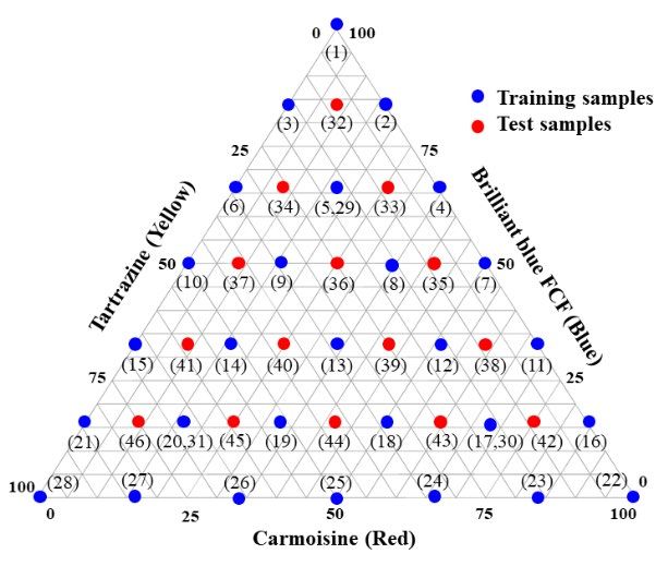
sample permutation in a mixture design when was shown in Figure 1(A). The concentrationsChiang Mai J. Sci. 2020; 47(1) 163
450
451
Carmoisine
3 Tartrazine
Brilliant blue FCF
2.5
Absorbance
2
1.5
1
0.5
0
350 400 450 500 550 600 650 700 750 800
Wavelength (nm)
(A) (B)
452
Figure 1. (A) The spectrum of each food colorant and (B) a three-component diagram model by
453 Figure 1. (A) The spectrum of each food colorant and (B) a three-component diagram model by
mixture design used to prepare the food colorant samples. The model consisted of 43 samples indicated
454 mixture design used to prepare the food colorant samples. The model consisted of 43 samples
455 using the numbers
indicated in numbers
using the parenthesis.
in parenthesis.
456
457 of the mixing samples were prepared following a data is maximized, PLS, in most cases, provides
mixture design with three components as shown satisfactory predictive results [11]. Several algorithms
458 in Figure 1(B) resulting in a total of 43 samples of PLS calculations have been reported and
459 [9]. Twenty-eight samples were used as training PLS1, proposed by Geladi and Kowalski [9-11],
samples labeled using blue circles in Figure 1(B) was used in this research. The construction of
460
and the rests were used as test samples using red PLS1 is as follows:
461 circles. Each of the samples were prepared from
462 the same solution stocks in DI water to eliminate X = TP + E
the variation form the food colorant impurity.
463 The mixing samples were measured using UV-Vis c = uq + f
464 spectrometer (GENESYS 10S UV-Vis, Thermo
Scientific, USA) ranging from 350 nm to 850 nm Firstly, X with I samples and J variables, is
465
with a resolution of 1 nm. decomposed into X-scores (T) and X-loadings (P).
466 At the same time, c is the product approximation
467 2.2 Calibration and Variable Selection Methods of u and c-loadings (q). Then, the correlation
2.2.1 Partial least squares (PLS) and partial between X and c is expressed by:
468
least squares-variable important in prediction
469 (PLS-VIP) u = bt
Partial least squares (PLS) is among the most
470
common linear regression method in multivariate When b is a regression coefficient vector
471 data analysis [10]. Based on non-linear iterative with size J x 1 and the estimation of b can be
partial least squares (NIPALS) algorithm, PLS calculated as:
captures the variation from both predictive and
response data and simultaneously then used b = Wq
for constructing a calibration model. Since the
covariance between the predictive and response164 Chiang Mai J. Sci. 2020; 47(1)
Where W is a normalized PLS weight matrix. set of square or hexagonal units. Using iterative
In this work the optimum number of latent learning process [20], the trained map of SOM
variables (LVs) were defined using bootstrap adapts itself so that the training samples are
algorithm [12]. located as far as possible from each other where
Partial least squares-variable important in the aim is to maintain the topological structure
prediction (PLS-VIP) was first reported by Wold of the training samples. At the beginning, SOM
et al. [13]. The variable selection parameter has was used as unsupervised model where only the
been extensively used in various researches such as predictive data was used for constructing the
chemistry [14], agriculture [15], medicine [16] and model. However, SOM can be used as supervised
engineering [17]. The VIP score summarize the model where the response data was given during
influence of each of X variables which considers the learning process as demonstrated in Figure 2.
the amount of explained y variance in each LV By allowing the response data to be associated in
(the number of PCs used in PLS modelling). The the learning process, it is possible to adopt SOM
VIP scores provide a measurement of useful to for classification and calibration purposes. For
selected which variables are contributed the most example, supervised SOM was used to predict
to the c response. The PLS-VIP for the jth variable the retention time of chromatographic analysis
is calculated as follows: based on quantitative structure–activity relationship
(QSAR) data [21].
M
In addition to the classification and calibration
∑w 2
jm .SSYm . J models, it is possible to investigate the importance
VIPj = m =1 of the studied variable from the SOM training
SSYtotal .M map. The extended used of SOM for variable
selection and called the proposed algorithm as self
and SSYtotal = b 2T ′T organizing map-discrimination index (SOM-DI)
was demonstrated [8]. The idea was to see if
Where wjm is the weight value for the jth the component plane profiles and the response
variable and the mth component. SSYm is the plane were alike. This can be done by calculating
sum of squares of explained variance for the mth the correlation between the response plane and
component. SSYtotal is the total sum of squares each of the variable component plane of the
explained of the dependent variable, and M is the trained map after appropriate data scaling. The
total number of components. VIPj is a measure component planes which are strongly associated
of the contribution of each variable according to with the response will have larger coefficient values.
the variance explained by each PLS component The calculation of SOM-DI and the important
were w2jm represents the importance of the jth parameters set for the supervised SOM have been
variable [18]. described in detail in report of Lloyd et al. and
Krongchai et al. [8 and 22].
2.2.2 Self organizing map (SOM) and self
organizing map-discrimination index (SOM-DI) 2.3 Assessment of Model Predictive Performance
Self organizing map (SOM) or Kohonen To evaluate the predictive performance of
network is one type of non-linear learning models the chemometric models, various model statistics
[19]. Unlike principal component analysis (PCA) including root mean square error of calibration
that clusters samples into an orthogonal space of (RMSEC), root mean square error of prediction
the first few principal components (PCs), SOM (RMSEP), cross-validated explained variance of
organizes samples into a map consisting of a training (R2) and test (Q2) sets and ratio of RMSEPChiang Mai J. Sci. 2020; 47(1) 165
Figure 2. A schematic diagram showing a SOM model with a size of P × Q. The data characterizes
by J variables and two class memberships.
and RMSEC (RP/Auto) were calculated [23]. this ratio is close to 1, this indicates a stability of
RMSEC is the average difference between model when some training samples are removed
predicted ( ĉi ) and expected ( ci ) response values from the modeling or the model is tested with
in auto-prediction mode and can be calculated as: unknown samples [23]. To highlight the scope of
this research, the spectral data were tested with
various data pretreatment such as standard normal
∑i =1 (cˆi − ci ) 2
N
RMSEC = variate (SNV), multiplicative scatter correction
N −1
(MSC), normalization, and centering [24]. The
where N is the number of samples. Using models with the best predictive results were
RMSEC, the establish model is tested directly on reported. The computations of PLS, PLS-VIP,
the calibration data or training samples, thus it supervised SOM and SOM-DI were carried
is an internal validation or auto-predictive mode. out using in-house scripts in Matlab (2010, The
On the other hand, RMSEP calculates the error MathWorks, Natick, MA).
of the predicted response values ( ĉi ) of the test
samples. 3. R ESULTS AND DISCUSSIONS
The cross-validated explained variance of 3.1 NIR and UV-Vis Datasets
the model was calculated by: NIR spectra of the rice samples and the
corresponding PCA are presented in Figure 3(A)
N
∑ (cˆ − c )i i
2 and 3(B), respectively. From the NIR spectra, the
2
Q =1− i =1
N
rice samples had similar pattern where the shapes
∑ (c − c ) i
2
of the NIR spectra were nearly identical. In this
i =1
situation, it was not easy to recognize the difference
If the predicted response values ( ĉi ) are between the samples from the investigation of the
test samples, this correlation index implies the raw spectra. However, when the data was visualized
error in test mode (Q2). Normally, the values of using the first two PCs, it was possible to observe
2 2
R and Q as close as possible to 1.0 are expected the change in the KDML105 rice samples when
and imply the greater degree of variation within mixed with the different amount of the white rice.
the data modelled by the calibration model. In Figure 3(B), the rice samples were scattered
The ratio of RMSEP and RMSEC (RP/Auto) was across the PCA space where the mixing levels
calculated to indicate the model robustness. If increased from the top to the bottom along PC2.166 Chiang Mai J. Sci. 2020; 47(1)
0.8
1.6 15
5
0.6 10
0
1.4 25
0.4
35
45 20
1.2
0.2 30
Absorbance
40 55
1 0 Trainging samples
50
PC2
Test samples
-0.2 60
0.8 65 85
-0.4 80
75
0.6 70
-0.6
90
0.4 -0.8
100 95
-1
400 600 800 1000 1200 1400 1600 1800 2000 2200 2400 -64.799 -64.798 -64.797 -64.796 -64.795 -64.794 -64.793 -64.792
Wavelength (nm) PC1
(A) (B)
495
Figure 3. (A) NIR spectra of the rice samples and (B) PCA score plot of PC1 against PC2 of the NIR
496 Figure 3. (A) NIR spectra of the rice samples and (B) PCA score plot of PC1 against PC2 of the
spectra after SNV treatment and the samples were labeled according to the percentage of KDML105.
497 NIR spectra after SNV treatment and the samples were labeled according to the percentage of
498 KDML105.
499 On the other hand, the change in variation on the cluster (the samples labeled as 1, 22 and 28)
500 PC1 was rather complicated. The samples having where the mixture samples having more than
different adulteration levels possessed similar score one component were placed in the middle of the
501
values of PC1. For example, the samples with cluster as presented in Figure 4(B).
502 10% and 90% have nearly the same PC1 score
503 values the middle of the PC1 axis. This implied 3.2 Variable Selection for the NIR Dataset of
that the NIR data has non-linear characteristics Adulterated Rice
504
in nature and multivariate analysis should be used The important variables identified using
505 to process data. PLS-VIP and SOM-DI are illustrated in Figure 5(A)
506 Figure 4(A) shows the UV-Vis spectra of and 5(B), respectively. The significant variables
the food colorant samples. It can be seen that the from both selection methods were not identical
507
samples were characterized by three overlapping meaning that they utilized the data from different
508 peaks with the λmax at 426 nm, 516 nm and 630 parts of the NIR for predicting the adulteration
509 nm, respectively, representing the absorbance of level. In Figure 5(A), PLS-VIP seemed to capture
the yellow, red and blue food colorants. The PCA the variation in the region of long visible light
510
model of the UV-Vis spectral data is presented in (664-884 nm). This indicated that the PLS-based
511 Figure 4(B). The characteristic pattern in the PCA model was sensitive toward the change in sample
512 structure of the UV-Vis data was quite different color. The variation in the sample color could be
from that of the NIR data. In the UV-Vis spectra, due to that the grain characteristics of KDML105
513
there were three components in the mixing samples was less opaque and relatively clearer than that
514 and their compositions were varied according to of CN1 white rice. Although the grain color of
515 the three-component mixture design. The detected both KDML105 and CN1 were not obviously
peaks allowed to be overlapped with different different when observed using naked eyes, the
ratios to provide the variation for quantitative spectrophotometer could be more effectively
analysis purpose. As a result, the samples in the detect the color difference. The absorbance was
PCA were clustered into one region. Each of the linearly changed with the increase of the KDML105
samples of the pure color component (100% of composition.
red, yellow and blue) was located at the edge ofChiang Mai J. Sci. 2020; 47(1) 167
40
3.5 22
Trainging samples
30 Test samples 23
3 24 16
20 30 42
2.5 18 17 11
26 25
10 38
43
Absorbance
28 19 12
20 44
2 27
40 45 39
PC2
0
46 31 13 7
8 35
1.5 14 9 36 4
-10 21 41
15 5 33
10 2 29
1 6 34 37
-20
32
3
0.5 -30 1
0 -40
350 400 450 500 550 600 650 700 750 800 -70 -60 -50 -40 -30 -20 -10 0 10 20 30
Wavelength (nm) PC1
(A) (B)
Figure
516Figure 4. (A)
4. (A) Visible
Visible spectra
spectra of of
thethefood
foodcolorant
colorantsamples
samplesand
and (B)
(B) PCA
PCA score
score plot
plotof
ofPC1
PC1 against
517PC2against PC2 of the visible
of the visible spectra. spectra.
1.6 1.6
1.4 1.4
1.2 1.2
1 1
Absorbance
Absorbance
0.8 0.8
0.6 0.6
0.4 0.4
0.2 0.2
0 0
400 600 800 1000 1200 1400 1600 1800 2000 2200 2400 400 600 800 1000 1200 1400 1600 1800 2000 2200 2400
Wavelength (nm) Wavelength (nm)
(A) (B)
Figure 5. Variable selection results of the NIR dataset using (A) PLS-VIP and (B) SOM-DI. The
Figure 5. Variable selection results of the NIR dataset using (A) PLS-VIP and (B) SOM-DI. The
wavelengths
wavelengthsidentified as significance
identified were
as significance highlighted
were highlightedusing
usingvertical
vertical closed and dotted
closed and dottedred
red lines,
respectively, for PLS-VIP and SOM-DI.
lines, respectively, for PLS-VIP and SOM-DI.
On the other hand, SOM-DI shown in Figure The predictive results using PLS and supervised
5(B) identified the characteristic NIR bands of SOM before and after the variable selection are
water (1,400 nm and 1,900 nm), OH (1,600 nm) summarized in Table 1. In this case, the predictive
and CH (1,700-1,800 nm) bonds, respectively, as performance of the PLS model clearly improved
importance [25]. These NIR regions corresponded where the RMSEP was reduced from 10.97 to
to moisture and starch molecules of grains 5.206. In addition, the error in prediction of each
implying that KDML105 has different moisture sample was reduced resulting in the higher Q2.
content and ratio of starch molecules compared The samples placed closer to the regression line
to the CN1 white rice. It was possible that the (Figure 6(B)) when compared to the correlation
changed of water, OH and CH bond signals graph of the prediction model using the whole
related to adulteration in the fragrant rice [26]. variables (Figure 6(A)). The ratio between RMSEP168 Chiang Mai J. Sci. 2020; 47(1)
Table 1. Predictive results of the NIR and ultraviolet-visible dataset using PLS and supervised SOM
before and after variable selection methods.
Full spectra
Data Methods Total variables RMSEC R2 RMSEP Q2 RP/Auto
PLS 4200 2.143 0.995 10.97 0.854 5.120
NIR
SOM 4200 1.795 0.997 3.222 0.987 1.795
PLS 451 0.0154 1.00 0.0270 0.999 1.753
UV-Vis
SOM 451 0.0548 0.999 0.0848 0.994 1.547
Selected variables
PLS-VIP 478 3.697 0.986 5.206 0.967 1.408
NIR
SOM-DI 430 3.189 0.988 2.230 0.981 1.147
PLS-VIP 44 0.015 1.00 0.0237 0.999 1.539
UV-Vis
SOM-DI 45 0.149 0.989 0.4481 0.820 3.013
(A) (B)
(C) (D)
Figure 6. Correlation
Figure graphs
6. Correlation graphsbetween
betweenexpected
expectedand
and predicted concentrationofofKDML105
predicted concentration KDML105 in the
in the
mixing ricerice
mixing samples. (A)(A)
samples. andand
(B)(B)
areare
thetheprediction
predictionusing
using PLS
PLS before and
andafter
afterthe
thevariables
variableswere
were
screened
screened by by PLS-VIP.
PLS-VIP. (C)(C)
andand (D)are
(D) arethe
theprediction
prediction using supervised
supervisedSOM
SOMbefore
beforeand after
and thethe
after
variables
variables werewere screened
screened by SOM-DI.
by SOM-DI.Chiang Mai J. Sci. 2020; 47(1) 169
and RMSEC was also reduced confirming that the based on the regression model. According to
model robustness was improved. If this parameter the assumption that the predicted response was
is close to 1, this informs that the models is not linearly changed. The predictive performance
prone to overfitting problem and the predictive of SOM could be improved by increasing the
performance of the training and test samples can number of the training samples. Since there were
be comparable. three components mixing in the samples, three
The predictive accuracy of the supervised different PLS1 models were established for each
SOM was slightly improved after the variables of the color components. Figure 7(A), 7(C) and
were screened by the SOM-DI selection. In this 7(E) show the important variables identified using
study case, SOM as a non-linear prediction still PLS-VIP for Carmoisine, Tartrazine and Brilliant
provided better predictive results when compared blue FCF food colorants. The correlation graphs
to the PLS model with the RMSEP value of 3.222 of the expected and predicted concentrations
and 2.230, for the prediction using all and those before and after the variable selection of PLS
selected variables. This implied that the SOM model models are illustrated in Figure 8. For comparison,
could be suitable for capturing and processing the Figure 9 shows the prediction results of the SOM
non-linear structure in the data shown in the PCA models before and after the reduction of the
model in Figure 3(B). A slightly decrease in the Q2 prediction variables.
value, illustrated in Figure 6(D) when compared In all cases, PLS-VIP identified the absorbance
to Figure 6(C), implied that SOM model had a in the region around 600-650 nm as important
capability to handle the entire variation in the data variables (Figure 7(A), 7(C) and 7(E)). It is noted
and utilize them for the non-linear prediction. that the peak maximum at 630 is from the blue
This was the main advantage of the SOM models. food colorant as shown in Figure 1(A). For
PLS, on the contrary, was the prediction based the prediction of the yellow food colorant, the
on the captured variation on the selected latent maximum wavelengths of all peaks were identified
variables which should be carefully optimized. as importance (Figure 7(C)). For the prediction of
the blue food colorant (Figure 7(E)), it appeared
3.3 Variable Selection for the UV-Vis Dataset that the PLS-VIP captured the variation of the
of Food Colorants absorption peak at only the region of blue food
In this case study, the mixture samples colorant for the main prediction. However, the
consisted of three different components and prediction for the red food compound also indicated
their concentrations were varied according to a that the peak band at around 513-518 nm and
three-component mixture design. In overall, the 610-645 nm were significant for the prediction.
predictive results of PLS was better than that of This interpretation was incorrect because ideally
supervised SOM. Using the whole spectra, the the absorbance at 513-518 nm should be only the
RMSEPs of the three components were 0.0270 peak band that was responsible for the estimation
and 0.0848, respectively, for PLS and supervised of the red color component.
SOM. The greater value of RMSEP of supervised The reason for the misinterpretation could be
SOM indicated the poorer predictive results. This that the training samples, in this case study, were
could be that SOM, in general, required more prepared using a mixture design model. Although
samples to establish the complete variation in the the concentrations of the color components were
modelling. The more samples used for training varied, their variation presented in the design should
the model, the better predictive ability the model be approximately the same. However, the PLS
could be obtained. In contrast, PLS, which was model captured the variables having the maximum
a linear model, could interpolate the variation variation and correlated these variations for the170 Chiang Mai J. Sci. 2020; 47(1)
Carmoisine (Red) Carmoisine (Red)
3.5 3.5
3 3
2.5 2.5
Absorbance
Absorbance
2 2
1.5 1.5
1 1
0.5 0.5
0 0
350 400 450 500 550 600 650 700 750 800 350 400 450 500 550 600 650 700 750 800
Wavelength (nm) Wavelength (nm)
(A) (B)
Tartrazine (Yellow) Tartrazine (Yellow)
3.5 3.5
3 3
2.5 2.5
Absorbance
Absorbance
2 2
1.5 1.5
1 1
0.5 0.5
0 0
350 400 450 500 550 600 650 700 750 800 350 400 450 500 550 600 650 700 750 800
Wavelength (nm) Wavelength (nm)
(C) (D)
Brilliant blue FCF (Blue) Brilliant blue FCF (Blue)
3.5 3.5
3 3
2.5 2.5
Absorbance
Absorbance
2 2
1.5 1.5
1 1
0.5 0.5
0 0
350 400 450 500 550 600 650 700 750 800 350 400 450 500 550 600 650 700 750 800
Wavelength (nm) Wavelength (nm)
(E) (F)
Figure
Figure7.7.Variable
Variableselection
selectionresults
resultsof
of the UV-Vis
UV-Vis dataset
datasetusing
usingPLS-VIP
PLS-VIP(A),
(A),(C)
(C)and
and(E),
(E),
andand
SOM-DI
SOM-DI (B),
(B), (D)(D)
andand (F).
(F). The Thewavelengths
wavelengths identified
identified as as significance
significance were
were highlighted
highlighted using
using vertical
vertical
closed andclosed
dottedand dotted
lines, lines, respectively,
respectively, for PLS-VIP forand
PLS-VIP
SOM-DI. and SOM-DI.Chiang Mai J. Sci. 2020; 47(1) 171
(A) (B)
(C) (D)
(E) (F)
Figure
Figure8. 8.
PLS correlation
PLS plots
correlation plotsusing full
using spectra
full ((A),
spectra (C),
((A), and
(C), (E))
and and
(E)) selected
and variables
selected ((B),
variables (D),
((B),
and(D),
(F)).
and (F)).172 Chiang Mai J. Sci. 2020; 47(1)
(A) (B)
(C) (D)
(E) (F)
Figure
Figure 9. 9. Supervised
Supervised SOM
SOM correlation
correlation plots
plots using
using fullfull spectra
spectra ((A),((A),
(C), (C), and and
and (E)) (E))selected
and selected
variables
variables ((B),
((B), (D), and (F)).(D), and (F)).Chiang Mai J. Sci. 2020; 47(1) 173
prediction of the response. Therefore, when the 4. C ONCLUSIONS
PLS models were not simultaneously used for the The significant variables identified by different
prediction, the region having the highest variation variable selection methods could be different. These
(in this case the blue color compound) possessed resulted in variation in the predictive performance
the most significance in the prediction. In this of the constructed models. The different sets of
case, PLS successfully obtained good predictive the importance variables allowed the widened
results. The model with the variable reduction interpretation of data. In this research, supervised
also resulted in slightly lower RMSEP as reported SOM as a non-linear calibration model utilized
in Table 1. The fortunate explanation could be the variation from the NIR overtones and offered
that the test samples were generated based on the better predictive results for the NIR dataset of
same mixture design or they were a subset model the adulterated rice. On the other hand, for the
of the training samples. If the test samples were UV-Vis dataset, PLS captured the peaks with the
from different systems, for example, additional highest variation and resulted in good predictive
food colorants or impurities were added in the performance. However, PLS-VIP in some cases
samples, the predict results could be weakened. picked out the wrong peak positions in the
On the contrary to PLS-VIP, for the red and prediction. In this case, the concentrations of all
yellow food colorants, SOM-DI differently color components were estimated based on the
identified significant variables for the prediction absorbance of the blue color component due to
models. The non-linear model reported that the the rotational problem of the mixture design.
isosbestic regions (the wavelengths of different
compounds present the same absorbance) as the A CKNOWLEDGMENT
important variables for the prediction. For example, S. Kittiwachana would like to acknowledge
460-480 nm and 550-570 nm for Carmoisine in the Chiang Mai University (CMU) Junior Research
Figure 7(B) and 350-355 nm and 450-480 nm for Fellowship Program. The Postharvest Technology
Tartrazine in Figure 7(D). For the prediction of Innovation Centre, Office of the Higher Education
the blue component, the model correctly identified Commission, Bangkok, Thailand, was also
the significant region. However, the predictive acknowledged. S. Wongsaipun would like to thank
performance of the supervised SOM with the the Science Achievement Scholarship of Thailand
variable reduction were severely reduced having (SAST). C. Krongchai and S. Funsueb would like
increase RMSEP. This implied that SOM more to thank the Development and Promotion of
effectively handled the entire variation in the Science and Technology Talents Project (DPST).
dataset. The only one model was simultaneously
used for predicting all of the color components R EFERENCES
which was different from the PLS model that [1] Brown J.Q., Vishwanath K., Palmer G.M. and
requited three separating models for the prediction Ramanujam N., Curr. Opin. Biotechnol., 2009; 20:
of three different color components. In this case, 119-131. DOI 10.1016/j.copbio.2009.02.004.
the variable reduction could lead to the missing
[2] Magwaza L., Opara U., Nieuwoudt H., Cronje
of important information. Using SOM-DI, the
P., Saeys W. and Nicolaï B., Food Bioprocess
regions corresponding the absorbance of the
Technol., 2011; 5: 425-444. DOI 10.1007/
yellow and red food colorant were discarded
s11947-011-0697-1.
after the variable screening leading to the poorer
prediction. Whereas, using PLS, the positions [3] Bosch Ojeda C. and Sánchez Rojas F.,
where the absorbance was high were incorporated Appl. Spectrosc. Rev., 2009; 44: 245-265. DOI
into the prediction model. 10.1080/05704920902717898.174 Chiang Mai J. Sci. 2020; 47(1)
[4] Févotte G., Calas J., Puel F. and Hoff C., Int. [16] Palermo G., Piraino P. and Zucht H.D., Adv.
J. Pharm., 2004; 273: 159-169. DOI 10.1016/j. Appl. Bioinform. Chem., 2009; 2: 57-70. PMCID
ijpharm.2004.01.003. PMC3169946.
[5] Brereton R.G. Chemometrics for Pattern Recognition, [17] Jun C., Lee S.H., Park H.S. and Lee J.H., 2009
1st Edn., Wiley: Chichester, U.K., 2009. International Conference on Computers & Industrial
Engineering (CIE 2009), Troyes, France, 6-8
[6] Andersen C.M. and Bro R., J. Chemometr.,
July 2009; 1302-1307.
2010; 24: 728-737. DOI 10.1002/cem.1360.
[18] Farrés M., Platikanov S., Tsakovski S. and
[7] Liu F., Jiang Y. and He Y., Anal. Chim. Acta, 2009;
Tauler R., J. Chemometr., 2015; 29: 528-536.
635: 45-52. DOI 10.1016/j.aca.2009.01.017.
DOI 10.1002/cem.2736.
[8] Lloyd G.R., Wongravee K., Silwood C.J.,
[19] Kohonen T. The self-organizing map.
Grootveld M. and Brereton R.G., Chemom.
Proc. IEEE, 1990; 78: 1464-1480. DOI
Intell. Lab. Syst., 2009; 98: 149-161. DOI
10.1109/5.58325.
10.1016/j.chemolab.2009.06.002.
[20] Lloyd G.R., Brereton R.G. and Duncan J.C.,
[9] Brereton R.G. Chemometrics: Data Analysis
Analyst, 2009; 133: 1046-1059. DOI 10.1039/
for the Laboratory and Chemical Plant, 1st Edn.,
b715390b.
Wiley: Chichester, U.K., 2005.
[21] Kittiwachana S., Wangkarn S., Grudpan K.
[10] Geladi P. and Kowalski B.R., Anal. Chim.
and Brereton R.G., Talanta, 2013; 106: 229-
Acta, 1986; 185: 1-17. DOI 10.1016/0003-
236. DOI 10.1016/j.talanta.2012.12.005.
2670(86)80028-9.
[22] Krongchai C., Funsueb S., Jakmunee J. and
[11] Marbach R. and Heise H.M., Chemom. Intell.
Kittiwachana S., J. Chemometr., 2017; 31: 1-10.
Lab. Syst., 1990; 9: 45-63. DOI 10.1016/0169-
DOI 10.1002/cem.2871.
7439(90)80052-8.
[23] Wongsaipun S., Krongchai C., Jakmunee J. and
[12] Brás L.P., Lopes M., Ferreira A. and Menezes
Kittiwachana S., Food Anal. Method., 2018; 11:
J., J. Chemometr., 2008; 22: 695-700. DOI
613-623. DOI 10.1007/s12161-017-1031-y.
10.1002/cem.1153.
[24] Xiaobo Z., Jiewen Z., Povey M.J.W., Holmes
[13] Wold S., Johansson E. and Cocchi M., PLS-
M. and Hanpin M., Anal. Chim. Acta, 2010;
Partial Least Squares Projections to Latent
667: 14-32. DOI 10.1016/j.aca.2010.03.048.
Structures; ESCOM Science, Umetrics Inc.,
Theory Methods and Applications, Kinnelon, [25] Theanjumpol P., Ripon S., Karaboon S.,
USA, 1993: 523-550. Suwapanit K., Thanapornpoonpong S.
and Vearasilp S., Proceedings of Conference on
[14] Andries J.P.M., Heyden Y.V. and Buydens
International Agricultural Research for Development
L.M.C., Anal. Chim. Acta, 2013; 760: 34-45.
(Tropentag 2005), Germany, 11-13 October
DOI 10.1016/j.aca.2012.11.012.
2005; 1-4.
[15] Morita A., Araki T., Ikegami S., Okaue M., Sumi
[26] Verma K.D. and Srivastav P.P., Rice Sci., 2017;
M., Ueda R., Sagara Y., Food Sci. Technol. Res.,
24: 21-31. DOI 10.1016/j.rsci.2016.05.005.
2015; 21: 175-186. DOI 10.3136/fstr.21.175.You can also read