Predictive control of a cascade of biochemical reactors - Sciendo
←
→
Page content transcription
If your browser does not render page correctly, please read the page content below
Predictive control of a cascade
of biochemical reactors
Martin Mojto, Michaela Horváthová, Karol Kiš,
Matúš Furka, Monika Bakošová
Slovak University of Technology in Bratislava, Faculty of Chemical and Food Technology,
Institute of Information, Engineering, Automation, and Mathematics,
Radlinského 9, 812 37 Bratislava, Slovak Republic
martin.mojto@stuba.sk
Abstract: Rapid growth of the human population has led to various problems, such as massive overload of
wastewater treatment plants. Therefore, optimal control of these plants is a relevant subject. This contribution
analyses control of a cascade of ten biochemical reactors using simulation results with the aim to design optimal
and predictive control strategies and to compare the achieved control performance. The plant represents a
complicated process with many variables involved in the model structure, reduced to the single-input and
single-output system. The first implemented approach is linear offset-free model predictive control which
provides the optimal input trajectory minimising a quadratic cost function. The second control strategy is
robust model predictive control with similar features as model predictive control but including the uncertainty
of the process. The final approach is generalised predictive control, mostly used in the industry because of
its simple structure and sufficiently good control performance. All considered predictive controllers provide
satisfactory control performance and remove the steady-state control error despite the constrained control
inputs.
Keywords: biochemical reactor, generalised predictive control, model predictive control, robust model predic-
tive control, wastewater treatment
Introduction The increased availability of online sensors and
analysers allowed implementing more advanced
The term biochemical reactor describes a process- optimisation-based controllers to biochemical reac-
ing unit supporting a biologically active environ- tors. An overview of optimal adaptive algorithms
ment, which involves living organisms or biochemi- applied to chemical and biochemical reactors is
cally active substances. If the environmental condi- presented in Smets et al. (2004). One of the most
tions inside the biochemical reactor are optimal, advantageous optimisation-based techniques is
microorganisms or cells are effectively fulfilling model predictive control (MPC). This approach
their function without producing impurities. The has been applied in many areas including chemical
productivity and growth of microorganisms can engineering and food industry. In MPC, dynamic
be influenced by temperature and the concentra- model of a plant is considered to predict its future
tion of dissolved gasses, pH value, and nutrients behaviour. These algorithms can include constraints
concentration. Therefore, process control of these on process variables. The optimisation-based ap-
variables represents an increasingly relevant part of proach manages to minimise costs and maximise
the biotechnology industry (Henson, 2006). Feed- the quality and safety of the operation. Moreover,
back control systems are applied to achieve optimal MPC is very efficient in multivariable control. In
growth and productivity and to minimise the pro- Ramaswamy et al. (2005), MPC was considered to
duction costs. The application of process control control a biochemical reactor towards an unstable
strategies in biochemical reactors is an important steady state tuning prediction horizon to increase
research subject. control performance of the plant. Nonlinear model
The most common industrial controllers are pro- predictive control was used to control fed-batch bio-
portional-integration-derivative (PID) controllers. chemical reactors in Craven et al. (2014) and Chang
Their simplicity and straightforward application et al. (2016).
granted them popularity mainly in the chemical Throughout the years, multiple predictive control-
and petrochemical industry. In Rajinikanth and lers based on real-time optimal control have been
Latha (2010), a PID control system was applied developed. For instance, generalised predictive
to control an unstable biochemical reactor. A PI control (GPC) (Clarke et al., 1987), where the mathe
controller with fractional order filter has been matical model is a controlled auto-regressive and
designed for a biochemical reactor in Vinopraba integrated moving-average (CARIMA) model. The
et al. (2013). objective of GPC is to compute a sequence of future
Acta Chimica Slovaca, Vol. 14, No. 1, 2021, pp. 51—59, DOI: 10.2478/acs-2021-0007 51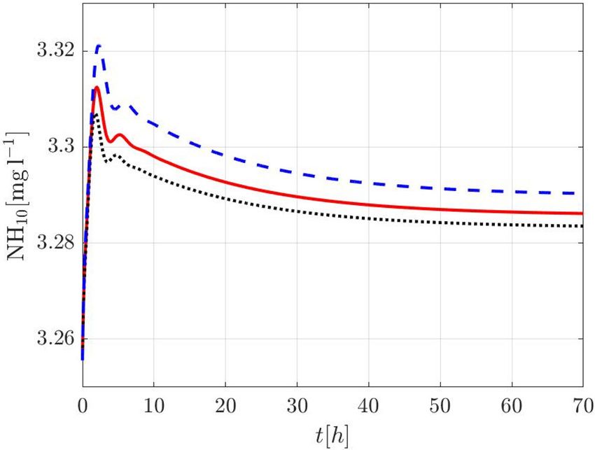
control signals to minimise a multistage cost func- control performance was analysed considering vari-
tion. The GPC method in adaptive and nonadaptive ous criteria.
configuration was applied to a fed-batch penicillin
production in Rodrigues et al. (2002), with the Plant Description
dissolved oxygen concentration as the controlled
variable. The GPC in both, adaptive and nonadap- The carrousel plants represent an important part
tive, configurations improved control performance of the industrial wastewater treatment technology.
of the plant compared to the conventional PID and Overall, these plants usually consist of several con-
predictive Dynamic Matrix Control. In Akay et al. tinuous stirred-tank reactors (CSTR) with a large
(2010), the temperature of a biochemical reactor volume. The disadvantage of this industrial unit is
with baker’s yeast production was controlled using the presence of strong disturbances caused by the
the GPC approach. The control performance was unstable feed flow rate and wastewater composition
analysed considering multiple positive and nega- (Pons, 2011).
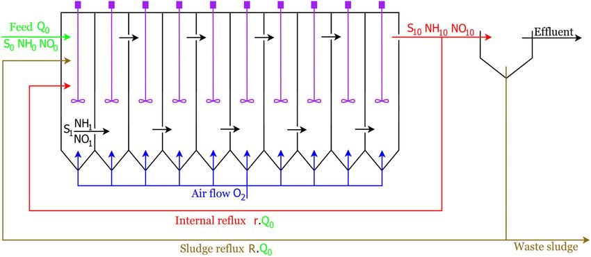
tive step changes of the set point. This research considers a cascade of ten aerated
The behaviour of biochemical reactors, both biochemical reactors for the carrousel activation
continuous and batch, is usually highly nonlinear. shown in Fig. 1 (Derco et al., 1994; Trautenberger,
In some cases, the nonlinearity may cause process- 2017). The given structure of the cascade provides
model mismatch leading to less effective MPC. To both oxic and anoxic environments for the biomass.
overcome this obstacle, robust MPC (RMPC) was Moreover, each bioreactor involves a vertical fan
implemented. There are many forms of RMPC: (aerator) and a supply of airflow, to induce the
e.g., RMPC using linear matrix inequalities (LMIs) required conditions for the biochemical processes
was introduced in Kothrare et al. (1996); Lucia and within the cascade. The feed flow (wastewater)
Engell (2013) designed a nonlinear RMPC for a characterised by the concentration of the organic
batch biochemical reactor and improved its control component (S) and impurities such as ammonium
performance. RMPC formulated using linear ma- salts (NH) or nitrates/nitrites (NO) is fed into the
trix inequalities was designed for a continuously first bioreactor of the cascade. The profile of the
stirred tank reactor (CSTR) in Oravec and Bakošová mixture composition inside the cascade of bioreac-
(2012) and Oravec et al. (2017). tors is the following:
This paper presents the application of various pre- — S0, NH0, NO0 (feed flow),
dictive controllers for a cascade of ten biochemical — S1, NH1, NO1 (output from the first bioreactor),
reactors. The considered plant models wastewater — S10, NH10, NO10 (output from the tenth bioreac-
treatment removing undesired compounds from wa- tor).
ter. Optimal control of these devices is a relevant task A part of a mixture from the tenth bioreactor is
as sustainability is nowadays one of the key require- returned to the first bioreactor as internal reflux
ments of industrial production. This research aims and the rest of the mixture enters the final clarifier.
to compare control performance of conventional The mixture in the final clarifier is separated by the
MPC, GPC and RMPC implemented to the cascade sedimentation process to the effluent and sludge
of ten biochemical reactors using simulations. The flow. The second (sludge) reflux is produced by the
Fig. 1. Flow diagram of the carrousel plant involving the cascade of ten biochemical reactors
and a final clarifier.
52 Mojto M et al., Predictive control of a cascade of biochemical reactors.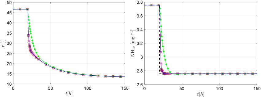
sludge flow from the clarifier and the rest of the                       for the design of MPC and GPC. The robust MPC
sludge leaves the plant as the waste.                                    considered vertex systems are models generated
Mass balance equations of the components of the                          for combinations of minimal and maximal values
mixture were used to design the mathematical                             of uncertain parameters. All obtained vertex sys-
model. These equations follow from the biochemi-                         tems define a convex hull of all possible uncertain
cal processes within the plant, such as carbonisation,                   systems that represent possible behaviour of the
nitrification, and denitrification. Furthermore, the                     cascade of biochemical reactors. The step response
mathematical model includes the Monod equation                           of the process model with nominal, minimal, and
to consider the biomass growth. There are several                        maximal parameters is depicted in Fig. 2.
assumptions of the designed mathematical model,                          To verify the obtained nominal model of the pro-
such as:                                                                 cess, it was compared with the original nonlinear
— feed flow without the suspended or solid particles,
— oxygen does not constrain the processes of car-
   bonisation or nitrification,
— reactors inside the cascade are perfectly mixed
   and variations in the temperature or pH are
   ignored.

Process identification
The purpose of process identification is to gain
desired information about the process dynamics for
further analysis (e.g., design of appropriate control-
lers). The most common structures of the identified
models represent a state-space representation or a
transfer function. In this case, the identified model
represents the transfer function G(s) between:
— the concentration of ammonium salts from the
   tenth bioreactor (NH10, measured variable and                            Fig. 2. Step response of the process model with
   controlled variable in the future),                                      nominal (red solid line), minimal (black dotted
— the ratio of the internal reflux to the feed flow                       line), and maximal (blue dashed line) parameters.
   rate (r, input variable and control input in the
   future),
in the form of Eq. (1). Since a robust approach was
also considered, uncertain parameters were ex-
pressed using interval uncertainty within minimal
and maximal values of each identified parameter.
The resulting transfer function has the following
structure (Furka et al., 2020):
                   b4 s 4 + b3s 3 + b2s 2 + b1s + b0
       G (s ) =                                         ,         (1)
                  a 4 s 4 + a 3s 3 + a 2s 2 + a1s + a 0
The numerator is a polynomial of the fourth order
with the parameters b0—b4 and four zeros. The
denominator structure is the same (fourth order
polynomial with parameters a0—a4) and it involves
four poles. The obtained nominal, minimal and
maximal values of the transfer function parameters                          Fig. 3. Comparison of the step response of the
are stated in Tab. 1. The nominal model with nomi-                           nonlinear process (red dashed line) and the
nal values of identified parameters was considered                            identified nominal model (blue solid line).

Tab. 1. Nominal, maximal, and minimal values of identified model parameters.

   Parameters             b0           b1            b2      b3            b4         a0     a1      a2       a3       a4
    Nominal              0.03         0.83         0.12     0.11        –56.10  –3
                                                                                     0.94   16.77    9.94    5.72     1.00
    Maximal              0.04         1.03         0.13     0.11        –54.10–3     1.29   23.06   12.28    6.39     1.00
    Minimal              0.02         0.65         0.11     0.10        –52.10–3     0.63   11.24    7.74    5.05     1.00

Mojto M et al., Predictive control of a cascade of biochemical reactors.                                                     53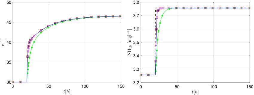
process (Fig. 3). As it can be seen, the discrepancy
ymin £ y (k ) £ y max , (9)
(e.g. sum of squared residuals) between the trajec-
tories is negligible. Therefore, the nominal model Parameter N represents the prediction horizon,
describes the behaviour of the nonlinear plant suf- r(k) Î Rny is the reference, ∆u(k) = u(k) – u(k – 1) is
ficiently. the difference of control action. Variables Q and R
The obtained nominal system can be discretised are tuning matrices weighting control output and
and transformed to the state-space representation. control input. The tuning matrices are positively
This form of the model structure is more accessible definite and diagonal.
for the design of controllers. Considering the pro-
cess dynamics, sampling time Ts = 0.5 h is used for Robust model predictive control
discretisation. The plant-model mismatch is treated in the RMPC
design. The objective of RMPC design is to optimise
Predictive Control Methods the state-feedback control law to compute optimal
control action. Unlike conventional MPC, RMPC
Model predictive control minimises the “worst case” scenario in an infinite cost
The cascade of ten biochemical reactors represents function horizon at each sampling time. The convex
a complex system with disturbances and uncertain- optimisation problem is formulated involving LMIs.
ties. To control this system, linear offset-free MPC In receding horizon setup, RMPC computes the
was designed and to ensure offset-free control of sequence of optimal control actions over the predic-
the plant, augmented model with constant output tion horizon but implements only the first optimal
disturbances was considered (Meader at al., 2009). control action. In order to remove steady-state track-
The augmented state-space model was considered ing error, e(k), the vector of states was extended by an
as follows: integral action in the following way:
x (k +1) = Ax (k ) + Bu (k ), x (0) = x 0 (2) é x (k ) ù
ê ú
x(k ) = êê k ú , e (k ) = r (k ) - y (k ). (13)
y (k ) = Cx (k ) + Fp (k ), (3) ê å e ( j )ú
ú
êë j =0 úû
where k ≥ 0 is a discrete time instant, x(k) Î Rnx re
presents states, u(k) Î Rnu represents control inputs, The extended uncertain state-space model is de-
y(k) Î Rny stands for system outputs and p(k) Î Rnp fined as follows:
stands for constant output disturbances. Parameter (k ) + Bu
(k ), x(0) = x
x(k +1) = Ax 0 (14)
x0 represents the initial conditions of the system.
Furthermore, the discrete state-space representation (k ),
y (k ) = Cx (15)
contains matrices A Î Rnx×nx, B Î Rnx×nu, C Î Rny×nx,
F Î Rny×np representing state, input, output, and dis- where A , B , C are matrices of the system extended
turbance matrices, respectively. subject to integral action.
Based on optimisation, MPC evaluates a sequence of For the purpose of RMPC design, the controlled
optimal control inputs at each sampling time. The plant is represented by an uncertain discrete-time
evaluation considers future behaviour of the model state-space model in the following form:
and constraints of outputs, inputs, and states. After ˆ (k ) + Bu
ˆ (k ), x (0) = x
x(k +1) = Ax 0 (10)
the evaluation of the sequence of optimal control
inputs, MPC considers only the first computed ˆ(k ),
y = Cx (11)
control input to ensure its predictive properties.
The optimisation problem is formulated in the fol-
lowing way: ëê ûú êë ({ ûú )
é Aˆ , Bˆ , Cˆ ù Î convhull é A ( u ) , B ( u ) , C( u ) ù , "u} ,
(12)
N u Î nu
min å (Q r (k ) - y (k ) - R ∆u (k ) ),
2
2
2
2 (4)
∆u ( k )
k =0 where u represents the u-th vertex of the system and
nu represents the total number of system vertices.
s.t. x (k +1) = Ax (k ) + Bu (k ), x (0) = x 0 (5)
Input and output symmetric constraints are formu-
lated as Euclidean and peak norms (Kothrare et al.,
y (k ) = Cx (k ) + Fp (k ), (6)
1996):
u min £ u (k ) £ u max , (7) u (k ) 2£ u sat , u j (k ) £ u sat, j ,
(16)
x min £ x (k ) £ x max , (8) j Î {1, 2, ¼, nu } , y (k ) 2£ ysat ,
54 Mojto M et al., Predictive control of a cascade of biochemical reactors.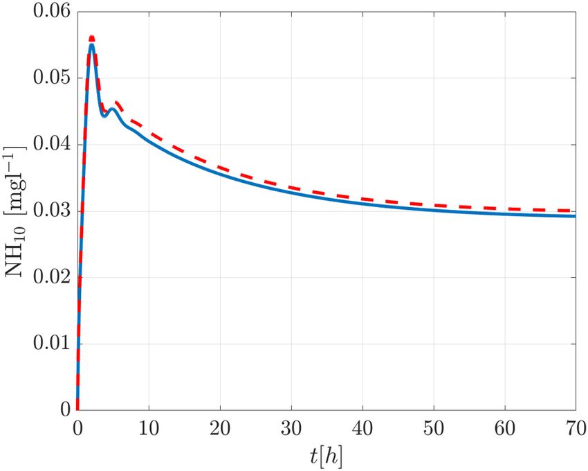
where usat and ysat represent values of the sym-
Xk = gkP–1, P = PT µ 0. (27)
metric constraints on control inputs and outputs,
respectively. However, this approach tends to be Matrix P represents the Lyapunov matrix. The opti-
conservative as it does not operate with the full mised parameter gs,k > 0 shows the weight on uncon-
range of feasible values of control inputs. To over- strained control input. The weighting constant b > 0
come this obstacle, Huang et al. (2011) presented represents another degree of freedom in the MPC
design. Parameters Q Î R x y x y and R Î Rnu ´nu
( n +n )´( n +n )
an improved RMPC design method considering
the presence of actuator saturation and gain are weighting matrices. Matrix Q was extended sub-
matrix of the state-feedback control law was evalu- ject to the extended state vector from Eq. (13).
ated without constraints K (k ) Î R u x y and with
n ´( n +n )
Auxiliary matrix of the controller design without
n ´( n +n )
constraints F (k ) Î R u x y (Huang et al., 2011). constraints, Zk is defined as follows:
The control input in the presence of actuator satu- ,
Zk = KX (28)
ration, us(k) is then computed using the following k
equation matrix Yk represents the auxiliary matrix of
the constrained controller design. parameter
u s (k ) = (Ekm K (k ) + Ekm Fk ) x(k ), (17)
Uk represents auxiliary matrix of inputs of
where parameter Ekm Î Rnu ´ nu , "m Î {1, ¼ 2nu } robust MPC. Symbol * represents the symmetric
is the matrix of all combinations of constrained structure of the matrix, I is the identity matrix of
control inputs. Matrix Ekm Î Rnu ´ nu , "m Î {1, ¼ 2nu } appropriate dimensions and 0 denotes zero matrix
represents the matrix of all combinations of uncon- of appropriate dimensions.
strained control inputs. unconstrained state-feedback controller gain is
then computed as follows:
Ekm = I - Ekm . (18)
K = Zk X k-1 , (29)
The computation of K (k ) and F(k) is transformed
into the following LMIs constrained state-feedback controller gain is then
computed as follows:
min yk + b ys ,k (19)
yk ,X k ,Yk ,U k ,Zk
F = Yk X k-1 . (30)
é Xk * * * ù
ê ú The considered predictive algorithms (RMPC
ê Aˆ X + Bˆ ( u )Y
( u )
Xk * * úú and MPC) require measurements of the states to
ê
ú µ 0,
k k
s.t. ê (20)
ê 1/2
Q Xk 0 gs ,k I * ú compute optimal control input. However, the states
ê ú of the biochemical reactor considered in this paper
êë R1/2Yk 0 0 gs ,k I úû
were not measurable, therefore the Luenberger
é Xk * * * ù state observer was introduced. Detail information
ê ú on the state observer implementation can be found
ê Aˆ ( u )X + Bˆ ( u ) E mZ + E mY * úú
ê k ( k k k k ) Xk * in Furka et al. (2020).
ê ú µ 0, (21)
ê Q X k
1/2
0 gk I * ú
ê ú
ê Generalised predictive control
êë R (Ek Zk + Ek Yk )
1/2 m m
0 0 gk I úú
û The considered cascade of ten bioreactors is a SISO
é 1 *ù system and therefore GPC represents a suitable op-
ê ú µ 0, (22) tion for the control of such a plant. This form of
êx(k ) X k ú
ë û the predictive controller is based on the controlled
éu sat auto-regressive and integrated moving-average
2
I *ù
ê ú µ 0, (23) (CARIMA) model with the following structure:
ê YT X k úû
ë k
d (k )
éU k *ù a(z ) y (k ) = b (z )u (k ) + T (z ) , (31)
D
j , j Î {1, 2, ¼, n u } ,
ê T ú µ 0, U j , j £ u sat,
2
(24)
êYk X k úû
ë where a(z) and b(z) are polynomials representing
é Xk * ù the denominator and numerator of the discrete
ê ú µ 0, (25) transfer function for the process:
êCˆ é Aˆ ( u )X + Bˆ ( u ) E mZ + E mY ù I úú
êë ëê k ( k k k k )ûú 2
ysat
û
a(z ) = 1 + a1z -1 + + an z -n , (32)
g k – gs,k > 0. (26)
b (z ) = b1z -1 + + bm z -m , (33)
Minimisation of auxiliary weight parameter g k > 0
ensures the minimisation of the weighted inverted polynomial T(z) explains the behaviour of the dis-
Lyapunov matrix, Xk, defined as: turbances and d(k) is a random variable with zero
Mojto M et al., Predictive control of a cascade of biochemical reactors. 55mean. The ratio between d(k) and D represents Results and Discussion
slowly varying disturbances.
The advantage of GPC control strategy using the Control setup
CARIMA model is in unbiased prediction provided The offset-free reference tracking problem was
by incorporated estimation of disturbances as the analysed considering a sequence of the step changes
previous equation can be transformed to the follow- of the reference value. The closed-loop control was
ing incremental form: designed in the MATLAB/Simulink R2019a envi-
ronment using CPU i7 3.4 GHz and 8 GB RAM.
a(z )D y (k ) = b (z )Du (k ) + T (z )d (k ), (34)
To formulate optimisation problems of MPC,
where Du(k) = u(k) – u(k – 1). YALMIP (Löfberg 2004), toolbox was introduced.
Subsequently, products in the previous equation The optimisation problem of MPC was solved by
can be modified as follows (Chen, 2013): the GUROBI Optimization (2020). Weighting
matrices Q and R and prediction horizon N were
å
n
i =1
ai D y (k +1- i ) = tuned as:
(35)
= å i =1 bi Du (k - i ) + å i =1Ti d (k - i ).
n n
é0.01 0 0 0 ù
ê ú
Prediction of the output can be derived from the ê 0 0.01 0 0 ú
Q = êê ú , R = 1, N = 30. (43)
left side of Eq. (35): ê 0 0 0.01 0 úú
ê 0 0 0 0.01úúû
n +1 êë
y (k ) + å i =1 (ai - ai -1 )y (k - i ) =
(36)
= å i =1 bi Du (k - i ) + å i =1Ti d (k - i ),
n n The constraints on control input were set as follows:
0 ≤ u(k) ≤ 60. Neither the control output, nor the
where an+1 = 0. states were constrained during the MPC design.
This control strategy determines control input To formulate robust MPC, MUP toolbox was
minimising the following cost function: considered. Semidefinite programming problems
T (SDPs) were formulated using YALMIP (Löfberg,
J = [r (k ) - yˆ(k )] Q [r (k ) - yˆ(k )] + Du (k )T R Du (k ), (37)
2004) and solved by MOSEK (MOSEK ApS., 2019).
where yˆ(k ) = G Du (k ) + yˆ* (k ), variables Q and R are Variables Q and R were systematically tuned as
tuning matrices and G is a lower-triangular matrix follows:
(Clarke et al., 1987).
é0.01 0 0 0 0ù
The output prediction assuming Du(k) = 0 is ex- ê ú
ê 0 0.01 0 0 0ú
pressed by: ê ú
Q = êê 0 0 0.01 0 0úú , R = 1. (44)
y * (k + j ) = H F j x(k ) + H F j -1L[ y (k ) - Hx(k )], (38) ê 0
ê 0 0 0.01 0úú
where the structure of matrices HFj and HFj–1 is ê 0 0 0 0 5úúû
ëê
shown in (Chen, 2013).
The following structure of input increment can be The constraints on control input were set as fol-
derived by setting the gradient of Eq. (37) to zero lows: 0 ≤ u(k) ≤ 60. The control output was not
(Grimble, 1992): constrained during the design of robust MPC.
When designing MPC and RMPC, the Luenberger
Du (k ) = (G T QG + R )-1G T Q éër (k ) - y * (k )ùû = state observer was considered to augment the state-
39)
= K éër (k ) - y * (k )ùû , space from Eq. (2). The disturbance matrix was
considered as follows:
where K is the gain of the controller.
F = 1. (45)
The state-space representation is derived using
observable canonical form realisation. The model The state-observer used observer gain designed
structure has the following form: using pole placement in the following way:
x(k + 1) = Fx(k) + GDu(k) + Ld(k), (40) é 0.047 ù
ê ú
ê 1.935 ú
y(k) = Hx(k) + d(k), (41) ê ú
L = êê-70.218úú . 46)
matrices F, G, L and H are defined in (Chen, 2013). ê 300.593 ú
ê ú
The suitable state observer for the designed state- ê 6.593 ú
ëê ûú
space model (Eq. (40)) is written as:
The setup of prediction horizon N and weighting
x(k +1) = Fx(k ) + GDu (k ) + L[ y (k ) - Hx(k )]. (42)
matrices (Q and R) of the GPC control strategy is
56 Mojto M et al., Predictive control of a cascade of biochemical reactors.the same as in case of MPC (see Eq. (43)). Due to ensure the consistency of the results, similar values
relatively long prediction horizon, it is impractical of weighting matrices were considered in all predic-
to display matrix G Î RN×N (see Eq. (39)) from the tive methods. The performance of designed control
structure of the GPC controller. As it was mentioned strategies was also compared by integral absolute
before, matrices of the state-space observer (F, G, L error (IAE) and integral squared error (ISE). These
and H) were designed according to Chen (2013). criteria have the following structures:
IAE = å k =0 e (k ) , IAE = å k =0 e (k )2 ,
150 150
Control performance (47)
The designed predictive controllers were considered
to control the plant described by the linear transfer where e(k) is the control error. The resulting values
function in Eq. (1). To compare the controllers, two of IAE and ISE criteria are listed in Tab. 2. The ob-
reference step changes were generated, one positive tained values confirm better control performance
and one negative. The controlled output is depicted of MPC, and GPC compared to RMPC.
in Fig. 4a) and Fig 5a). The corresponding control The resulting trajectories show that all the designed
input is depicted in Fig. 4b) and Fig 5b). All predic- controllers removed the steady-state control error,
tive controllers were compared by simulation using and each controlled system reached the reference
the nominal model of the biochemical reactor. To value without offset. Moreover, MPC and RMPC
a) Control input to the process b) Output from the process
Fig. 4. Comparison of the control performance provided by positive reference step change. MPC (□),
RMPC (●), GPC (*), reference (dashed black) line.
a) Control input to the process b) Output from the process
Fig. 5. Comparison of the control performance provided by negative reference step change. MPC (□),
RMPC (●), GPC (*), reference (dashed black) line.
Mojto M et al., Predictive control of a cascade of biochemical reactors. 57Tab. 2. Comparison of IAE [mg l–1 h] and ISE [mg2 l–2 h] criteria of the designed controllers.
Criterion IAE [mg l–1 h] ISE [mg2 l–2 h]
Controller MPC RMPC GPC MPC RMPC GPC
First step change 1.5580 4.7197 1.5594 0.5176 1.2543 0.5205
Second step change 3.1161 9.9396 3.1189 2.0704 5.6376 2.0820
Sum 4.6741 14.6593 4.6783 2.5880 6.8919 2.6025
satisfied the constraints on the control input. The performance of the designed controllers was
GPC did not consider constraints on the control compared using integral criteria. As expected, the
input during the design. conventional MPC and GPC control performance
According to the results, MPC and GPC achieved was almost identical. Application of the RMPC
almost the same control performance. This is decreased the control performance; however, this
mainly caused by the assumption that the controlled approach is able to handle uncertain and non
process is a single-input-single-output system. linear behaviour of the plant.
Variations of the feed flow rate represent external
disturbance. In the simulation results, variations of Acknowledgement
the feed flow were considered to be minor and oc- The authors gratefully acknowledge the con-
casional and compensated by a well-tuned controller. tribution of the Scientific Grant Agency of the
If the disturbance is significant, it could be measured Slovak Republic under the grants 1/0585/19 and
to design a control loop with disturbance rejection. 1/0545/20, the Slovak Research and Development
Moreover, significant variations of the feed flow rate Agency under the project APVV-15-0007. M. Hor-
can still be reduced by storing the feed in additional váthová was also supported by an internal STU
tank before it enters the carrousel plant. grant.
The output variable of the process (Fig. 4b and 5b)
was stabilized faster than the input variable (Fig. 4a References
and 5a). The reason is the presence of a stable zero
in the transfer function of the studied process. All Akay B, Ertunç S, Bursali N, Hapoğlu H, Alpbaz M
designed controllers try to compensate the effect (2010) Application of generalized predictive control
to baker’s yeast production, Chemical Engineering
of this zero and therefore the input variable is
Communications, 190: 999—1017.
still varying while the output variable is already in Chang L, Xinggao L, Henson MA (2016) Nonlinear
steady state. model predictive control of fed-batch fermentations
There are also slight differences between the input using dynamic flux balance models, Journal of Process
trajectory of RMPC and of other controllers. This Control, 42: 137—149.
is reflected in the increased settling time and both Chen Y (2013) A Novel DMC-Like Implementation of
IAE and ISE criteria. This is an expected result be- GPC, 2013 International Conference on Mechatronic
Sciences, Shenyang, China: 362—366.
cause unlike other controllers, the design of RMPC
Clarke DW, Mohtadi C, Tuffs PS (1987) Generalized
includes an uncertain model of the plant. If the predictive control — Part I. The basic algorithm,
case study considered control of a nonlinear model, Automatica, 23: 137—148.
RMPC would be expected to outperform both MPC Craven S, Whelan J, Glennon B (2014) Glucose
and GPC, as the process model mismatch would be concentration control of a fed-batch mammalian
significant. cell bioprocess using a nonlinear model predictive
controller, Journal of Process Control, 24: 344—357.
Derco J, Hutňan M, Králik M (1994) Modelling
Conclusion of carrousel type activation (in Slovak), Vodní
hospodářství, 42: 23—27.
In this paper, the design and application of Furka M, Kiš K, Horváthová M, Mojto M, Bakošová
multiple predictive controllers were investigated. M, (2020) Identification and Control of a Cascade
The controllers were applied for a cascade of ten of Biochemical Reactors, 2020, Cybernetics &
biochemical reactors using simulations. First, Informatics, Velké Karlovice, Czech Republic.
conventional MPC and GPC were designed for a Grimble MJ (1992) Generalized predictive optimal
control: An introduction to the advantages and
nominal model of the plant. RMPC was designed,
limitations, International Journal of System Science
considering an uncertain model of the plant. To 23: 85—98.
design the RMPC, LMI-based approach with re- GUROBI Optimization (2020) GUROBI Optimizer
duced conservativeness was applied. The control Quick Start Guide. Version 9.0.
58 Mojto M et al., Predictive control of a cascade of biochemical reactors.Henson MA (2006) Biochemical reactor modeling and Pons MN, Mourot G, Ragot J (2011) Modeling and control, IEEE Control Systems Magazine, 26: 54—62. simulation of a carrousel for long-term operation, Huang H, Li D, Lin Z, Xi Y (2011) An improved robust IFAC World Congress, Milan, Italy. model predictive control design in the presence of Rajinikanth V, Latha K (2010) Identification and Control actuator saturation, Automatica, 47: 861—864. of Unstable Biochemical Reactor, International Kothare MV, Balakrishnan V, Morari M (1996) Robust Journal of Chemical Engineering and Applications, 1: constrained model predictive control using linear 106—111. matrix inequalities, Automatica, 32: 1361—1379. Ramaswamya S, Cutrightb TJ, Qammar HK (2005) Löfberg J (2004) YALMIP: A Toolbox for Modeling Control of a continuous bioreactor using model and Optimization in MATLAB, Proceedings. of the predictive control, Process Biochemistry, 40: CACSD Conference, Taipei, Taiwan. 2763—2770. Lucia S, Engell S (2013) Robust nonlinear model Rodrigues JAD, Toledo ECV, Maciel Filho R (2002) predictive control of a batch bioreactor using multi- A tuned approach of the predictive–adaptive GPC stage stochastic programming, European Control controller applied to a fed-batch bioreactor using ConfeSCHrence (ECC), Zurich, Switzerland. complete factorial design, Computers & Chemical MOSEK ApS. (2019) The MOSEK optimization toolbox Engineering, 26: 1493—1500. for MATLAB manual. Version 9.0. Vinopraba T, Sivakumaran N, Narayanan S, Oravec J, Bakošová M (2012) Robust Constrained MPC Radhakrishnan TK (2013) Design of fractional order Stabilization of a CSTR, Acta Chimica Slovaca, 5: controller for Biochemical reactor, IFAC Proceedings 153—158. Volumes, 46: 205—208. Oravec J, Bakošová M (2015) Software for efficient Smets IY, Claes JE, November EJ, Georges BP, Van Impe LMI-based robust MPC design, Proceedings of the JF (2004) Optimal adaptive control of (bio)chemical 20th International Conference on Process Control, reactors: past present and future, Journal of Process Štrbské Pleso, Slovakia, 272—277. Control, 14: 795—805. Oravec J, Bakošová M, Hanulová L, Horváthová M Trautenberger R (2017) Modelling and control of a (2017) Design of Robust MPC with Integral Action cascade of biochemical reactors, Bachelor Thesis, for a Laboratory Continuous Stirred-Tank Reactor, SCHK, Bratislava, Slovakia. Proceedings of the 21st International Conference on Process Control, Štrbské Pleso, Slovakia, 459—464. Mojto M et al., Predictive control of a cascade of biochemical reactors. 59
You can also read