Turpike Control and Machine Learning - Enrique Zuazua
←
→
Page content transcription
If your browser does not render page correctly, please read the page content below

Turpike Control and Machine Learning

                                                      Enrique Zuazua

                                       Chair of Dynamics, Control and Numeric
                                                      FAU - Erlangen - Germany
                                                Department       of Data Scienc
                                                       enrique.zuazua@fau.de
                                                                FA
                                                 https://www.caa-avh.nat.fau.eu
                   Based on joint work with Borjan Geshkovski, Carlos Esteve, Dario Pighin and Domenec Ruiz-Balet
                                                       Erlangen, German
                                                   https://caa-avh.nat.fau.eu
                                      Paris Bachelier Seminar, 21.05.2021

     E. Zuazua (FAU - AvH)                              Turpike-Control-ML                                  Bachelier, 21.05.2021   1 / 41
U

            y

                       e

                                         s
Control

    Outline

1    Control

2    Turnpike

3    Deep learning

        E. Zuazua (FAU - AvH)   Turpike-Control-ML   Bachelier, 21.05.2021   2 / 41
Control

 Historical perspective: Cybernetics

“Cybernétique” was proposed by the French physicist A.-M. Ampère in the XIX Century to
design the nonexistent science of process controlling. This was quickly forgotten until 1948, when
Norbert Wiener (1894–1964) chose “Cybernetics” as the title of his famous book.
Wiener defined Cybernetics as “ the science of control and communication in animals and
machines”.1
In this way, he established the connection between Control Theory and Physiology and
anticipated that, in a desirable future, engines would obey and imitate human beings.

  1
      “What we want is a machine that can learn from experience.“ Alan Turing, 1947.
          E. Zuazua (FAU - AvH)                        Turpike-Control-ML              Bachelier, 21.05.2021   3 / 41
Control

 Controllability

Let n, m 2 N⇤ and T > 0 and consider the following linear finite-dimensional system

                               x 0 (t) = Ax(t) + Bu(t),      t 2 (0, T );         x(0) = x 0 .                           (1)

In (1), A is a n ⇥ n real matrix, B is of dimensions n ⇥ m and x 0 is the initial sate of the sytem in
Rn . The function x : [0, T ] ! Rn represents the state and u : [0, T ] ! Rm the control.
¿Can we control the state x of n components with only m controls, even if n >> m so that, for
instance x(T ) = 0?

Theorem

(1958, Rudolf Emil Kálmán (1930 – 2016 )) System (1) is controllable i↵

                                         rank [B, AB, · · · , An        1
                                                                            B] = n.

       E. Zuazua (FAU - AvH)                       Turpike-Control-ML                            Bachelier, 21.05.2021   4 / 41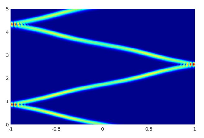
Control

 Sketch of the proof
From the variation of constants formula:
                             Z t                               Z         t   X (t     s)k k
           x(t) = e At x 0 +     e A(t s) Bu(s)ds = e At x 0 +                           A Bu(s)ds.
                                      0                                  0 k   0
                                                                                    k!

By Cayley2 -Hamilton’s         3   theorem Ak , for k    n, is a linear combination of I , A, ..., An    1.

The Kalman rank condition assures that, manipulating the last term due to the variation of
constants formula, out of a strategic choice of the control u(t), the solution can be driven to any
destination x(T ).

  2
    Arthur Cayley (UK, 1821 - 1895)
  3
    William Rowan Hamilton (Ireland, 1805 - 1865)
       E. Zuazua (FAU - AvH)                        Turpike-Control-ML                     Bachelier, 21.05.2021   5 / 41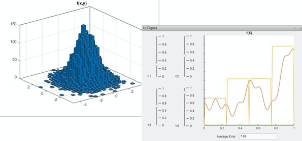
Control

 An example: Nelson’s car.

                Two controls suffice to control a four-dimensional dynamical system.

E. Sontag, Mathematical control theory, 2nd ed.,Texts in Applied Mathematics,vol.6,
Springer-Verlag, NewYork,1998.

      E. Zuazua (FAU - AvH)                Turpike-Control-ML                Bachelier, 21.05.2021   6 / 41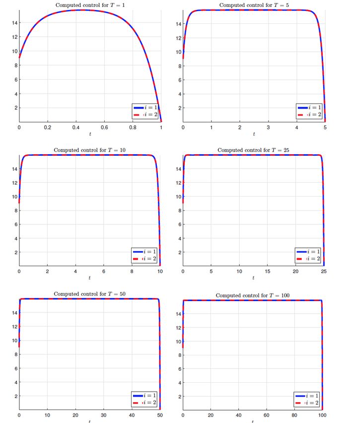
Control
Duality, J.-L. Lions, SIREV, 1988
Consider the adjoint system ⇢
p 0 = A⇤ p, t 2 (0, T )
(2)
p(T ) = pT
and minimize Z
1 T
J(pT ) = | B ⇤ p |2 dt + hx 0 , p(0)i
2 0
Then
u = B ⇤ pb
is the control of minimal L2 -norm.4
And the functional J is coercive i↵ the Kalman rank condition is satisfied.
The Kalman condition is equivalent to the Unique Continuation property
B ⇤ p ⌘ 0 ) p T ⌘ 0.
The observability inequality plays a key role
Z T
||p T ||2 C | B ⇤ ' |2 dt
0
4
This confirms Wiener’s vision ”..control and communication...”
E. Zuazua (FAU - AvH) Turpike-Control-ML Bachelier, 21.05.2021 7 / 41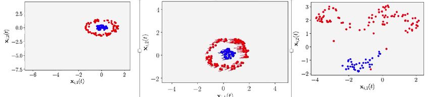
Turnpike

    Outline

1    Control

2    Turnpike

3    Deep learning

        E. Zuazua (FAU - AvH)   Turpike-Control-ML   Bachelier, 21.05.2021   8 / 41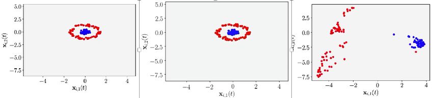
Turnpike

 Sonic boom
 Francisco Palacios, Boeing, Long Beach, California, Project Manager and Aerodynamics Engineer

     Goal: the development of supersonic aircrafts, sufficiently quiet to be allowed to fly
     supersonically over land.
     The pressure signature created by the aircraft must be such that, when reaching ground, (a)
     it can barely be perceived by humans, and (b) it results in admissible disturbances to
     man-made structures.
     This leads to an inverse design or control problem in long time horizons.

   Juan J. Alonso and Michael R. Colonno, Multidisciplinary Optimization with Applications to
            Sonic-Boom Minimization, Annu. Rev. Fluid Mech. 2012, 44:505 – 526.

Many other challenging problems of high societal impact raise similar issues: climate change,
sustainable growth, chronically deseases, design of long lasting devices and infrastructures...

        E. Zuazua (FAU - AvH)                        Turpike-Control-ML                          Bachelier, 21.05.2021   9 / 41
Turnpike
Origins
Although the idea goes back to John von Neumann in 1945, Lionel W. McKenzie traces the term
to Robert Dorfman, Paul Samuelson, and Robert Solow’s ”Linear Programming and Economics
Analysis” in 1958, referring to an American English word for a Highway:5
6
... There is a fastest route between any two points; and if the origin and destination are
close together and far from the turnpike, the best route may not touch the turnpike.
But if the origin and destination are far enough apart, it will always pay to get on to the
turnpike and cover distance at the best rate of travel, even if this means adding a little
mileage at either end.
5
A. J. Zaslavski, Springer, New York, 2006.
6
L. Grüne, Automatica, 49, 725-734, 2013
E. Zuazua (FAU - AvH) Turpike-Control-ML Bachelier, 21.05.2021 10 / 41Turnpike
Substantiation and preliminary conclusion
We implement turnpike (or nearby) strategies most often. And it is indeed a good idea to do it!
But this requires that the system under consideration to be controllable/stabilisable.
E. Zuazua (FAU - AvH) Turpike-Control-ML Bachelier, 21.05.2021 11 / 41Turnpike Control The PDE-Turnpike Paradox
Wave propagation: Why do not we see the turnpike?
Typical controls for the wave equation exhibit an oscillatory behaviour, and this
independently of the length of the control time-horizon.
This fact is intrinsically linked to the oscillatory nature of wave propagation.
Waves are controlled through anti-waves, reproducing an oscillatory pattern.
E. Zuazua (FAU - AvH) Turnpike Control and Deep Learning MOX-Politecnico-Milano, 10.12.2020 7 / 42Turnpike
Heat and di↵usion processes: Why do not we see the turnpike either?
Typical controls for the heat equation exhibit unexpected oscillatory and concentration e↵ects.
This was observed by R. Glowinski and J. L. Lions in the 80’s in their works in the numerical
analysis of controllability problems for heat and wave equations.
Why? Lazy controls?
E. Zuazua (FAU - AvH) Turpike-Control-ML Bachelier, 21.05.2021 12 / 41Turnpike Control The PDE-Turnpike Paradox
Optimal controls are boundary traces of solutions of the adjoint problem through the optimality
system or the Pontryagin Maximum Principle, and solutions of the adjoint heat equation
pt p=0
look precisely this way.
Large and oscillatory near t = T they decay and get smoother when t gets down to t = 0. And
this is independent of the time control horizon [0, T ].
For wave-like equations ontrols are given by the solutions of the adjoint system
ptt p=0
that exhibit endless oscillations.
First conclusion:
Typical control problems for wave and heat equations do not seem to exhibit the turnpike
property.
These are the controls of L2 -minimal norm. There are many other possibilities for successful
control strategies (sparse controls by L1 -minimisation, bang-bang controls...)
May be the Turnpike Principle does not hold for for Partial Di↵erential Equations (PDE), i. e.
Infinite-Dimensional Dynamical Systems?
E. Zuazua (FAU - AvH) Turnpike Control and Deep Learning MOX-Politecnico-Milano, 10.12.2020 9 / 42Turnpike
The control problem for di↵usion : A closer look
Let n 1 and T > 0, ⌦ be a simply connected, bounded domain of Rn with smooth boundary ,
Q = (0, T ) ⇥ ⌦ and ⌃ = (0, T ) ⇥ :
8
< yt y = f 1! in Q
y =0 on ⌃ (3)
:
y (x, 0) = y 0 (x) in ⌦.
1! = the characteristic function of ! of ⌦ where the control is active.
We know that y 0 2 L2 (⌦) and f 2 L2 (Q) so that (3) admits a unique solution
y 2 C [0, T ] ; L2 (⌦) \ L2 0, T ; H01 (⌦) .
y = y (x, t) = solution = state, f = f (x, t) = control
Goal: Drive the dynamics to equilibrium by means of a suitable choice of the control
y (·, T ) ⌘ y ⇤ (x).
E. Zuazua (FAU - AvH) Turpike-Control-ML Bachelier, 21.05.2021 13 / 41Turnpike
We address this problem fro a classical optimal control / least square approach:
Z T Z Z
1
min |f |2 dxdt + |y (x, T ) y ⇤ (x)|2 dx .
2 0 ! ⌦
According to Pontryagin’s Maximum Principle the Optimality System (OS) reads
yt y = p1! in Q
pt p = 0 in Q
y = 0 on ⌃
y (x, 0) = y 0 (x) in ⌦
p(x, T ) = y (x, T ) y ⇤ (x) in ⌦
p = 0 on ⌃.
And the optimal control is:
f (x, t) = p(x, t) in ! ⇥ (0, T ).
E. Zuazua (FAU - AvH) Turpike-Control-ML Bachelier, 21.05.2021 14 / 41Turnpike Control Linear PDE revisited
By duality (Fenchel-Rockafellar) the adjoint p at time t = T , p T saturates the regularity
properties required to assure the well-posedness of the functional:
H = {p T : p(x, 0) 2 L2 (⌦)}
This is a huge space, allowing an exponential increase of Fourier coefficients at high frequencies.
And, because of this, we observe the tendency of the control to concentrate all the action in the
final time instant t = T , incompatible with turnpike e↵ects4
10
x 10
4
3
2
1
0
!1
!2
!3
0 0.1 0.2 0.3 0.4 0.5 0.6 0.7 0.8 0.9 1
x
Tychono↵’s monster (1935)
4
A. Münch & E. Z., Inverse Problems, 2010
E. Zuazua (FAU - AvH) Turnpike Control and Deep Learning MOX-Politecnico-Milano, 10.12.2020 12 / 42Turnpike
Remedy: Better balanced controls
Let us now consider the control f minimising a compromise between the norm of the state and
the control among the class of admissible controls:
Z T Z Z TZ Z
1
min |y |2 dxdt + |f |2 dxdt + |y (x, T ) y ⇤ (x)|2 .
2 0 ⌦ 0 ! ⌦
Then the Optimality System reads
yt y = p1! in Q
pt p = y in Q
y = p = 0 on ⌃
y (x, 0) = y 0 (x) in ⌦
p(x, T ) = y (x, T ) y ⇤ (x) in ⌦
We now observe a coupling between p and y on the adjoint state equation!7
y y
x x
7
A. Porretta & E. Z., SIAM J. Cont. Optim., 2013.
E. Zuazua (FAU - AvH) Turpike-Control-ML Bachelier, 21.05.2021 15 / 41Turnpike Control Linear PDE revisited
New Optimality System Dynamics
What is the dynamic behaviour of solutions of the new fully coupled OS?
For the sake of simplicity, assume ! = ⌦.
The dynamical system now reads
yt y = p
pt + p= y
This is a forward-backward parabolic system.
A spectral decomposition exhibits the characteristic values
q
µ±
j = ± 1 + 2
j
where ( j )j 1 are the (positive) eigenvalues of .
Thus, the system is the superposition of growing + diminishing real exponentials.
y y
x x
E. Zuazua (FAU - AvH) Turnpike Control and Deep Learning MOX-Politecnico-Milano, 10.12.2020 14 / 42Turnpike Control Linear PDE revisited
The turnpike property for the heat equation
New dynamics = combination of exponentially stable and unstable branches ⌘ compatible with turnpike
The turnpike behaviour is ensured when T ! 1 when the cost functional penalizes sufficiently
state and control.
[Controllability] + [Coercive in state + control cost] ! Turnpike
The same occurs for wave propagation5
5
M. Gugat, E. Trélat, E. Zuazua, Systems and Control Letters, 90 (2016), 61-70.
E. Zuazua (FAU - AvH) Turnpike Control and Deep Learning MOX-Politecnico-Milano, 10.12.2020 15 / 42Turnpike Control General theory
Linear theory. Joint work with A. Porretta, SIAM J. Cont. Optim., 2013.
The same methods apply in the inifinite-dimensional context, covering in particular linear heat
and wave equations
Consider the finite dimensional dynamics
(
xt + Ax = Bu
(2)
x(0) = x0 2 RN
where A 2 M(N, N), B 2 M(N, M), with control u 2 L2 (0, T ; RM ).
Given a matrix C 2 M(N, N), and some x ⇤ 2 RN , consider the optimal control problem
Z T
1
T
min J (u) = (|u(t)|2 + |C (x(t) x ⇤ )|2 )dt .
u 2 0
There exists a unique optimal control u(t) in L2 (0, T ; RM ), characterized by the optimality
condition
( (
x + Ax = BB ⇤ p p + A ⇤ p = C ⇤ C (x x ⇤)
t t
u = B⇤p , , (3)
x(0) = x0 p(T ) = 0
E. Zuazua (FAU - AvH) Turnpike Control and Deep Learning MOX-Politecnico-Milano, 10.12.2020 16 / 42Turnpike Control General theory
The steady state control problem
The same problem can be formulated for the steady-state model
Ax = Bu.
Then there exists a unique minimum ū, and a unique optimal state x̄, of the stationary control
problem
1
min Js (u) = (|u|2 + |C (x x ⇤ )|2 ) (4)
u 2
which is nothing but a constrained minimization in RN .
The optimal control ū and state x̄ satisfy
ū = B ⇤ p̄ , Ax̄ = B ū , and A⇤ p̄ = C ⇤ C (x̄ x ⇤) .
E. Zuazua (FAU - AvH) Turnpike Control and Deep Learning MOX-Politecnico-Milano, 10.12.2020 17 / 42Turnpike Control General theory
We assume that
(A, B) is controllable, (5)
or, equivalently, that the matrices A, B satisfy the Kalman rank condition
h i
Rank B AB A2 B . . . AN 1 B = N . (6)
Concerning the cost functional, we assume that the matrix C is such that (void assumption when
C = Id)
(A, C ) is observable (7)
which means that the following algebraic condition holds:
h i
Rank C CA CA2 . . . CAN 1 = N . (8)
xt + Ax = Bu
Z T
1
J T (u) = (|u(t)|2 + |C (x(t) x ⇤ )|2 )dt
2 0
(
xt + Ax = Bu
pt + A⇤ p = C ⇤ Cx
E. Zuazua (FAU - AvH) Turnpike Control and Deep Learning MOX-Politecnico-Milano, 10.12.2020 18 / 42Turnpike Control General theory
Proofs
Proof # 1: Dissipativity
d ⇥ ⇤ 2 2
⇤
[(x x̄)(p p̄)] = B (p p̄)| + |C (x x̄)|
dt
That is the starting point of a turnpike proof. Note however that it is much trickier than the
classical Lyapunov stability: Two boundary layers at t = 0 and t = T , moving time-horizon
[0, T ]...
Proof #2 : Riccati
Consider the Infinite Horizon Linear Quadratic Regulator (LQR) problem in [0, 1) with null
target x ⇤ ⌘ 0.
Employ Riccati feedback exponential stabilizator.
Cut-it-o↵ onto [0, T ].
Correct the boundary layer at t = T to match the terminal conditions .
Proof # 3: Singular perturbations Implement the change of variables t ! sT :
t 2 [0, T ] () s 2 [0, 1].
System
xt + Ax = Bu, t 2 [0, T ]
becomes
1
xs + Ax = Bu, s 2 [0, 1]
T
As T ! 1, " = 1/T ! 0.
E. Zuazua (FAU - AvH) Turnpike Control and Deep Learning MOX-Politecnico-Milano, 10.12.2020 20 / 42Turnpike Control Perspectives
Nonlinear problems
A. Porretta & E. Z., Mathematical Paradigms of Climate Science, Springer INdAM Series, 2016.
The theory can be extended for semilinear PDEs provided the target is small employing
linearization techniques.
But numerical simulations shows that the property is much more robust. 6
Developing a complete theorem, for large targets and deformations, is a challenging problem.
6
Simulations by S. Volkwein for a cubic semilinear equation with large targets.
E. Zuazua (FAU - AvH) Turnpike Control and Deep Learning MOX-Politecnico-Milano, 10.12.2020 21 / 42Turnpike Control Perspectives
Heuristic explanation and practical use
In applications and daily life we use a quasi-turnpike principle, which is very robust and
ubiquitous, even in the context of multiple steady optima (local or global):
Step 1: Compute the optimal steady optimal control and state,
Step 2: Drive the system from the initial configuration to this steady state one;
Step 3: Remain in this steady configuration as long as possible;
Step 4: Exit this configuration if a terminal condition is to be met.
E. Zuazua (FAU - AvH) Turnpike Control and Deep Learning MOX-Politecnico-Milano, 10.12.2020 22 / 42Turnpike Control Perspectives
Warning! Long time numerics plays a key role: Geometric/Symplectic
integration; Well balanced numerical schemes...
Numerical integration of the pendulum (A. Marica)
E. Zuazua (FAU - AvH) Turnpike Control and Deep Learning MOX-Politecnico-Milano, 10.12.2020 23 / 42Turnpike Control Perspectives
An open problem and biblio
Further extend the turnpike theory for nonlinear PDE, getting rid of the smallness condition on
the target, which in numerical simulations seems to be unnecessary.
A. Porretta, E. Z., SIAM J. Control. Optim., 51 (6) (2013), 4242-4273.
A. Porretta, E. Z., Springer INdAM Series ”Mathematical Paradigms of Climate Science”, F.
Ancona et al. eds, 15, 2016, 67-89.
E. Trélat, E. Z., JDE, 218 (2015) , 81-114.
M. Gugat, E. Trélat, E. Z., Systems and Control Letters, 90 (2016), 61-70.
E. Z., Annual Reviews in Control, 44 (2017) 199-210.
E.Trélat, C. Zhang, E. Z., SIAM J. Control Optim. 56 (2018), no. 2, 1222–1252.
V. Hernández-Santamaria, M. Lazar, E.Z. Numerische Mathematik (2019) 141:455-493.
D. Pighin, N. Sakamoto, E. Z., IEEE CDC Proceedings, Nice, 2019.
G. Lance, E. Trélat, E. Z., Systems & Control Letters 142 (2020) 104733.
J. Heiland, E. Z., arXiv:2007.13621, 2020.
C. Esteve, H. Kouhkouh, D. Pighin, E. Z., arxiv.org/pdf/2006.10430, 2020.
M. Gugat, M. Schuster and E. Z., SEMA/SIMAI Springer Series, 2020.
And further interesting work by collaborators: S. Zamorano (NS), M. Warma & S. Zamorano,
Fractional heat,...
Our thanks to our FAU colleague Daniel Tenbrinck. He suggested to us to explore turnpike for
Neural Networks.
E. Zuazua (FAU - AvH) Turnpike Control and Deep Learning MOX-Politecnico-Milano, 10.12.2020 24 / 42Deep learning
Outline
1 Control
2 Turnpike
3 Deep learning
E. Zuazua (FAU - AvH) Turpike-Control-ML Bachelier, 21.05.2021 16 / 41Deep learning
Universal approximation theorem I
E. Zuazua (FAU - AvH) Turpike-Control-ML Bachelier, 21.05.2021 17 / 41Deep learning
Universal approximation theorem II
Hyperbolic tangent Rectified Linear Unit (ReLU)
1 5
0.8 4.5
0.6 4
0.4 3.5
0.2 3
0 2.5
y
y
-0.2 2
-0.4 1.5
-0.6 1
-0.8 0.5
-1 0
-5 -4 -3 -2 -1 0 1 2 3 4 5 -5 -4 -3 -2 -1 0 1 2 3 4 5
x x
E. Zuazua (FAU - AvH) Turpike-Control-ML Bachelier, 21.05.2021 18 / 41Deep learning
Supervised learning
Goal: Find an approximation of a function f⇢ : Rd ! Rm from a dataset
N
~
xi , ~
yi i=1
⇢ Rd⇥N ⇥ Rm⇥N
drawn from an unknown probability measure ⇢ on Rd ⇥ Rm .
Classification: match points (images) to respective labels (cat, dog).
! Popular method: training a neural network.
E. Zuazua (FAU - AvH) Turpike-Control-ML Bachelier, 21.05.2021 19 / 41Deep learning
Residual neural networks
[1] K He, X Zhang, S Ren, J Sun, 2016: Deep residual learning for image recognition
[2] E. Weinan, 2017. A proposal on machine learning via dynamical systems.
[3] R. Chen, Y. Rubanova, J. Bettencourt, D. Duvenaud, 2018. Neural ordinary di↵erential equations.
[4] E. Sontag, H. Sussmann, 1997, Complete controllability of continuous-time recurrent neural networks.
ResNets
(
xk+1
i = xk
i + hW k
(A k k
xi + b k
), k 2 {0, . . . , Nlayers 1}
x0i = x̃i , i = 1, ..., N
where h = 1, globally Lipschitz (0) = 0.
nODE
T
Layer = timestep; h = Nlayers
for given T > 0
(
ẋi (t) = W (t) (A(t)xi (t) + b(t)) for t 2 (0, T )
xi (0) = ~xi , i = 1, ..., N
The problem becomes then a giant simultaneous control problem in which each initial datum xi (0)
needs to the driven to the corresponding destination for all i = 1, ..., N with the same controls:
What happens when T ! 1, i.e. in the deep, high number of layers regime?8 9
8
C. Esteve, B. Geshkovski, D. Pighin, E. Zuazua, Large-time asymptotics in deep learning, arXiv:2008.02491
9
D. Ruiz-Balet & Zuazua, Neural ODE control for classification, approximation and transport, arXiv:2104.05278
E. Zuazua (FAU - AvH) Turpike-Control-ML Bachelier, 21.05.2021 20 / 41Deep learning
Special features of the control of ResNets
Nonlinearities are unusual in Mechanics: is flat in half of the phase space.
We need to control many trajectories (one per item to be classified) with the same control!
10
The very nature of the activation function allows actually to achieve this monster simultaneous
control goal. The fact that leaves half of the phase space invariant while deforming the other
one, allows to build dynamics that are not encountered in the classical ODE systems in mechanics
and for which such kind of simultaneous control property is unlikely or even impossible.
10
This would be impossible for instance, for the standard linear system x 0 = Ax + Bu.
E. Zuazua (FAU - AvH) Turpike-Control-ML Bachelier, 21.05.2021 21 / 41Deep learning
Turnpike for ResNets
T !1 ⇠ Nlayers ! 1.
Turnpike refers to the fact that, in long time-horizons, optimal controls and trajectories are
exponentially close to the optimal steady-state control and state in most of the time-horizon.
Supervised Learning* () minimize11
Z T
1
kPx(t) y k2 dt + ↵ kuk2H 1 (0,T ;Rdu ). (SL*)
N 0
yN ], u := [A, W , b] in (20) and P : Rd ! Rm .
y1 , . . . , ~
y := [~
Theorem (Turnpike): Under controllability assumptions, for any sufficiently large T ,
an optimal solution (uT , xT ) to (SL*)–(20) satisfies
kuT kH 1 (0,T ;Rdu ) C1
and
µt
kPxT (t) y k C2 e 8t 2 [0, T ]
for some C1 > 0, C2 > 0 and µ > 0, all independent of T .
11
Note that in this context we do not impose a perfect classification. We just expect that it will occur with high probability as
an outcome of the optimar control problem
E. Zuazua (FAU - AvH) Turpike-Control-ML Bachelier, 21.05.2021 22 / 41Deep learning
T !1 ⇠ Nlayers ! 1.
40
30
20
|x1 (t)|2
10 |x2 (t)|2
0 10 20 30 40
t (layers)
E. Zuazua (FAU - AvH) Turpike-Control-ML Bachelier, 21.05.2021 23 / 41Deep learning
Classical SL problem?
P : Rd ! Rm , minimize
1
kPx(T ) y k2 + ↵ kuk2H 1 (0,T ;Rdu ). (SL)
N
30
25
20
15
10
|x1 (t)|2
|x2 (t)|2
5
0 10 20 30 40
t (layers)
Convergence of x(T ) to P 1 ({y }) when T ! 1, but slow (no turnpike).
E. Zuazua (FAU - AvH) Turpike-Control-ML Bachelier, 21.05.2021 24 / 41Deep learning
Classification by control
Theorem (Classification, Domènec Ruiz-Balet EZ, 2021)
a Let be the ReLU.
Let d 2, and N, M 2.
Let {xi }N
i=1 ⇢ R d be data to be classified into disjoint open non-empty subsets S , m = 1, ..., M
m
with labels m = m(i), i = 1, ..., N.
Then, for every T > 0, there exist control functions A, W 2 L1 (0, T ); Rd⇥d and
b 2 L1 (0, T ), Rd such that the flow associated to the Neural ODE, when applied to all initial
data {xi }Ni=1 , classifies them simulatenously, i.e.
T (xi ; A, W , b) 2 Sm i , 8i = 1, ..., N.
Furthermore,
Controls are piecewise constant with a maximal finite number of switches of the order of
O(N). They also lie in BV .
The control time T > 0 can be made arbitrarily small (scaling).
The complexity of controls diminishes when initial data are structured in clusters.
The complexity of controls also diminishes when the control requirement is relaxed so that
not all data need to be classified.
The targets Sm can be just N distinct points in the euclidean space.
a
Related results for smooth sigmoids using Lie bracket control techniques: A. Agrachev and A. Sarychev,
arXiv:2008.12702, (2020).
E. Zuazua (FAU - AvH) Turpike-Control-ML Bachelier, 21.05.2021 35 / 41Deep learning
Neural transport equations
The simultaneous control of the nODE
(
ẋ = W (t) (A(t)x + b(t))
x(0) = xi , i = 1, ..., N
to arbitrary terminal states
x(T ) = yi , i = 1, ..., N
in terms of the transport equation, leads to the control of an atomic initial datum from
N
X
⇢(x, 0) = mi xi
i=1
to the terminal one
N
X
⇢(x, T ) = mi yi .
i=1
But note that, even if the locations of the masses are transported, the amplitude of the masses
do not vary.
m1
x1
m3
m2
x2 y3
m1
m3 y1
m2
x3 y2
E. Zuazua (FAU - AvH) Turpike-Control-ML Bachelier, 21.05.2021 37 / 41Deep learning
Concluding remarks
An extraordinary and fertile field in the interplay between Dynamical Systems, Control, Machine Learning and applications
Control and dynamical systems tools allow to explain the amazing efficiency of Neural
Networks (NN) in some specific applications.
Long-time / Turnpike control arise naturally in Deep Learning
Interesting open questions:
How to deal with Neural ODEs that switch in dimension of the Euclidean phase space.
Are there results explaining how the clustering of data (number of separating interfaces needed)
diminishes in higher dimensions?
How close is our piecewise constant control strategy from the optimal one (in the Pontryagin sense?)
How does our control strategy compare to those obtained in a purely NN setting?
How does the complexity of the controls diminish when we relax the classification criteria?
Links with Optimal Transport.
Other objectives: Unsupervised learning?
My sincere thanks to collaborators: A. Porretta (Roma 2), E. Trélat (Paris Sorbonne), M.
Gugat (FAU), D. Pighin (Innovalia), B. Geskhovski (UAM & Deusto), C. Esteve (UAM &
Deusto), M. Schuster (FAU), M. Lazar (Dubrovnik), V. Hernández-Santamaria (Mx), N.
Sakamoto (Nanzan), J. Heiland (Magdeburg), H. Kouhkouh (Padova), D. Ruiz-Balet (UAM
& Deusto).
Funded by the ERC Advanced Grant DyCon and an Alexander von Humboldt Professorship
and Marie-Sklodowska Curie ITN ”ConFlex”
THANK YOU FOR THE INVITATION AND YOUR ATTENTION!
E. Zuazua (FAU - AvH) Turpike-Control-ML Bachelier, 21.05.2021 41 / 41You can also read