A Flexible Technique for Accurate Omnidirectional Camera Calibration and Structure from Motion
←
→
Page content transcription
If your browser does not render page correctly, please read the page content below
A Flexible Technique for Accurate Omnidirectional Camera Calibration and
                                        Structure from Motion

                                    Davide Scaramuzza1, Agostino Martinelli, Roland Siegwart
                                      Swiss Federal Institute of Technology Lausanne (EPFL)
                                                 CH-1015 Lausanne, Switzerland
                                 {davide.scaramuzza, agostino.martinelli, roland.siegwart}@epfl.ch

                                     Abstract                                     For omnidirectional camera is usually intended a vi-
                                                                              sion system providing a 360° panoramic view of the
                 In this paper, we present a flexible new technique           scene. Such an enhanced field of view can be achieved
             for single viewpoint omnidirectional camera calibra-             by either using catadioptric systems, obtained by
             tion. The proposed method only requires the camera to            opportunely combining mirrors and conventional cam-
             observe a planar pattern shown at a few different ori-           eras, or employing purely dioptric fish-eye lenses [13].
             entations. Either the camera or the planar pattern can           As noted in [1, 3, 11], it is highly desirable that such
             be freely moved. No a priori knowledge of the motion             imaging systems have a single viewpoint [4, 6]. That
             is required, nor a specific model of the omnidirectional         is, there exists a single center of projection, so that,
             sensor. The only assumption is that the image projec-            every pixel in the sensed images measures the irradi-
             tion function can be described by a Taylor series ex-            ance of the light passing through the same viewpoint in
             pansion whose coefficients are estimated by solving a            one particular direction. The reason a single viewpoint
             two-step least-squares linear minimization problem.              is so desirable is that it permits the generation of geo-
             To test the proposed technique, we calibrated a pano-            metrically correct perspective images from the pictures
             ramic camera having a field of view greater than 200°            captured by the omnidirectional camera. Moreover, it
             in the vertical direction, and we obtained very good             allows applying the known theory of epipolar geome-
             results. To investigate the accuracy of the calibration,         try, which easily permits to perform ego-motion esti-
             we also used the estimated omni-camera model in a                mation and structure-from-motion from image corre-
             structure from motion experiment. We obtained a 3D               spondences only.
             metric reconstruction of a scene from two highly dis-                Previous works on omnidirectional camera calibra-
             torted omnidirectional images by using image corre-              tion can be classified into two different categories. The
             spondences only. Compared with classical techniques,             first one includes methods which exploit prior knowl-
             which rely on a specific parametric model of the omni-           edge about the scene, such as the presence of calibra-
             directional camera, the proposed procedure is inde-              tion patterns [5, 7] or plumb lines [8]. The second
             pendent of the sensor, easy to use, and flexible.                group covers techniques that do not use this knowl-
                                                                              edge. This includes calibration methods from pure
             1. Introduction                                                  rotation [7] or planar motion of the camera [9], and
                                                                              self-calibration procedures, which are performed from
                Accurate calibration of a vision system is necessary          point correspondences and epipolar constraint through
             for any computer vision task requiring extracting met-           minimizing an objective function [10, 11].
             ric information of the environment from 2D images,               All mentioned techniques allow obtaining accurate
             like in ego-motion estimation and structure from mo-             calibration results, but primarily focus on particular
             tion. While a number of methods have been developed              sensor types (e.g. hyperbolic and parabolic mirrors or
             concerning planar camera calibration [19, 20, 21], little        fish-eye lenses). Moreover, some of them require spe-
             work on omnidirectional cameras has been done, and               cial setting of the scene and expensive equipment [7,
             the primary focus has been on particular sensor types.           9]. For instance, in [7], a fish-eye lens with a 183°
                                                                              field of view is used as an omnidirectional sensor.

             1   This work was supported by the European project COGNIRON (the Cognitive Robot Companion).

Proceedings of the Fourth IEEE International Conference on Computer Vision Systems (ICVS 2006)
0-7695-2506-7/06 $20.00 © 2006 IEEE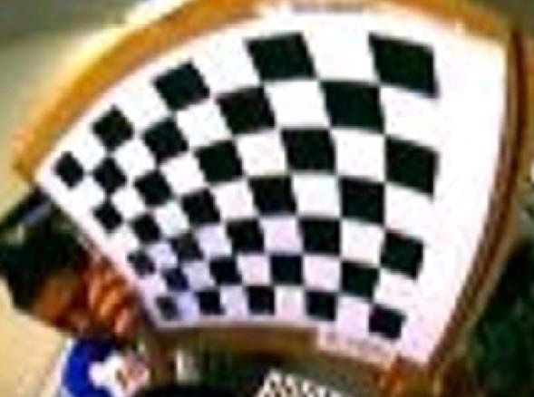
Here, the calibration is performed by using a half- tively in the catadioptric and dioptric case) is visible in
cylindrical calibration pattern perpendicular to the the image. Moreover, we assume that the image forma-
camera sensor, which rotates on a turntable. tion function, which manages the projection of a 3D
In [8, 10], the authors treat the case of a parabolic real point onto a pixel of the image plane, can be de-
mirror. In [8] it is shown that vanishing points lie on a scribed by a Taylor series expansion. The expansion
conic section which encodes the entire calibration coefficients, which constitute our calibration parame-
information. Thus, projections of two sets of parallel ters, are estimated by solving a two-step least-squares
lines suffice for intrinsic calibration. However, this linear minimization problem. Finally, the order of the
property does not apply to non-parabolic mirrors. series is determined by minimizing the reprojection
Therefore, the proposed technique cannot be easily error of the calibration points.
generalized to other kinds of sensors. The proposed procedure does not require any expen-
Conversely, the methods described in [10, 11, 12, sive equipment. Moreover, it is very fast and com-
14] fall in the self-calibration category. These methods pletely automatic, as the user is only requested to col-
require no calibration pattern, nor a priori knowledge lect a few images of the calibration pattern. The
about the scene. The only assumption is the capability method was applied to a KAIDAN 360° One VR sin-
to automatically find point correspondences in a set of gle-viewpoint mirror mounted on a CCD camera. The
panoramic images of the same scene. Then, calibration system has a vertical view angle greater than 200° and
is directly performed by epipolar geometry by mini- the image size is 900x1200 pixels. After calibration,
mizing an objective function. In [10, 12], this is done we obtained an average reprojection error of 1 pixel. In
by employing a parabolic mirror, while in [11, 14] a order to test the accuracy of the method, we used the
fish-eye lens with a view angle greater than 180° is estimated model in a structure from motion problem,
used. However, besides focusing on particular sensor and we obtained a 3D metric reconstruction of a scene
types, the mentioned self-calibration techniques may from two highly distorted omnidirectional images, by
suffer in case of tracking difficulties and of a small using image correspondences only.
number of features points [16]. The structure of the paper is the following. The omni-
All previous calibration procedures focus on par- directional camera model and calibration are described
ticular sensor types, such as parabolic and hyperbolic in Sec. 2 and 3. The results of the calibration of a real
mirrors or fish-eye lenses. Furthermore, they are system are given in Sec. 4. Finally, the 3D structure
strongly dependent on the omnidirectional sensor from motion experiment and its accuracy are shown
model they use, which is suitable only when the single and discussed in Sec. 5.
effective viewpoint property is satisfied. Although
several panoramic vision systems exist directly manu- 2. Omnidirectional Camera Model
factured to have this property, for a catadioptric system
this requires to accurately align the camera and the We want to generalize our procedure to different
mirror axes. In addition, the focus point of the mirror kinds of single-viewpoint omnidirectional vision sys-
has to coincide with the camera optical center. Since it tems, both catadioptric and dioptric. In this section we
is very difficult to avoid camera-mirror misalignments, will use the notation given in [11].
an incorrectly aligned catadioptric sensor can lead to a In the general omnidirectional camera model, we
quasi single-viewpoint optical system [2]. As a result, identify two distinct references: the camera image
the sensor model used by the mentioned techniques plane (u' , v' ) and the sensor plane (u' ' , v ' ' ) . In Fig. 1 the
could be suboptimal. In the case of fish-eye lenses the two reference planes are shown in the case of a catadi-
discussion above is analogue. optric system. In the dioptric case, the sign of u’’
Motivated by this observation, we propose a calibra- would be reversed because of the absence of a reflec-
tion procedure which uses a generalized parametric tive surface. All coordinates will be expressed in the
model of the sensor, which is suitable to different coordinate system placed in O, with the z axis aligned
kinds of omnidirectional vision systems, both catadiop- with the sensor axis (see Fig. 1a).
tric and dioptric. The proposed method requires the Let X be a scene point. Then, assume u' ' [u' ' , v ' ' ]T
camera to observe a planar pattern shown at a few
be the projection of X onto the sensor plane, and
different locations. Either the camera or the planar
u' [u ' , v ' ]T its image in the camera plane (Fig. 1b and
pattern can be freely moved. No a-priori knowledge of
the motion is required, nor a specific model of the 1c). As observed in [11], the two systems are related
omnidirectional sensor. The developed procedure is by an affine transformation, which incorporates the
based on the assumption that the circular external digitizing process and small axes misalignments; thus
boundary of the mirror or of the fish-eye lens (respec- u' ' Au' t , where A 2 x 2 and t 2 x1 . Then, let us
Proceedings of the Fourth IEEE International Conference on Computer Vision Systems (ICVS 2006)
0-7695-2506-7/06 $20.00 © 2006 IEEE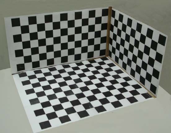
introduce the image projection function g, which cap- f u'',v''
2 N
a 0 a1 U ,, a 2 U ,, ... a N U ,, , (3)
tures the relationship between a point u' ' , in the sensor
plane, and the vector p emanating from the viewpoint where the coefficients a i , i 0, 1, 2, ...N , and the poly-
O to a scene point X (see Fig. 1a). By doing so, the
complete model of an omnidirectional camera is nomial degree N are the model parameters to be de-
termined by the calibration; U ,, ! 0 is the metric dis-
Op O g u' ' O g Au' t PX , O ! 0 , (1) tance from the sensor axis. Thus, (1) can be rewritten
as
where X 4 is expressed in homogeneous coordi-
nates; P 3x4 is the perspective projection matrix. By ªu ' ' º
ª Au' t º
calibration of the omnidirectional camera we mean the O ««v ' ' »» O g Au' t O« » P X , O ! 0 (4).
«¬ w' '»¼ ¬ f u' ' , v' ' ¼
estimation of the matrices A and t, and the non-linear
function g, so that all vectors g Au' t satisfy the
projection equation (1). This means that, once the 3. Camera Calibration
omnidirectional camera is calibrated, we are able to
reconstruct, from each pixel, the direction of the corre- By calibration of an omnidirectional camera we
sponding scene point in the real world. We assume for mean the estimation of the parameters [A,
g the following expression t, a 0 , a1 , a 2 ,..., a N ] so that all vectors g Au' t satisfy the
equation (4). In order to reduce the number of parame-
g u'',v''
T
u'',v'' , f u'',v'' , (2) ters to be estimated, we compute the matrices A and t,
up to a scale factor Į , by transforming the view field
where f is rotationally symmetric with respect to the ellipse (see Fig. 1c) into a circle centered on the ellipse
sensor axis. For instance, in the catadioptric case, this center. This transformation is calculated automatically
corresponds to assume that the mirror is perfectly by using an ellipse detector if the circular external
symmetric with respect to its axis. In general, such an boundary of the sensor is visible in the image. After
assumption is highly reasonable because both mirror performing the affine transformation, an image
profiles and fish-eye lenses are manufactured with point u' is related to the corresponding point on the
micrometric precision. sensor plane u' ' by u' ' D u' . Thus, by substituting
this relation in (4) and using (3), we have the following
projection equation
(5)
ªu' ' º ª D u' º ª u' º
« »
O ««v' ' »» O g D u' O «« D v' »» O D « v' » P X,
«¬w' '»¼ «¬ f D U' »¼ «a ... a U'N »
¬0 ¼
(a) (b) (c)
N
Figure 1. (a) Coordinate system in the catadi- O,D ! 0
optric case. (b) Sensor plane, in metric coor-
dinates. (c) Camera image plane, expressed in where now u ' and v ' are the pixel coordinates of an
pixel coordinates. (b) and (c) are related by an image point with respect to the circle center, and U ' is
affine transformation. the Euclidean distance. Also, note that the factor Į can
be directly integrated in the depth factor O ; thus, only
Function f can have various forms related to the N+1 parameters ( a 0 , a1 , a 2 ,..., a N ) need to be estimated.
mirror or the lens construction [12, 13, 14]. As men- During the calibration procedure, a planar pattern
tioned in the introduction, we want to apply a general- of known geometry is shown at different unknown
ized parametric model of f , which is suitable to differ- positions, which are related to the sensor coordinate
ent kinds of sensors. Moreover, we want this model to system by a rotation matrix R [ r1 , r2 , r3 ] and a transla-
compensate for any misalignment between the focus tion t, called extrinsic parameters. Let I i be an
point of the mirror (or the fish-eye lens) and the cam- observed image of the calibration pat-
era optical center. We propose the following polyno- tern, M ij [ X ij , Yij , Z ij ] the 3D coordinate of its points in
mial form for f
the pattern coordinate system, and mij [uij , vij ]T the
Proceedings of the Fourth IEEE International Conference on Computer Vision Systems (ICVS 2006)
0-7695-2506-7/06 $20.00 © 2006 IEEE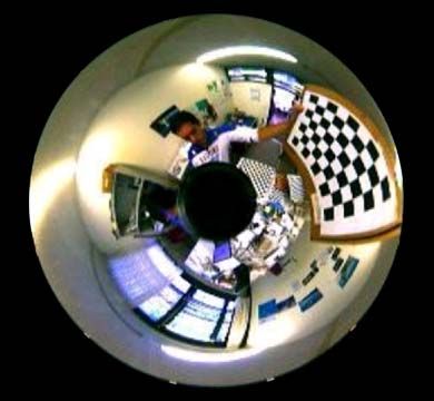
correspondent pixel coordinates in the image plane. r11 , r12 , r21 , r22 , t1 , t 2 . Thus, by stacking all the unknown
Since we assumed the pattern to be planar, without loss entries of (8.3) into a vector, we rewrite the equation
of generality we have Z ij 0 . Then, equation (5) be- (8.3) for L points of the calibration pattern as a system
comes of linear equations
(6)
ª uij º M H 0, (9)
« » i where
Oij pij Oij « vij » P X
« H [ r11 , r12 , r21 , r22 , t1 , t 2 ]T ,
N»
«¬a0 ... aN Uij »¼ and
ª v1 X 1 v1Y1 u1 X 1 u1Y1 v1 u1 º
ª Xij º M « : : : : : : »
« » ª Xij º « »
Y « » «¬ v L X L v LYL uL X L uLYL vL uL »¼
> @
r1i r2i r3i t i « ij »
«0 »
> 1
i
2
i
r r t «Yij » i
@
« » «1 »
¬ ¼ A linear estimate of H can be obtained by minimiz-
¬«1 ¼»
2
ing the least-squares criterion min M H , subject to
Therefore, in order to solve for camera calibration, the H
2
1 . This is accomplished by using the SVD.
extrinsic parameters have to be determined for each
pose of the calibration pattern. The solution of (9) is known up to a scale factor,
which can be determined uniquely since vec-
3.1. Solving for camera extrinsic parameters tors r1 , r2 are orthonormal. Because of the orthonormal-
ity, the unknown entries r31 , r32 can also be computed
Before describing how to determine the extrinsic uniquely.
parameters, let us eliminate the dependence from the To resume, the first calibration step allows finding
depth scale Oij . This can be done by multiplying both the extrinsic parameters r11 , r12 , r21 , r22 , r31 , r32 , t1 , t 2 for each
sides of equation (6) vectorially by pij pose of the calibration pattern, except for the transla-
tion parameter t 3 . This parameter will be computed in
ª X ij º the next step, which concerns the estimation of the
« » image projection function.
Oij p ij p ij p ij r > 1
i
r
2
i i
@
t «Yij » 0
«1 »
¬ ¼ 3.2. Solving for camera intrinsic parameters
ª º
. (7)
u ij ª X ij º
« » « » In the previous step, we exploited equation (8.3) to
« v ij i i
» r1 r2 t>i
@
«Yij » 0 find the camera extrinsic parameters. Now, we substi-
« N » «1 »
¬«a 0 ... a N U ij ¼» ¬ ¼ tute the estimated values in the equations (8.1) and
(8.2), and solve for the camera intrinsic parameters
a 0 , a1 , a 2 ,..., a N that describe the shape of the image
Now, let us focus on a particular observation of the
calibration pattern. From (7), we have that each projection function g. At the same time, we also com-
point p j on the pattern contributes three homogeneous pute the unknown t 3i for each pose of the calibration
equations pattern. As done above, we stack all the unknown
entries of (8.1) and (8.2) into a vector and rewrite the
v j ( r31 X j r32Y j t3 ) f ( U j ) ( r21 X j r22Y j t2 ) 0 (8.1) equations as a system of linear equations. But now, we
incorporate all K observations of the calibration rig.
We obtain the following system
f ( U j ) ( r11 X j r12Y j t1 ) u j ( r31 X j r32Y j t3 ) 0 (8.2)
(10)
N ª a0 º
u j ( r21 X j r22Y j t2 ) v j ( r11 X j r12Y j t1 ) 0 (8.3) ª A1 A1 U 1 .. A1 U 1 v1 0 .. 0 º « » ª B1 º
« » : «D »
0 » « »
N
« C1 C1 U 1 .. C1 U 1 . u1 0 .. « 1»
«a N »
« : : .. : : : .. : »« 1 » « : »
« N » « t3 » « »
Here X j , Y j and Z j are known, and so are u j , v j . Also, « AK AK U K .. AK U K 0 0 .. vK » « » « BK »
«C :
u K »¼ « K » «¬ D K »¼
N
¬ K CK U K .. C K U K 0 0 ..
observe that only (8.3) is linear in the unknown «¬ t 3 »¼
Proceedings of the Fourth IEEE International Conference on Computer Vision Systems (ICVS 2006)
0-7695-2506-7/06 $20.00 © 2006 IEEE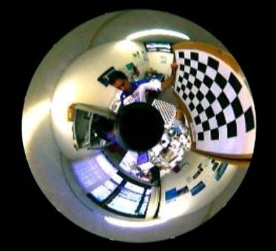
where calibration points onto the images. Then, we compute
the Root of Mean Squared Distances (RMS), in pixels,
Ai r21i X i r22i Y i t 2i , Bi vi ( r31i X i r32i Y i ) , between the detected image points and the reprojected
Ci r11i X i r12i Y i t1i and Di u i ( r31i X i r32i X i ) . ones. The calculated RMS values versus the number of
images are plotted in Fig. 3 for different polynomial
degrees. Note that the error decreases when more im-
Finally, the least-squares solution of the overdeter-
ages are used. Moreover, by using a 4th order polyno-
mined system is obtained by using the pseudoinverse.
mial to fit the model, we obtain the minimum RMS
Thus, the intrinsic parameters a 0 , a1 , a 2 ,..., a N , which
value, that is of about 1.2 pixels. A 3rd order polyno-
describe the model, are now available. In order to mial also provides a similar performance if more than
compute the best polynomial degree N, we actually four images are taken. Conversely, by using a 2nd order
start from N=2. Then, we increase N by unitary steps expansion, the RMS remains above 2 pixels. Thus, for
and we compute the average value of the reprojection our applications we used a 4th order expansion. As a
error of all calibration points. The procedure stops result, the RMS error of all reprojected calibration
when a minimum error is found. points is 1.2 pixels. This value is very good if we con-
sider that the image resolution is 900x1200 pixels, and
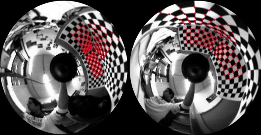
4. Experimental Results that corner detection is less precise on omnidirectional
images than on conventional perspective pictures. In
The calibration algorithm presented in the previous Fig. 4 you can see several corner points used to per-
sections was tested on real data. The omnidirectional form the calibration, and the same points reprojected
sensor to be calibrated is a catadioptric system com- onto the image according to the intrinsic and extrinsic
posed of a KAIDAN 360° One VR hyperbolic mirror parameters estimated by the calibration.
and a SONY CCD camera having a resolution of
900x1200 pixels. The calibration rig is a checker pat-
tern containing 9x7 squares, so there are 48 corners 7,00
(calibration points) (see Fig. 4). The size of the pattern 6,00
5,00
is 24.3cm x 18.9 cm. Eleven images of the plane under 4,00
different orientations were taken, some of which are 3,00
2,00
shown in Fig. 2. 1,00
0,00
2 3 4 5 6 7 8 9 10 11
Figure 3. RMS error versus the number of
images of the pattern. The RMS values are
computed for different polynomial degrees:
2nd order (black u ), 3rd order (blue x ) and 4th
order (red $ ).
Figure 2. Some images of the calibration pat-
tern taken under different orientations
4.1. Performance with respect to the number of
planes and the polynomial degree
This experiment investigates the performance of our
technique with respect to the number of images of the Figure 4. The corner points used for calibra-
planar pattern, for a given polynomial degree. We vary tion (red crosses) and the reprojected ones
the number of pictures from 2 to 11, and for each set (yellow rounds) after calibration.
we perform the calibration. Next, according to the
estimated extrinsic parameters, we reproject the 3D
Proceedings of the Fourth IEEE International Conference on Computer Vision Systems (ICVS 2006)
0-7695-2506-7/06 $20.00 © 2006 IEEE
pattern in the original image (Fig. 6) appear straight
             4.2. Performance with respect to the noise level                                after rectification (Fig. 7).

                In this experiment, we study the robustness of our                           5. Application to Structure from Motion
             calibration technique in case of inaccuracy in detecting
             the calibration points. At this end, Gaussian noise with                           Our work on omnidirectional camera calibration is
             mean 0 and standard deviation V is added to the input                           motivated by the use of panoramic vision sensors for
             calibration points. We vary the noise level from 0.1                            structure from motion and 3D reconstruction. In this
             pixels to 1.5 pixels. For each level, we perform the                            section, we perform a 3D metric reconstruction of a
             calibration and we compute the RMS error of the re-                             real object from two omnidirectional images, by using
             projected points. The results obtained using a 4th order                        the sensor model estimated by our calibration proce-
             polynomial are shown in Fig. 5. As it can be seen, the                          dure. In order to compare the reconstruction results
             RMS values remain under 2 pixels.                                               with a ground truth, we exploited a trihedral object
                                                                                             composed of three orthogonal checker patterns of
                         2,0
                                                                                             known geometry (see Fig. 8).
                         1,9
                         1,8
                         1,7
                         1,6
                         1,5
                         1,4
                         1,3
                         1,2
                         1,1
                         1,0
                               0,1 0,2 0,3 0,4 0,5 0,6 0,7 0,8 0,9 1,0 1,1 1,2 1,3 1,4 1,5

             Figure 5. RMS error versus the noise level.

                                                                                             Figure 8. The sample trihedron used for the
                                                                                             3D reconstruction experiment.

                                                                                             Two images of the trihedron were taken by positioning
                                                                                             our calibrated camera at two unknown different loca-
                                                                                             tions (see Fig. 9). Then, several point matches were
                                                                                             picked manually from both views of the object and the
                                                                                             eight point algorithm [17] was applied. In order to
             Figure 6. A sample                               Figure 7. The sample
                                                                                             obtain good reconstruction results, more than eight
             image before rectifi-                            image of Fig. 6 after
                                                                                             points (actually 135) were extracted. Then, the coordi-
             cation.                                          rectification. Now the
                                                                                             nates of the correspondent 3D vectors, back-projected
                                                              edges (highlighted)
                                                                                             into the space, were normalized according to the non-
                                                              appear straight.
                                                                                             uniform mirror resolution. The results of the recon-
                                                                                             struction are shown in Fig. 10, where we used checker
             4.3. Performance with respect to image rectifi-                                 patches to fit the reconstructed 3D points (red rounds).
             cation                                                                          In order to compare the results with the ground truth,
                                                                                             we computed the angles between the three planes fit-
                In this experiment, we test the accuracy of the esti-                        ting the reconstructed points. We found the following
             mated sensor model by rectifying all calibration im-                            values: 94.6°, 86.8° and 85.3°. Moreover, the average
             ages. Rectification determines a transformation of the                          distances of these points from the fitted planes were
             original distorted image such that the new image ap-                            respectively 0.05 cm, 0.75 cm and 0.07 cm. Finally,
             pears as taken by a conventional perspective camera.                            since we knew the size of each checker to be 6.0 cm x
                In general, is impossible to rectify the whole omni-                         6.0 cm, we also calculated the dimension of every
             directional image because of a view field larger than                           reconstructed checker, and we found an average error
             180°. However, it is possible to perform rectification                          of 0.29 cm.
             on image regions which cover a smaller field of view.
             As a result, linearity is preserved in the rectified image.
             As you can see in Fig. 6, curved edges of a sample

Proceedings of the Fourth IEEE International Conference on Computer Vision Systems (ICVS 2006)
0-7695-2506-7/06 $20.00 © 2006 IEEE
two-step least-squares linear minimization problem. To
test the proposed technique, we calibrated a panoramic
camera having a field of view greater than 200° in the
vertical direction, and we obtained very good results.
To investigate the accuracy of the calibration, we also
used the estimated omni-camera model in a structure
from motion experiment. We obtained a 3D metric
reconstruction of a real object from two omnidirec-
tional images, by using image correspondences only.
The reconstruction results were also compared with the
ground truth. With respect to classical techniques,
Figure 9. Two pictures of the trihedron taken which rely on a specific parametric model of the omni-
by the omnidirectional camera. The points directional camera, the proposed procedure is inde-
used for the 3D reconstruction are indicated pendent of the sensor, easy to use and flexible.
by red dots.
7. References
[1] Baker, S. and Nayar, S.K. “A theory of catadioptric
image formation”. In Proceedings of the IEEE Interna-
tional Conference on Computer Vision (ICCV’98),
Bombay, India, 1998, pp. 35–42.
[2] R. Swaminathan, M. D. Grossberg, and N. S. K. “Caus-
tics of catadioptric cameras”. In Proceedings of the
IEEE International Conference on Computer Vision
(ICCV’01), Vancouver, Canada, 2001.
[3] B.Micusik, T.Pajdla. “Autocalibration & 3D Recon-
struction with Non-central Catadioptric Cameras”. In
Proceedings of International Conference on Computer
Vision and Pattern Recognition (CVPR’04), Washing-
ton US, 2004.
[4] S. Baker and S. Nayar. “A theory of single-viewpoint
catadioptric image formation”. International Journal of
Computer Vision, 35(2), November 1999, pp. 175–196.
[5] C. Cauchois, E. Brassart, L. Delahoche, and T. Del-
hommelle. “Reconstruction with the calibrated syclop
sensor”. In Proceedings of the IEEE International Con-
ference on Intelligent Robots and Systems (IROS’00),
Takamatsu, Japan, 2000, pp. 1493–1498.
[6] T. Svoboda, T. Pajdla, and V. Hlavac. “Central pano-
Figure 10. Three rendered views of the recon- ramic cameras: Geometry and design”. Research report.
structed trihedron. Note that the object was Czech Technical University - Center for Machine Per-
reconstructed only from two highly distorted ception, Praha, Czech Republic, December 1997.
omnidirectional images (as in Fig. 9). [7] H. Bakstein and T. Pajdla. “Panoramic mosaicing with
a 180ƕ field of view lens”. In Proceedings of the IEEE
Workshop on Omnidirectional Vision, 2002, pp. 60–67.
6. Conclusions [8] C. Geyer and K. Daniilidis. “Paracatadioptric camera
calibration”. PAMI, 24(5), May 2002, pp. 687-695.
In this paper, we presented a flexible new technique [9] J. Gluckman and S. K. Nayar. “Ego-motion and omni-
for single-viewpoint omnidirectional camera calibra- directional cameras”. In Proceedings of the IEEE Inter-
tion. The proposed method only requires the camera to national Conference on Computer Vision (ICCV’98),
observe a planar pattern shown at a few different ori- Bombay, India, 1998, pp. 999-1005.
[10] S. B. Kang. “Catadioptric self-calibration”. (CVPR’00),
entations. No a-priori knowledge of the motion is re-
2000, pp. 201-207.
quired, nor a specific model of the omnidirectional [11] B. Micusik and T. Pajdla. “Estimation of omnidirec-
sensor. The only assumption is that the image projec- tional camera model from epipolar geometry”. In Proc.
tion function can be described by a Taylor series ex- of CVPR’03, 2003, pp. 485.490.
pansion whose coefficients are estimated by solving a
Proceedings of the Fourth IEEE International Conference on Computer Vision Systems (ICVS 2006)
0-7695-2506-7/06 $20.00 © 2006 IEEE[12] B.Micusik, T.Pajdla. “Para-catadioptric Camera Auto-
calibration from Epipolar Geometry”. ACCV 2004, Ko-
rea, January 2004.
[13] J. Kumler and M. Bauer. “Fisheye lens designs and
their relative performance”.
[14] B.Micusik, D.Martinec, T.Pajdla. “3D Metric Recon-
struction from Uncalibrated Omnidirectional Images”.
ACCV’04, Korea, (January 2004).
[15] T. Svoboda, T.Pajdla. “Epipolar Geometry for Central
Catadioptric Cameras”. IJCV, 49(1), Kluwer, August
2002, pp. 23-37.
[16] S. Bougnoux. “From projective to Euclidean space
under any practical situation, a criticism of self-
calibration”. In Proceedings of the 6th International
Conference on Computer Vision, Jan. 1998, pp. 790–
796.
[17] H.C. Longuet-Higgins. “A computer algorithm for
reconstructing a scene from two projections”. Nature,
Sept 1981, 293:133–135.
[18] R. I. Hartley. “In defence of the 8-point algorithm”. In
Proceedings of the IEEE International Conference on
Computer Vision (ICCV’95), 1995.
[19] Y. Ma, S. Soatto, J. Kosecka, S. Sastry, “An invitation
to 3D vision, from images to geometric models mod-
els”, Springer Verlag, ISBN-0-387-00893-4. 2003.
[20] Q.-T. Luong and O. Faugeras. “Self-calibration of a
moving camera from point correspondences and fun-
damental matrices”. The International Journal of Com-
puter Vision, 22(3), 1997, pp. 261–289.
[21] Zhengyou Zhang. “A Flexible New Technique for
Camera Calibration”, IEEE Transactions on Pattern
Analysis and Machine Intelligence, Volume 22, Issue
11, November 2000, pp.: 1330 – 1334.
Proceedings of the Fourth IEEE International Conference on Computer Vision Systems (ICVS 2006)
0-7695-2506-7/06 $20.00 © 2006 IEEEYou can also read