Industrial Electrical Energy Consumption Forecasting by using Temporal Convolutional Neural Networks
←
→
Page content transcription
If your browser does not render page correctly, please read the page content below
MATEC Web of Conferences 335, 02003 (2021)                            https://doi.org/10.1051/matecconf/202133502003
14th EURECA 2020

      Industrial Electrical Energy Consumption
      Forecasting by using Temporal Convolutional
      Neural Networks
      Kai Lok Lum1, Hou Kit Mun1,*, Swee King Phang1 and Wei Qiang Tan2
      1Taylor’s University, 1, Jalan Taylors, 47500 Subang Jaya, Selangor, Malaysia
      2GoAutomate   Sdn Bhd, 33, Jalan Pentadbir U1/30, Taman Perindustrian Batu 3, 40150 Shah Alam,
      Selangor, Malaysia

                    Abstract. In conjunction with the 4th Industrial Revolution, many
                    industries are implementing systems to collect data on energy consumption
                    to be able to make informed decision on scheduling processes and
                    manufacturing in factories. Companies can now use this historical data to
                    forecast the expected energy consumption for cost management. This
                    research proposes the use of a Temporal Convolutional Neural Network
                    (TCN) with dilated causal convolutional layers to perform forecasting
                    instead of conventional Long-Short Term Memory (LSTM) or Recurrent
                    Neural Networks (RNN) as TCN exhibit lower memory and computational
                    requirements. This approach is also chosen due to traditional regressive
                    methods such as Autoregressive Integrated Moving Average (ARIMA)
                    fails to capture non-linear patterns and features for multi-step time series
                    data. In this research paper, the electrical energy consumption of a factory
                    will be forecasted by implementing a TCN to extract the features and to
                    capture the complex patterns in time series data such daily electrical energy
                    consumption with a limited dataset. The neural network will be built using
                    Keras and TensorFlow libraries in Python. The energy consumption data as
                    training data will be provided by GoAutomate Sdn Bhd. Then, the
                    historical data of economic factors and indexes such as the KLCI will be
                    included alongside the consumption data for neural network training to
                    determine the effects of the economy on industrial energy consumption.
                    The forecasted results with and without the economic data will then be
                    compared and evaluated using Weighted Average Percentage Error
                    (WAPE) and Mean Absolute Percentage Error (MAPE) metrics. The
                    parameters for the neural network will then be evaluated and fined tuned
                    accordingly based on the accuracy and error metrics. This research is able
                    create a CNN to forecast electrical energy consumption with WAPE =
                    0.083 & MAPE = 0.092, of a factory one (1) week ahead with a small scale
                    dataset with only 427 data points, and has determined that the effects of
                    economic index such as the Bursa Malaysia has no meaningful impact on
                    industrial energy consumption that can be then applied to the forecasting of
                    energy consumption of the factory.

      *
          Corresponding author: houkit.mun@taylors.edu.my

© The Authors, published by EDP Sciences. This is an open access article distributed under the terms of the Creative Commons
Attribution License 4.0 (http://creativecommons.org/licenses/by/4.0/).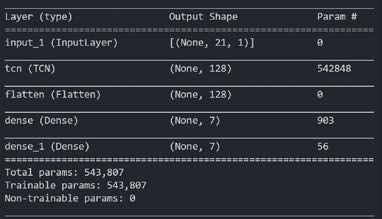
MATEC Web of Conferences 335, 02003 (2021)                        https://doi.org/10.1051/matecconf/202133502003
14th EURECA 2020

     1 Introduction
     An accurate electrical energy consumption forecast is vital to manufacturing industries to
     run their operations via managing and planning of energy policy [1], operational schedules
     and manufacturing processes as industrial sectors. According to the Malaysian Energy
     Commission as the industrial sector alone in Malaysia has consumed over 71 million
     kilowatt-hours in 2017 [2]. One of the main reasons is due to the high cost associated with
     operating the industrial machines required in the production line which is consuming large
     amounts of electrical energy and directly translates to higher electricity costs. Hence, the
     operational times of these machines in the production lines need to be planned in advance
     to ensure a high efficiency in balancing time, cost and production output [3].Traditionally,
     common methods for electrical forecasting purposes typically include regression analysis
     such as Support Vector Machines (SVM) and Least Squares Support Vector Machines
     (LSVM) as utilized by Kaylez et al.[4] and using (ARIMA) algorithm as built by
     Nichiforov et al. for electrical forecasting. However, electrical energy consumption as time
     series data forecast represents a difficult type of predictive modelling problem due to the
     existence of complex linear and non-linear patterns [5].
            Some researchers proposed artificial neural networks for forecasting electrical consumption. Li
     et.al used Convolutional Neural Networks (CNN) with the time-series data of electrical consumption
     for energy forecasting without considering external factors such as the weather and economy [6].
     However, it is shown that too many input variables by considering of many different external factors
     can lead to invalid results by complicating the prediction and training process of the neural network
     [7]. Hence, this research aims to rectify this problem by only selecting economic factors as the sole
     external factor that will have a significant impact on electrical energy consumption.
     Although most of the previously proposed methods for electrical energy consumption forecasting had
     promising and accurate results but they need to use a large data sets ranging from over 257 thousand
     records [6] to 1.4 million records [4] for forecasting. Reliable large data sets are only accessible if the
     data is available through public domain or companies has already built in infrastructures for data
     collection. As implementing such infrastructures on top of a manufacturing production line is costly,
     most small-medium enterprises (SME) may not have the capability to implement the data collection
     and monitoring infrastructure yet or may not even have the capability or financial prowess to maintain
     the system altogether. Therefore, the current data that has been collected by SME are much more
     limited compared to large enterprises. Based on the feature extraction performance of CNN [8],
     shows that it is able extract the features and capture the hidden dynamics of the time-series data and
     able to generate predictions [9]. As times-series data are sequential and temporal, a method to ensure
     that there is no leakage of information from future time steps in the sequence is to ensure that the
     convolutional layers in the network to be causal. Causal convolution is different from standard
     convolution due to convolutional operation performed to obtain the output does not take future values
     as inputs [11]. This architecture of CNNs are named as Temporal Convolutional Neural Network
     (TCN) as it is especially suited to handle temporal time-series data.
     Therefore, this research is proposed to create an optimized TCN to forecast the electrical energy
     consumption of a SME’s factory with small data set.

     2 Methodology
     In this section, the methods to create a Temporal Convolutional Neural Network and
     optimize the performance of the network with limited training data set will be discussed.
     Visual Studio Code is used as the main code editing program that is used for this project,
     while Microsoft Excel is used to tabulate the data of the results.

     2.1 Data acquisition & preprocessing

                                                         2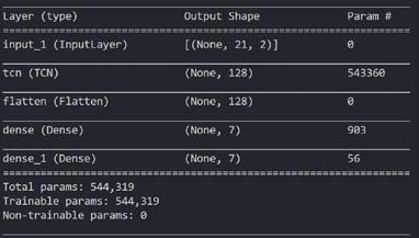
MATEC Web of Conferences 335, 02003 (2021) https://doi.org/10.1051/matecconf/202133502003
14th EURECA 2020
To acquire the data for training, a custom Node.js script is written to download the import the raw
data as captured by the sensors in the factory is uploaded to Firestore [12]. Firestore is a NoSQL
cloud database to store data and server development from Firebase and the Google Cloud Platform. A
Firebase service account is registered with permission from GoAutomate Sdn Bhd, and an
authentication token is generated to authorize the manipulation of the database from an external
script. The Node.js script implements a custom algorithm to segregate and calculate daily energy
consumption from the cumulative raw data in (kWh) kilowatt-hour unit provided by the sensors as the
data is sampled every 5 minutes. The downloaded energy consumption data is then normalized with
z-score normalization to improve convergence of deep learning neural networks. Z-score
normalization is a strategy of normalizing data that avoid any outlier data related issues. The formula
for z-score normalization is shown below.
(1)
Where is the actual value, is the mean and is the standard deviation.
The economic index that is chosen for economic factors is the Bursa Malaysia Kuala Lumpur
Composite Index or Kuala Lumpur Stock Exchange (KLSE) as it is a daily index that is able to reflect
the condition and state of economy of the nation.
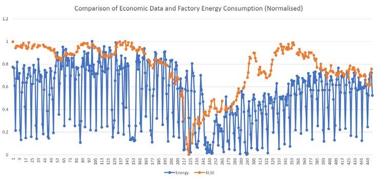
Fig. 1. Normalized comparison of economic index and electrical energy consumption
As seen in the figure above, it can be seen that there are correlation between the trend of the KLSE
and electrical energy consumption of the factory.
2.2 Input-output pair sliding window method
As the outcome of the project is to output a multi-time step forecast, that is 7 days of forecasted
electrical energy usage, a multi-input multi-output (MIMO) architecture is selected for the network
instead of recursive approaches such as forecasting a single timestep, then feedback the last forecast
as input for the next forecast as recursive approaches tend to accumulate errors over several forecasts
for multi-step prediction [13].
As a result, the training data will be reshaped into the form of a pair input-output sequences. The
input-output sequence pairs will follow a sliding window scheme across the entire raw training data to
be created. For example, the output sequence in this scenario has a length of 7, while the input
sequence is preliminarily chosen as 21. As such, the network will use a lookback window of 21 days
3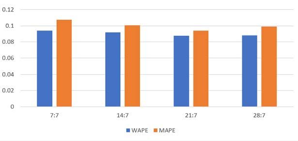
MATEC Web of Conferences 335, 02003 (2021)                       https://doi.org/10.1051/matecconf/202133502003
14th EURECA 2020

     as an input to generate a forecast of the next 7 days as output. To help illustrate the sliding window
     scheme to generate input-output sequence pair, an example figure is shown below.

     Fig. 2. Example of input-output sequence pair generation with sliding window method.
     The training data for the TCN only consists of electrical energy consumption data from August 1,
     2019 – September 14, 2020 with a relatively small dataset of only 424 values. The generation of
     input-output sequence pair with sliding window method is implemented using a script in Python with
     the utilization of the NumPy library.

     2.3 Forecast accuracy metrics
     The accuracy of the forecasted values in the output sequence will be evaluated using Weighted
     Average Percentage Error (WAPE), Mean Average Percentage Error (MAPE) and Root Mean Square
     Error (RMSE) metrics.

                                  n

                     WAPE =
                            ∑     i =1
                                         actuali − forecasti                                        (2)
                                            n
                                         ∑i=1 actuali

                                1 n actual i − forecast i
                     MAPE =       ∑
                                n i =1    actual i
                                                                                                     (3)

     where n is the length of the network output or forecast window.

     3 Results and Discussion

     3.1 Temporal convolutional network parameters
     To ensure reproducibility and uniformity to the project, a seed for the training process of the neural
     network is fixed as it is a built-in function of the Keras-TensorFlow library. The TCN is trained with
     training data as prepared as input-output pair batch size of 7, with starting with and arbitrarily number

                                                           4
MATEC Web of Conferences 335, 02003 (2021) https://doi.org/10.1051/matecconf/202133502003
14th EURECA 2020
of 30, then varying epochs/iterations to determine most optimized configuration for most accurate
forecasts.
The fixed parameters of the TCN are as follows, dilations layers or nb_stacks=1,
padding='causal', return_sequences=False, dropout_rate=0.
The optimal network configurations are determined via a series of repeated testing by generating
models with different parameters and gauging the accuracy of the forecast using the error metrics of
WAPE and MAPE as stated previously. First, it has been determined that an epoch of 38 yields
optimum results via a test of several sets of testing data, obtaining the average MAPE and WAPE to
determine the optimum model configuration.
Table 1. Average error metrics of forecast with different epochs.
Test Set 1 (Week 1) Test Set 2 (Week 2)
Epochs MAPE WAPE Epochs MAPE WAPE
30 0.10556 0.098243 30 0.10094 0.09284
38 0.09390 0.08755 38 0.10058 0.09184
40 0.12070 0.11350 40 0.12984 0.11694
50 0.09666 0.09461 50 0.10640 0.09298
60 0.10668 0.10578 60 0.09461 0.09498
Test Set 3 (Week 3) Test Set 4 (Week 4)
Epochs MAPE WAPE Epochs MAPE WAPE
30 0.10855 0.09406 30 0.11091 0.09996
38 0.09899 0.08821 38 0.10751 0.09402
40 0.12510 0.10844 40 0.10595 0.09289
50 0.11805 0.10379 50 0.09164 0.07991
60 0.11678 0.09944 60 0.11741 0.10407
As it can be seen in Table 1 (in bold) that training for 38 epochs or iterations yields best overall
results for this set of factory electrical energy consumption data.
The optimum ratio for the input, lookback window and output, forecast window has been tested
and verified to be at 21:7, that is to have the network using a lookback window of 21 days as an input
to generate a forecast of the next 7 days as output. This is verified by repeated testing of 4 different
ratios of input-output window for the model with several sets of testing data and comparing the error
metrics. The comparison chart is shown below.
Fig. 3. Comparison of input-output window ratio for network.
5MATEC Web of Conferences 335, 02003 (2021) https://doi.org/10.1051/matecconf/202133502003
14th EURECA 2020
Once the optimum basic parameters for the network, that is the ratio of lookback window
(input), forecast window(output) and epoch are determined, other parameters to optimize the network
based on the MAPE & WAPE scores can be done.
Next, the configurations of 32, 64 and 128 convolutional filters (nb_filters) were tested on 4 sets of
testing data as stated previously. The optimum number of convolutional filters as tested is at 128. The
average value for error metrics is shown in the table below.
Table 2. Average error metrics of forecast for different number convolutional filters.
nb_filter Average WAPE Average MAPE
32 0.093896506 0.087554652
64 0.116039414 0.103804283
128 0.087554652 0.093896506
The activation function used for the network is the Rectified Linear Unit (ReLU) function in
order to overcome the vanishing gradient problem and is commonly used in convolutional neural
networks as it enables networks to learn faster. For the optimization function of the neural network,
the Adam algorithm instead of a conventional stochastic gradient descent (SGD) function. An
optimization function is a function that adjusts and configures the weights of the network after every
epoch/iteration during training. The configuration hyperparameters of the Adam are left as default as
per Keras-TensorFlow with learning_rate=0.001, beta1=0.9, beta2=0.999, epsilon=1e-08. Adam is
chosen due to the adaptive per-parameter learning rates based on the average of recent magnitudes of
the gradients for the weights.
The loss function used for the output is Mean Absolute Error (MAE) is used as it is commonly
used for regression problems by comparing absolute error between forecasted and actual values, and
works in tandem with the Adam optimizer to readjust the weights and biases in the network.
The padding of the TCN is ensured to be set at causal as to prevent any leakage of information from
the future to the past, and avoid creating a self-fulfilling forecasting model which does not accurately
model the electrical energy consumption of the factory.
After comparison between different major parameters of the TCN, a comparison of the
forecasted results of the network trained. The test data consists of an input sequence of 21 days of
electrical consumption and output sequence of 7 days. The TCN has not encountered or seen the data
before during training. The input sequence is fed into the network to generate the predicted output
sequence. The actual and forecasted results by TCN of different configurations are then evaluated and
compared.
Several sets of test input sequences, that are the electrical energy consumption of the factory of
21 days, will be fed into the network to generate a forecasted output sequence for the next 7 days. The
test data sets will be normalized before it is fed into the TCN. The TCN is tasked to generate a
forecast for several weeks for the month of October 2020, the testing sequences, input and output will
be tabulated below for each week. A visualization of the input-output sequences for all 4 weeks is
shown in Figure below.
(a) (b)
6MATEC Web of Conferences 335, 02003 (2021) https://doi.org/10.1051/matecconf/202133502003
14th EURECA 2020
(c) (d)
(e) (f)
(g) (h)
Fig. 4. Plot of (a) test input sequence, Sep 15 – Oct 5; b) test output sequence, Oct 6 – Oct 12; (c) test
input sequence, Sep 21 – Oct 11; (d) test output sequence, Oct 12 – Oct 18; (e) test input sequence,
Sep 27 – Oct 17; (f) test output sequence, Oct 18 – Oct 24; (g) test input sequence, Oct 3 – Oct 23; (h)
test output sequence, Oct 24 – Oct 30.
Finally, two different kernel sizes and dilations configurations were also compared. The
accuracy of the forecast results of the different configurations are tabulated below. The error metrics
used for evaluating forecast accuracy are generated with the aid of NumPy library.
7MATEC Web of Conferences 335, 02003 (2021) https://doi.org/10.1051/matecconf/202133502003
14th EURECA 2020
Table 3. Error metrics of forecast with kernel size of 2 and dilations of [1, 2, 4, 8, 16, 32, 64].
Week MAPE WAPE
1 0.0271148 0.0278651
2 0.149722 0.145305
3 0.076674 0.074936
4 0.122075 0.102113
Average 0.0938965 0.0875547
Table 4. Error metrics of forecast with kernel size of 3 and dilations of [1, 5, 7, 14, 28, 56]
Week MAPE WAPE
1 0.0836374 0.0747321
2 0.095645 0.101379
3 0.103627 0.088064
4 0.086349 0.066369
Average 0.0923144 0.0826359
The optimum model, is a TCN that is trained for 38 iterations, with a lookback window of
length 21, output window of length 7, with a batch size of 7, kernel size of 3 with dilations of [1 5 7
14 28 56 ], and with 128 convolutional filters. The average MAPE and WAPE are about 0.0923 and
0.0826 respectively.
The output of the neural network will then be denormalized based on the z-score normalization
parameters to obtain forecasted electrical energy consumption values in kWh (kilowatt-hour).
It should also be noted that the networks are able to capture features and trends such as the low
energy usage on weekends especially on Sundays, that is on Oct 11 where the TCN is able to forecast
as shown in the Figure 5(a), then back to a nominal higher energy usage on Mondays on Oct 12,
where weekdays have a higher usage of electrical energy at the factory due to resuming
manufacturing operations. This pattern is similarly observed as well in testing sets in other weeks on
Oct 18 to Oct 19 and again on Oct 25 to Oct 26.
(a) (b)
8MATEC Web of Conferences 335, 02003 (2021) https://doi.org/10.1051/matecconf/202133502003
14th EURECA 2020
(c) (d)
Fig. 5. Comparison of forecast of the best performing model and actual energy consumption values (a)
Week of Oct 6 – Oct 12 (b) Week of Oct 12 – Oct 18; (c) Week of Oct 18 – Oct 24; (d) Week of Oct
24 – Oct 30.
Another feature of interest is that the network is not trained on a strict weekend to weekend
fashion, and hence does not rely on a fixed pattern on starting of the week to the end of the week and
is able to predict with 90% accuracy from any day chosen in the week to generate a forecast of the
next 7 days. This can be seen in the results where all 4 sets of testing data start on different days in
Figure 5. The combined plot of forecasted and actual energy usage is shown in Figure 6.
Fig. 6. Combined plot of forecasted & actual energy usage.
3.2 Temporal convolutional network parameters
By factoring in the economic data into the optimum model based on previous testing, that is a neural
network that is trained for 38 iterations, kernel size of 3 with dilations of [1 5 7 14 28 56 ], and with
128 convolutional filters. The KLSE data is merged with the energy consumption data and trained in
the exact same parameters and methods. Most numerical operations are performed with the aid of
NumPy library.
As the KLSE does not have data on public holidays and weekends, interpolation is performed
on the KLSE dataset to obtain parity in data count with the energy consumption data of the factory.
Interpolation is performed using Microsoft Excel in Comma Separated Value (CSV) format. It can be
observed from the results of the economic it is apparent that the trends and features of the differing
weeks in the month of October has been successfully captured but is noticeably similar to the results
of the model without the economic factor.
9MATEC Web of Conferences 335, 02003 (2021) https://doi.org/10.1051/matecconf/202133502003
14th EURECA 2020
(a) (b)
(c) (d)
Fig. 6. Comparison of forecast of the best performing model and actual energy consumption values
with inclusion of economic factor. (a) Week of Oct 6 – Oct 12 (b) Week of Oct 12 – Oct 18; (c) Week
of Oct 18 – Oct 24; (d) Week of Oct 24 – Oct 30.
Table 5. Comparison of error metrics for forecasting energy with economic factor and without
economic factor.
With Economic Without Economic
Factor Factor
Week MAPE MAPE MAPE MAPE
1 0.0619923 0.0605042 0.0836374 0.0747321
2 0.0749508 0.0745891 0.095645 0.101379
3 0.1020385 0.1050175 0.103627 0.088064
4 0.131375 0.1225641 0.086349 0.066369
Average 0.0925893 0.0906687 0.0923144 0.0826359
Based on the results in Table 5, there is a degradation in both MAPE and WAPE scores as the
univariate model without economic factors still upholds the superior position of the optimal
configuration.
Although it can be observed that there are similar long term trends when visually and
numerically (after normalization) comparing both KLSE and the energy consumption of the factory,
the additional external economic factor does not have a huge impact on forecasting accuracy and
performance as the fluctuations of the KLSE indicator is too noisy on small scale, such as in this
project, to have any meaningful impact to aid in forecasting accuracy even if it exhibits similar trends
in comparison.
10MATEC Web of Conferences 335, 02003 (2021) https://doi.org/10.1051/matecconf/202133502003
14th EURECA 2020
In terms on computational efficiency, the inclusion of economic data increased the trainable
parameters as reported by TensorFlow by 20% as compared to models with only the electrical energy
consumption data. The model summary for both models is shown below.
(a) (b)
Fig. 7. Comparison of model summaries for each model (a) Model summary inclusive of KLSE; (b)
Model summary without economic data.
Table 6. Comparison of time taken to train and generate each model
Trainable Training Forecasting
MAPE WAPE
Parameters Time (s) Time (s)
Univariate
543, 807 0.0923145 0.082636 54.37 7.71
Model
Model with
economic 544, 319 0.104595 0.097026 57.98 8.03
factor
In the table above, it can be seen that not only the inclusion of economic factors
regressed the accuracy of the model, but it also decreased computational efficiency as the
parameters has increased resulting in a slower training and prediction time as tabulated in
Table 7. It can be concluded that the inclusion of economic data does not have any positive
or meaningful impact on forecasting accuracy for electrical energy consumption. The
models are all computed on the same hardware, that is an Intel Core i5-1035G4 CPU
without the use of a discrete graphics card. Due to the extra steps of data processing for
another set of data to be prepared in order to generate a forecast, it can be concluded that
the addition of economic factor decreases computational efficiency and worsens overall
performance of the model and is not recommended to be implemented.
4 Conclusion
Temporal Convolutional Neural Networks (TCN) are indeed feasible for forecasting electrical energy
consumption even with a limited dataset via causal dilated convolutional layers and resulting in
adequate forecasting accuracy with WAPE of 8.3% and MAPE of 9.2%. These results are achieved
by using the optimal configurations for the TCN. The optimal configurations for small dataset
forecasting modelling are determined to be at trained 38 epochs, with 128 convolutional filters, a
kernel size of 3 with 5 dilation layers of [1 5 7 14 28 56]. The inclusion of KLCI economic data did
not have a large effect on forecasting accuracy but has in fact regressed the performance of the
optimal model with WAPE of 9.7% and MAPE of 10.5% of. It can be concluded that KLCI data,
although likely to have correlation, is not suitable as the chosen index that is optimal external factor to
improve forecasting accuracy.
11MATEC Web of Conferences 335, 02003 (2021) https://doi.org/10.1051/matecconf/202133502003
14th EURECA 2020
Acknowledgement: The authors would like to acknowledge Taylor’s University for support for this
project. Authors would like to acknowledge GoAutomate Sdn Bhd. for providing access to electrical
energy consumption data of factory for this project.
References
1. M.-Acevedo, Energy Procedia. 57, 782 (2014).
2. "Electricity - Final Electricity Consumption", Malaysia Energy Information Hub.
[Online]. Doi: https://meih.st.gov.my/statistics. [Accessed: 13 Oct 2020].
3. M. Krones, E. Müller, Procedia CIRP. 17, 505 (2014).
4. F. Kaytez, M. Taplamacioglu, E. Cam, F. Hardalac, Int. J. Elec. Pow. Energy Sys. 67,
431 (2015).
5. C. Nichiforov, I. Stamatescu, I. Făgărăşan, G. Stamatescu, 5th Int Sym. Elect. Electron.
Eng. (ISEEE). 1 (2017).
6. L. Li, K. Ota, M. Dong, 14th Int. Sym. Perva. Sys. Alg. Net. & 11th Int. Conf. Fron.
Comp. Sci. Technol. & 3rd Int. Sym. Crea. Comp. 1 (2017).
7. F. Kaytez, M. Taplamacioglu, E. Cam, F. Hardalac, Int. J. Elec. Pow. Energy Sys. 67,
431 (2015).
8. Z. Horn, L. Auret, J. McCoy, C. Aldrich, B. Herbst, IFAC. 50, 13 (2017).
9. A. Adebiyi, A. Adewumi, C. Ayo, J. Appl. Math. 1 (2014).
10. A. van de Oord, S. Dieleman, H. Zen, K. Simonyan, O. Vinyals, A. Graves, N.
Klachbrenner, A. Senior, K. Kvukcuoglu. “WaveNet: A Generative Model For Raw
Audio”. arXiv preprint arXiv:1609.03499. (2016).
11. P. Lara-Benítez, M. Carranza-García, J. Luna-Romera, J. Riquelme, Appl. Sci. 10,
2322 (2020).
12. "Cloud Firestore", Firebase, (2020). [Online]. Available:
https://firebase.google.com/products/firestore. [Accessed 13 Oct 2020].
13. S.B. Taieb, G. Bontempi, A.F. Atiya, A. Sorjamaa, Exp. Sys. Appl. 39, 7067 (2012).
12You can also read