THE STUDY OF MOBILE LASER SCANNING DATA ADJUSTMENT RESULTS FOR LARGE SCALE TOPOGRAPHIC MAPPING
←
→
Page content transcription
If your browser does not render page correctly, please read the page content below
The International Archives of the Photogrammetry, Remote Sensing and Spatial Information Sciences, Volume XLIII-B2-2020, 2020
                                                 XXIV ISPRS Congress (2020 edition)

    THE STUDY OF MOBILE LASER SCANNING DATA ADJUSTMENT RESULTS FOR
                   LARGE SCALE TOPOGRAPHIC MAPPING

                                        M.A. Altyntsev 1, *, Karkokli Hameed Majeed Saber 2

     1 Dep. of Engineering Geodesy and Mine Surveying, Siberian State University of Geosystems and Technologies, Novosibirsk,
                                              Russian Federation – mnbcv@mail.ru
     2 Dep. of Engineering Geodesy and Mine Surveying, Siberian State University of Geosystems and Technologies, Novosibirsk,

                                         Russian Federation – enghamid72@yahoo.com

                                                      Commission II, WG II/3

KEY WORDS: Mobile laser scanning, Large scale topographic mapping, Adjustment, Accuracy estimation, Control points, GNSS
           signal

ABSTRACT:

Mobile laser scanning (MLS) data are widely used for solving various tasks. To be sure that these data are appropriate for a specific
task it is necessary to adjust data with a certain accuracy. Large scale topographic mapping is one from the tasks often solved by
MLS data. Necessary accuracy of creating topographic plans is determined with a requirements document. Topographic plans are
always created in a certain coordinate system. For this reason, MLS data should be previously transformed in the required one. For
transformation control points measured with other more accurate methods should be applied. The quantity of necessary control
points depends on a surveying area. For urban areas a lot of control points are required due to bad quality of GNSS signal. Much
research has been conducted for these areas. For areas with open view of the sky it is required significantly fewer control points.
Moreover, there are not so many vertical objects in areas with open view of the sky. Large errors can take place in the result of
automatic adjustment of point cloud’s multi-passes. The results of both relative and absolute MLS data adjustment are given for the
area with a good GNSS signal. The paper presents the results of accuracy estimation with different quantity of control points. The
main goal of the paper is to determine the minimum number of control points for MLS data to be appropriate for creating
topographic plans at a scale of 1:500 with a contour interval of 0.25 m.

                     1. INTRODUCTION                                 Multiple scans are used for relative data adjustment while GCPs
                                                                     are necessary for absolute one (Hussnain et al., 2018).
Mobile laser scanning has become a popular method of
surveying all over the world. This method allows gathering data      Rapid development of MLS technology contributes to
for very short period of time with high accuracy and density.        introducing new algorithms and techniques of MLS system
The result of MLS is a point cloud where each point has three-       calibration and data adjustment. Modern software from
dimensional coordinates. The are many advantages of applying         mentioned companies is capable to carry out these processes
MLS. This is the cost-efficient method that provides the data for    almost fully automatically in most cases. The software corrects
generating 3D models and topographic plans, detecting road           a point cloud and a trajectory with automatic registration of
cracks, determining road parameters such as width and gradient,      multiple passes, similar to the technique reported by Ding et al.
constructing its cross-sections (Guan et al., 2014).                 (2007), Levinson et al. (2007) and Zhao (2011). Algorithms and
                                                                     techniques are being also developed by not large companies and
MLS systems are being developed for collecting point clouds          scientific institutes. Some of them construct low-cost and
from a street view. MLS systems are usually equipped with 2          compact MLS systems which demand developing additional
laser scanners, digital cameras, 2 GNSS antennas, an inertial        methods of data adjustment (Julge et al., 2017).
measurement unit (IMU), a distance measurement instrument
(DMI), a control unit and an operating computer. The control         Final accuracy of MLS data adjustment depends on such factors
unit and the operating computer are placed in a vehicle. The         as technical characteristics of MLS system, the quality of GNSS
other blocks are mounted on a platform located on the vehicle        measurements, base-line length between MLS system and a
roof (Wang et al., 2019).                                            reference station, the number of reference stations and GCPs.

A lot of companies manufacture MLS systems. As a rule, these         The quality of GNSS measurements is influenced with the
are large companies such as Trimble, Topcon, Optech, Leica           scanned area type. According to technical characteristics of
and Riegl (Wang et al., 2019). Each of these companies has its       most MLS systems absolute data accuracy is 5 cm both in XY
own software for MLS data processing. The main task of this          and Z coordinates for good quality of GNSS measurements. To
software is calibration of MLS systems and data adjustment.          receive good GNSS signals it is necessary to provide open view
During calibration relative orientation parameters are defined       of the sky. It is not always possible when scanning some areas.
between 2 laser scanners. Data adjustment requires multiple          Buildings, tunnels, foliage, various constructions interfere
scans of the same scene and ground control points (GCP).             GNSS signals. GNSS antenna defines linear exterior orientation

*   Corresponding author

                                                This contribution has been peer-reviewed.
                  https://doi.org/10.5194/isprs-archives-XLIII-B2-2020-197-2020 | © Authors 2020. CC BY 4.0 License.              197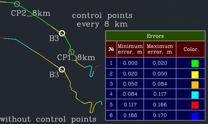
The International Archives of the Photogrammetry, Remote Sensing and Spatial Information Sciences, Volume XLIII-B2-2020, 2020
                                               XXIV ISPRS Congress (2020 edition)

parameters. Angular ones are calculated with IMU which also         many MLS systems. The base-line length between the roving
allows compensating GNSS signal short-term loss in such areas       receiver installed in MLS system and the reference station have
(Altyntsev, Popov, 2014).                                           to be limited to no more than 30 km. If base-line length exceeds
                                                                    this distance a network of reference stations should be used.
GCPs are used to reach absolute accuracy of 5 cm and better         The network must include from 4 to 50 reference stations for
when GNSS signals are poor or they are lost. Schaer and Vallet      processing in POSPac MMS. The maximum distance from the
(2016) demonstrated that GNSS outages longer than 30-60             rover to the nearest reference station in the network is no more
seconds may lead to a rapid decrease in absolute positioning        than about 70 km. To reduce errors the scanning should be
accuracy when driving at 40-50 km/h. In case the GNSS signals       carried out inside a polygon defined by reference stations.
are lost the positional drift reaches its maximum in the middle
of the section. They offered to use GCPs every 400 m to reach a     The final decision about necessity of applying GCPs in
desired accuracy better than 5 cm. To correct MLS trajectory        territories with good GNSS signals or about a choice of average
the manual identification of GCPs in the point cloud is required.   distance between two GCP has to depend on the final
                                                                    production obtained on the basis of an MLS point cloud.
For adjustment of MLS point clouds and trajectories aerial
images can be used. Gao et al. (2015) proposed a framework for      MLS are often applied for mapping of linear long-distance
adjusting MLS point cloud through UAV images automatically.         territories. Topographic plans are created using an MLS point
The main essence of the framework as follows: road marking          cloud. Horizontal and vertical positional accuracy of
extraction from MLS point cloud based on intensity values,          topographic plan’s objects must not exceed values given in SP
interpolation of point cloud intensity data, aerial triangulation   47.13330.2016 «Engineering survey for construction. Basic
of UAV images, pairwise registration of these images and point      principles» (2016). To meet the requirements of this manual
cloud based on feature point extraction with Harris corner          allowable errors are calculated for the certain scale of
keypoint detection, point matching using a local edge-based         topographic plan and contour interval.
template, point cloud adjustment. The accuracy of 6–10 cm was
reached. However, they performed the adjustment of the point        In the paper the method of MLS is analyzed for the goal of
cloud and did not estimate the trajectory accuracy.                 mapping. Next issues are discussed: creating geodetic control
                                                                    network for MLS, the scheme of MLS for long-distance areas,
Hussnain et al. (2018) developed an automatic method of both        adjustment of MLS data including the analysis of accuracy
point cloud and trajectory adjustment in GNSS denied areas by       estimation with different numbers of control points. As
extracting corresponding 3D tie points between aerial images        measuring of control point coordinates with terrestrial classical
and an MLS point cloud. Aerial imagery is an external source of     methods is very time-consuming, it is necessary to determine
GCPs for computing reliable exterior orientation parameters         minimum allowed number of control points for MLS data to
(Hussnain et al., 2019). Using described method they have           match the accuracy of large scale topographic mapping. It
adjusted the MLS trajectory with accuracy of 9–14 cm.               should be also determined the maximum base-line length
                                                                    between the roving receiver of an MLS system and the reference
Javanmardi et al (2017) used multiple reference data sets           station for this goal. The study is carried out on the basis of data
including aerial imagery to adjust MLS point cloud. They            gathered for roads within oil and gas deposits.
developed a sliding window algorithm for matching geometric
features between images and point cloud. As the features a road            2. MAPPING OF OIL AND GAS DEPOSITS
marking was also proposed to apply. Hu et al. (2019) offered to
apply pole-like infrastructures in addition to a road marking for   Oil and gas deposit areas are represented by complicated
trajectory adjustment.                                              industrial infrastructure such as pipelines, buildings, tanks,
                                                                    power lines. A roadway network is constructed among different
Thus, the great number of algorithms and techniques have been       oil and gas areas. For mapping of these areas and roads
developing for poor quality of GNSS measurements in dense           different methods can be used. MLS is preferable for long
urban areas where a lot of GCPs are needed for improving            roads.
accuracy of adjusted MLS data. Measuring of GCP coordinates
with terrestrial classical methods like a tacheometric survey and   In 2017 mobile laser scanning war carried out for a road
a survey using GNSS receivers is very time-consuming. In this       between Talakan oil and gas deposit and Vitim. Vitim is an
case application of aerial imagery can reduce the average           urban locality in Russia. The goal of MLS was creating a
distance between two control points till 100–200 m instead of       topographic plan at a scale of 1:500 with a contour interval of
using hundred control points along the road collected under         0.25 m. The length of the road was 160 km.
field conditions [Gao et al., 2015].
                                                                    The first stage of field works was creating geodetic control
It may be unnecessary to apply GCPs when scanning outside           network for MLS. It was done with Trimble R8 satellite
urban areas in places where GNSS signals are good. Only some        receivers. The scheme of creating geodetic control network is
check points can be applied to be sure of required accuracy.        presented in Figure 1. There were used 6 points of the state
When this occurs application of aerial images becomes               geodetic network for measuring coordinates of 27 geodetic
inefficiently. Classical method will be the best choice. In this    control network points. 4 of 27 points were applied for placing
case we should take into account recommendations about              reference stations while MLS. 24 of 27 points were needed for
maximum base-line length to a reference station. The positional     an employer to carry out additional works connected with road
accuracy gets worse with increasing distance to it. Scherzinger,    maintenance and these points were not used for MLS.
and Hutton (2020), Hutton and Roy (2020) described these
recommendations for data processed in POSPac MMS software
developed by Applanix company. This software helps to adjust
MLS trajectories. Applanix company produces equipment for

                                               This contribution has been peer-reviewed.
                 https://doi.org/10.5194/isprs-archives-XLIII-B2-2020-197-2020 | © Authors 2020. CC BY 4.0 License.                 198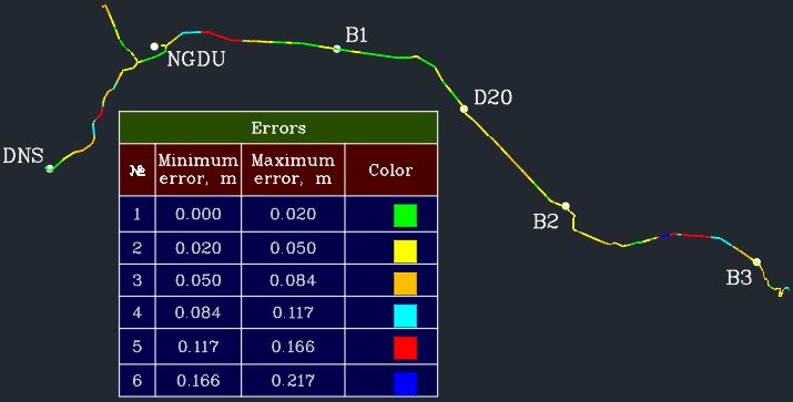
The International Archives of the Photogrammetry, Remote Sensing and Spatial Information Sciences, Volume XLIII-B2-2020, 2020
                                               XXIV ISPRS Congress (2020 edition)

                                                                          3. RELATIVE ADJUSTMENT OF MLS DATA

                                                                    Because of applying only one GNSS receiver each part of the
                                                                    trajectory was adjusted in the POSPac MMS software
                                                                    separately. Adjusted trajectories and raw point cloud data were
                                                                    imported to Riprocess software where coordinates of laser
                                                                    points had been separately calculated for each part of the
                                                                    adjusted trajectory. Automatic adjustment of point cloud’s
                                                                    multi-passes is carried out in Riprocess software accordingly to
  Figure 1. The scheme of creating geodetic control network         an algorithm described by Rieger et al. (2010). The algorithm
                                                                    works well in areas where there are a lot of vertical objects such
The system Riegl VMX-250 was chosen for scanning of the             as walls of buildings. In urban areas horizontal positional errors
road. In this system IMU by Applanix company is applied and         aim for least values even within one part of the trajectory. The
trajectories are processed in POSPac MMS software. According        large errors in horizontal position can occur in areas without
to the requirements described by Hutton and Roy (2020) the          these objects. Vertical positional errors usually aim for least
MLS for this road has to be carried out when at least 4 reference   errors in any type of areas after relative adjustment within one
stations are simultaneously operated. In this case MLS of 160       part of the trajectory.
km could be done in 1 day. The absolute measuring accuracy
for ground point coordinates should have been within 5 cm           Thus, 7 parts of MLS data were separately and automatically
owing to stated specifications of the system.                       adjusted. The adjacent trajectory parts overlapped slightly. To
                                                                    check errors between the adjacent trajectory parts check points
However, it was decided to apply only 1 reference station while     were used. Horizontal and vertical positional errors were
scanning because of safety reasons. The territory is occupied by    estimated independently of each other. To estimate vertical
a large number of wild animals. While MLS each reference            positional errors, check points were automatically found on the
station must operate continuously. To meet this requirement a       road surface in the overlapping areas. To estimate horizontal
surveyor turns on a GNSS receiver on a reference station before     positional errors, check points were manually placed on road
MLS starts and turns off it after MLS finishers. The more           signs. Manual placement of check point was needed because of
reference stations are used the more surveyors are needed.          impossibility for the algorithm to find horizontal positional
Every surveyor must be protected.                                   points. The road Talakan – Vitim was surrounded almost
                                                                    throughout by high vegetation. There were almost no walls
As it was discussed earlier in case of applying only 1 reference    within the surveying territory. In Figure 3 the example of a
station the MLS system shall not be more than 30 km away            manually placed check point is demonstrated.
from it. To provide better accuracy it was decided not to move
more than 15 km away from the station. The territory of
surveying was divided in 7 parts. Laser scanning was carried
out along each part of the territory both in forward and
backward directions with the vehicle’s average speed of 40
km/h. In Figure 2 the scheme of MLS is shown. Geodetic
control network points with numbers of B1, B2, B3 and D20
were used for placing reference stations. NGDU and DNS are
continuously operating reference stations (CORS) that were
used while scanning the western part of the territory. Certain
color of the vehicle’s trajectory demonstrates the reference
station number used for scanning. The trajectory near NGDU
station was divided in 2 parts because MLS of this territory was
conducted for 2 days.

                                                                      Figure 3. Horizontal positional error between point cloud’s
                                                                                             multi-passes

                                                                    The results of the relative accuracy estimation using the check
                                                                    points are given in Table 1. Totally, 56 horizontal check points
                                                                    and 232 vertical ones were used. It is seen that vertical
                                                                    positional maximum error is rather larger in overlapping areas
                                                                    and exceeds stated specifications of the system in several times.
                 Figure 2. The scheme of MLS                                                 X, m           Y, m            Z, m
                                                                         Mean error          0.036          0.046          0.023
At first MLS was conducted for territories within operating the          RMS error           0.040          0.052          0.048
CORS. Then a GNSS receiver mounted on the reference station           Maximum error          0.068          0.084          0.297
with number of B1 operated during MLS of the corresponding           Table 1. Relative accuracy estimation of MLS data using check
trajectory part. After that the receiver was moved to the next                                    points
reference station for scanning the next part of the road. The
territory around the reference station with the number of B3 was    For MLS data adjustment of the whole territory including
scanned in the last turn.                                           overlapping areas half of check points were used as control
                                                                    ones. The remaining check points were applied for accuracy
                                                                    estimation after adjustment. Table 2 illustrates the results of

                                               This contribution has been peer-reviewed.
                 https://doi.org/10.5194/isprs-archives-XLIII-B2-2020-197-2020 | © Authors 2020. CC BY 4.0 License.               199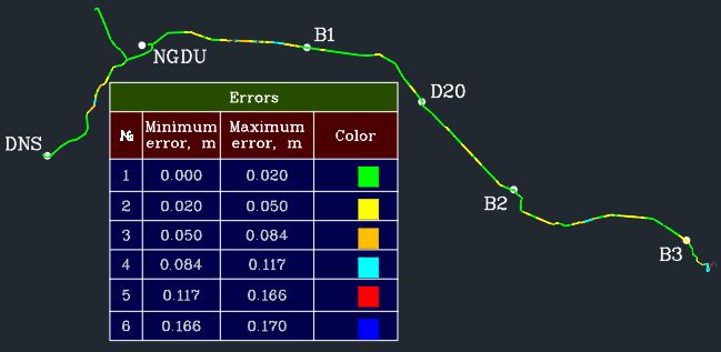
The International Archives of the Photogrammetry, Remote Sensing and Spatial Information Sciences, Volume XLIII-B2-2020, 2020
XXIV ISPRS Congress (2020 edition)
relative accuracy estimation of MLS data adjustment using The final absolute accuracy of MLS data adjustment using
control points, whereas using check points – in Table 3. The control and check point determines the usability of these data
MLS data were adjusted in a UTM projection. for creating topographic plans at a certain scale and a contour
X, m Y, m Z, m interval. According to (Engineering survey for construction.
Mean error 0.009 0.004 0.003 Basic principles., 2016) average errors for horizontal position of
RMS error 0.012 0.007 0.010 objects and terrain contours with clear recognizable edges
Maximum error 0.033 0.025 0.046 should not exceed 0.5 mm at plotting plan scale for not built-up
Table 2. Relative accuracy estimation of MLS data adjustment areas relative to the nearest points of a geodetic control
using control points network. Average errors for their vertical position should not
exceed 1/4 of the accepted contour interval for flat terrain
X, m Y, m Z, m (surface slope up to 2º) and 1/3 – for surface slope greater than
Mean error 0.013 0.011 0.007 2º. Maximum errors shall not exceed twice values of mean
RMS error 0.020 0.013 0.016 errors in both horizontal and vertical positions. Errors
Maximum error 0.037 0.036 0.055 exceeding the maximum allowed values should be eliminated.
At the same time the number of them shall not exceed 10% of
Table 3. Relative accuracy estimation of MLS data adjustment
the total number of check measurements.
using check points
The average slope of the surveyed road was greater than 2º. For
4. ABSOLUTE ADJUSTMENT OF MLS DATA
the scale of 1:500 horizontal positional accuracy must not
Topographic plan at a scale of 1:500 must have been created in exceed 25 cm for mean values and 50 cm for maximum ones.
a local coordinate system required for the employer. To For the contour interval of 25 cm vertical one must not exceed
transform MLS data from UTM coordinates to local ones 8 8.3 cm for mean values and 16.6 cm for maximum ones.
points of the geodetic network showed in Figure 1 were used:
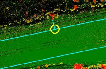
B1, B2, B3, D20, REPER 782, DNS, NGDU and Viski. These Based on calculated tolerances and the fact that the quality of
points were evenly distributed within the surveying area. Local GNSS measurements for the road Talakan – Vitim was well, the
coordinates of these points were known and UTM coordinates quantity of required ground control points had to be not so large
were measured with GNSS receivers. At first, there were comparing to urban areas. It was decided to place ground points
calculated transformation parameters using 3D affine along the road every 1 km. In Figure 4 the example of placing
transformation with 9 parameters which is defined by equations ground points is shown. They were located on the road surface
(Wu et al., 2013): edge in opposite of distance marks. It is the center of yellow
circle. A distance mark is shown in the form of red symbol.
Parallel cyan lines display road edges. GNSS receivers were
X A x0 XB used for measuring coordinates of ground points. The maximum
Y = y + S (λ ) S (λ ) S (λ ) × R (ω ) R (ϕ ) R (κ ) Y (1)
A 0 1 2 3 B error of measuring ground point coordinates did not exceed 3
Z A z0 Z B cm relatively to geodetic control network in horizontal and
vertical position.
where XA, YA, ZA = local coordinates
XB, YB, ZB = UTM coordinates
x0, y0, z0 = the translation parameters of origin of the two
coordinate systems
λ1, λ2, λ3 = the scale parameter of the two coordinate
systems
ω, φ, κ = the rotation angles of the two coordinate
systems
Table 4 demonstrates the accuracy of transforming 8 geodetic
network points from UTM coordinates to local ones using Figure 4. The example of placing ground points
calculated 3D affine transformation parameters. The calculated
3D affine transformation parameters were applied for Ground point locations were identified in the point cloud. At
transforming MLS data from UTM projection to the local first ground points were used as check ones. There were
coordinate system. calculated distances between ground points measured in the
X, m Y, m Z, m point cloud and those measured with GNSS receivers. The
Mean error 0.001 0.001 0.030 results of calculations are given in Table 5.
RMS error 0.001 0.001 0.034 X, m Y, m Z, m
Maximum error 0.001 0.001 0.06 Mean error 0.009 0.010 0.047
Table 4. Accuracy estimation of transforming geodetic network RMS error 0.016 0.022 0.041
point coordinates Maximum error 0.116 0.228 0.218
Table 5. Absolute accuracy estimation of MLS data adjustment
To estimate accuracy of transformed MLS data it is necessary to using check points every 1 km and without control points
use control and check points placed within the point cloud
which coordinates are measured with more accurate land It is seen from the Table 5 that horizontal positional accuracy is
surveying equipment such as GNSS receivers and total stations. appropriate for creating topographic plans at a scale of 1:500,
whereas vertical one is too large. The value of maximum error
exceeds the calculated tolerance. It means that application of
control points for adjustment is necessary. A trajectory part with
This contribution has been peer-reviewed.
https://doi.org/10.5194/isprs-archives-XLIII-B2-2020-197-2020 | © Authors 2020. CC BY 4.0 License. 200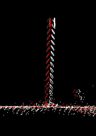
The International Archives of the Photogrammetry, Remote Sensing and Spatial Information Sciences, Volume XLIII-B2-2020, 2020
                                               XXIV ISPRS Congress (2020 edition)

the maximum error is seen from Figure 5 which demonstrates
error distribution. It is the place in the middle of the trajectory
part between control network points with numbers of B2 and
B3. A direct distance between these network points is 29 km.
The trajectory part with errors exceeding the calculated
tolerance of 16.6 cm for vertical measurements is located at a
distance of 14.5 km from B2 and 13.4 km from B3. It can be
assumed that placing 1 control point in the middle of this
trajectory part would be sufficient to meet the tolerance. Error
distribution for other trajectory parts does not exceed the              Figure 6. Error distribution for MLS data adjustment using
tolerance. The length of the other trajectory parts is less than the       check points every 2 km and control points every 2 km
one between B2 and B3. It is 23.5 km between DNS and
NGDU, 26.7 km between NGDU and B1, 20.5 km between B1                  Next, it was decided to take every fourth ground point as
and D20, 20.5 km between D20 and B2.                                   control one, the others – as check ones. The results of accuracy
                                                                       estimation with this number of control and check points are
                                                                       given in Table 7. Figure 7 demonstrates error distribution for
                                                                       MLS data adjustment using check points every 1 km and
                                                                       control points every 4 km. Comparing to the previous results
                                                                       the values of errors were not dramatically changed.
                                                                                                X, m           Y, m           Z, m
                                                                            Mean error          0.014         0.013          0.020
                                                                            RMS error           0.020         0.017          0.023
                                                                          Maximum error         0.123         0.098          0.117
                                                                        Table 7. Absolute accuracy estimation of MLS data adjustment
                                                                         using check points every 1 km and control points every 4 km
  Figure 5. Error distribution for MLS data using check points
             every 1 km and without control points

To obtain adjusted point cloud with high accuracy and within
the tolerance it was decided to study how point cloud
adjustment results depend on the number of control points and
distances between them. In case of applying all ground points as
control ones, errors from the Table 5 equal to zero. It is due to
the algorithm used for transformation of the MLS data. The
algorithm is optimized for local accuracy. It means that this
algorithm transforms the source point cloud exactly to target            Figure 7. Error distribution for MLS data adjustment using
control points. Transformation is carried out with specifying              check points every 1 km and control points every 4 km
difference values in every control point for northing, easting
and elevation.                                                         At the end every eighth ground point was taken as control one,
                                                                       the others – as check ones. Table 8 shows accuracy estimation
Without check points absolute accuracy estimation does not             results of MLS data adjustment with such number of check
seem complete. For this reason, ground points were divided             points and Figure 8 – error distribution.
equally into control and check ones. In other words, both check                                 X, m            Y, m         Z, m
and control points were used every 2 km. Absolute accuracy                  Mean error          0.018          0.016         0.028
estimation of MLS data adjustment using control and check                   RMS error           0.028          0.020         0.033
points every 2 km is given in Table 6.                                    Maximum error         0.170          0.110         0.170
                         X, m          Y, m           Z, m              Table 8. Absolute accuracy estimation of MLS data adjustment
     Mean error         0.014          0.017          0.020              using check points every 1 km and control points every 8 km
     RMS error          0.016          0.016          0.022
   Maximum error        0.085          0.064          0.110
 Table 6. Absolute accuracy estimation of MLS data adjustment
  using check points every 2 km and control points every 2 km

Maximum error of vertical position was decreased in 2 times
and started to be within the tolerance. This means that
application of control points every 2 km is enough for scanning
this road. Figure 6 demonstrates error distribution for MLS data
adjustment using check points every 2 km and control points
every 2 km. The trajectory part with the maximum error is
located between control network points with numbers of B2 and
B3 as for MLS data adjusted without control points.                      Figure 8. Error distribution for MLS data adjustment using
                                                                           check points every 1 km and control points every 8 km

                                                                       Table 8 demonstrates that the maximum error exceeds the
                                                                       calculated tolerance and Figure 8 shows the part of the

                                                This contribution has been peer-reviewed.
                  https://doi.org/10.5194/isprs-archives-XLIII-B2-2020-197-2020 | © Authors 2020. CC BY 4.0 License.               201
The International Archives of the Photogrammetry, Remote Sensing and Spatial Information Sciences, Volume XLIII-B2-2020, 2020
XXIV ISPRS Congress (2020 edition)
trajectory with this error. The place with the maximum error is are almost no vertical walls horizontal positional errors will be
located at the start of the road near the control network point much greater than for urban areas. Additional manual
with the number of B3. The accuracy of MLS data adjustment adjustment is needed. For roads distance marks can be used as
became worse in this trajectory part. The comparison of the horizontal control points.
trajectory obtained without adjustment using control points and
the one obtained with control points every 8 km is shown in The results of absolute accuracy estimation demonstrate that not
Figure 9. It can be explained by the fact that a control point so many control points are required to adjust MLS data if the
with the number CP1 is located rather far from the start of the goal of laser scanning is large scale topographic mapping of
road (4 km in direct direction). long-distance areas with open view of the sky. For the Riegl
VMX-250 system it is enough to measure coordinates of control
points every 8 km. Control points should be placed on the road
surface. They also must be located at the very beginning and the
end of a trajectory.
In spite of recommendation of Scherzinger and Hutton (2020),
Hutton and Roy (2020), the results of the study also showed
that for creating topographic plans at a scale of 1:500 with a
contour interval of 0.25 cm it is not recommended to increase
the base-line length between the roving receiver installed in
MLS system and the reference station by more than 13 km to
have the opportunity not to use control points on the road. In
the contrary case ground-based surveying methods should be
Figure 9. The comparison of the trajectoriy adjusted with used for absolute adjustment of MLS data. Aerial methods are
control points every 8km and the trajectory without adjustment not efficient to use as a source of control points even if the
using control points GNSS signal is continuous and has good quality.
To eliminate large errors at the start of the road it should be REFERENCES
have used a control point with the number of CP0 showed in
Figure 10 instead of the one with the number of CP1. The Altyntsev, M. A., Popov R.A., 2014. The Analysis of GPS
ground point CP0 was used as control one when using control Signal Short-term Loss Influence on the Accuracy of Mobile
points every 2 km. Laser Scanning Data. XXV FIG Congress, 16-21 June 2014,
Malaysia, Kuala Lumpur.
Ding, W., Wang, J., Rizos, C., Kinlyside, D., 2007. Improving
adaptive Kalman estimation in GPS/INS integration. Journal of
Navigation, 60(03), 517–529.
doi.org/10.1017/S0373463307004316
Gao, Y., Huang, X., Zhang, F., Fu, Z., Yang, C., 2015.
Automatic geo-referencing mobile laser scanning data to UAV
images. ISPRS – International Archives of the Photogrammetry,
Remote Sensing and Spatial Information Sciences, XL-1/W4,
Figure 10. The choice of placing control points 41–46. doi.org/10.5194/isprsarchives-XL-1-W4-41-2015.
No further increase in distance between control points is Guan, H., Li, J., Yu, Y., Wang, C., Chapman, M., Yang, B.,
required because of limited distance between reference station. 2014. Using mobile laser scanning data for automated
Thus, it may be concluded that for the goal of large scale extraction of road markings. ISPRS Journal of Photogrammetry
topographic mapping application of control points every 8 km is and Remote Sensing. 87 (2014), 93–107.
enough for scanning a road outside urban areas with Riegl
VMX-250 system when a GNSS signal is good. In this case it Hu., H., Sons., M., Stiller. C., 2019. Accurate Global Trajectory
must be provided measuring control points at the very edges of Alignment using Poles and Road Markings.
trajectories. arXiv:1903.10205v1.
Application of fewer amount of control points allows to speed Hussnain, Z., Oude Elbernk, S., Vosselman., G., 2018. An
up the process of field surveying works. If a distance between automatic procedure for mobile laser scanning platform 6dof
nearest reference stations does not exceed 26.7 km, as the trajectory adjustment. ISPRS – International Archives of the
distance between control network points NGDU and B1, and Photogrammetry, Remote Sensing and Spatial Information
GNSS conditions are excellent control points may not be Sciences, XLII-1, 203–209. doi.org/10.5194/isprs-archives-
required. In this case half of the distance should be scanned XLII-1-203-2018.
when launching one reference station, and the second half –
Hussnain, Z., Oude Elbernk, S., Vosselman., G., 2019.
when launching a nearby station.
Automatic extraction of accurate 3D tie points for trajectory
adjustment of mobile laser scanners using aerial imagery. ISPRS
5. CONCLUSION
Journal of Photogrammetry and Remote Sensing, 154, 41–58.
The results of relative accuracy estimation of data adjusted with doi.org/10.1016/j.isprsjprs.2019.05.010.
automatic algorithms shows that if around surveying area there
This contribution has been peer-reviewed.
https://doi.org/10.5194/isprs-archives-XLIII-B2-2020-197-2020 | © Authors 2020. CC BY 4.0 License. 202The International Archives of the Photogrammetry, Remote Sensing and Spatial Information Sciences, Volume XLIII-B2-2020, 2020
XXIV ISPRS Congress (2020 edition)
Javanmardi, M., Javanmardi, E., Gu, Y., Kamijo, S., 2017.
Automatic calibration of 3D mobile laser scanning using aerial
surveillance data for precise urban mapping. IEEE Intelligent
Vehicles Symposium (IV), Los Angeles, CA, 1182–1188.
doi.org/10.1016/j.isprsjprs.2019.05.010.
Julge, K., Vajakas, T., Ellmann, A., 2017. Performance analysis
of a compact and low-cost mapping-grade mobile laser scanning
system. Journal of Applied Remote Sensing, 11(4), 044003.
Levinson, J., Montemerlo, M., Thrun, S., 2007. Map-Based
Precision Vehicle Localization in Urban Environments.
Robotics: Science and Systems III.
doi.org/10.15607/RSS.2007.III.016
Rieger, P., Studnicka, N., Pfennigbauer, M., 2010. Boresight
alignment method for mobile laser scanning systems. Journal of
Applied Geodesy, 4(1), 13–21. doi.org/10.1515/JAG.2010.002.
Schaer, P., Vallet, J., 2016. Trajectory adjustment of mobile
laser scan data in GPS denied environments. ISPRS –
International Archives of the Photogrammetry, Remote Sensing
and Spatial Information Sciences, XL-3/W4, 61–64.
doi.org/10.5194/isprsarchives-XL-3-W4-61-2016.
Wang., Y., Chen., Q., Zhu., Q., Liu., L., Li., C., Zheng., D.,
2019. A Survey of Mobile Laser Scanning Applications and
Key Techniques over Urban Areas. Remote Sensing, 11(13),
1540. doi.org/10.3390/rs11131540.
Wu, C.-T., Hsiao, C.-Y., Chen, C.-S., 2013. Improvement of
LiDAR data accuracy using 12 parameter affine transformation.
Journal of Chinese Soil and Water Conservation, 44(4), 293–
301.
Zhao, Y., 2011. GPS/IMU integrated system for land vehicle
navigation based on MEMS. KTH Royal Institute of
Technology, 85.
SP 47.13330.2016 «Engineering survey for construction. Basic
principles», 2016, Moscow, TSNIIGAiK (in Russian).
Hutton, J., Roy, E. The Applanix SmartBase software for
improved robustness, accuracy, and productivity of mobile
mapping and positioning
https://www.applanix.com/pdf/applanix%20smartbase.pdf, (12
January 2020).
Scherzinger, B., Hutton, J. Applanix In-Fusion technology
explained https://www.applanix.com/pdf/Applanix_IN-
Fusion.pdf (12 January 2020).
This contribution has been peer-reviewed.
https://doi.org/10.5194/isprs-archives-XLIII-B2-2020-197-2020 | © Authors 2020. CC BY 4.0 License. 203You can also read